Execution time varied by applications, input size, and the number of en- ...... proposes a compiler/runtime framework th
VIRTUALIZING DATA PARALLEL SYSTEMS FOR PORTABILITY, PRODUCTIVITY, AND PERFORMANCE
by Janghaeng Lee
A dissertation submitted in partial fulfillment of the requirements for the degree of Doctor of Philosophy (Computer Science and Engineering) in the University of Michigan 2015
Doctoral Committee: Professor Scott Mahlke, Chair Nathan Clark, Virtu Financial Associate Professor Kevin Pipe Assistant Professor Lingjia Tang Associate Professor Thomas Wenisch
c
Janghaeng Lee
2015
All Rights Reserved
To my family
ii
ACKNOWLEDGEMENTS
I would like to express my first and foremost gratitude to my research advisor, Professor Scott Mahlke, for his continuous support of this research. I consider myself truly lucky to have worked with him these past years. He has shown incredible patience, served as an excellent mentor from immense knowledges, encouraged me all the time, and guided pathways to success in this field. My sincere gratitude also goes to my thesis committee, Prof. Thomas Wenisch, Prof. Kevin Pipe, Prof. Lingia Tang, and Nathan Clark for providing excellent comments and suggestions that helped me to make this work more valuable. I am grateful to Nathan Clark, the former advisor at Georgia Tech, who brought me to this area and enlightened me the first sight of research in this field. Also, I thank to Neungsoo Park who led me out into the graduate study in the United States. It was very fortunate to be a member of Compilers Creating Custom Processors (CCCP) research group. I specially thank to Mehrzad Samadi, who is a great collaborator throughout years, providing significant helps in this work. It would not possible to have my thesis in the current shape without his support. I would also like thank a number of other students and alumni in the CCCP research group: Shantanu Gupta, Yongjun Park, Hyoun Kyu Cho, Ankit Sethia, Gaurav Chadha, Anoushe Jamshidi, Daya Khudia, Andrew Lukefahr, Shruti
iii
Padmanabha, Jason Jong Kyu Park, John Kloosterman, Babak Zamirai, and Jiecao Yu. All the people in the group are tightly bound together helping each other, and they made my PhD life much more enjoyable. In particular, Mehrzad, Ankit and Daya gave funnyand-stupid jokes all the time although I do not care, Jason Jong Kyu helped me when I encountered with math problems, and Shantanu played a great role as a mentor during my internship at Intel, giving me an opportunity to work on a great project. My special thanks are extended to my Korean friends who made my time in Ann Arbor more enjoyable. Especially, I thank to Jason Jong Kyu Park and Eugene Kim as I could have tasty meals every dinner. Finally and most importantly, my family deserves endless gratitude. My father, Jungsik Lee, and my mother, Sunmee Kim, always gave me the unconditional love and support. Whatever I am, I stand here because of them. I appreciate my brothers, Jihaeng and Jangwook. I have unforgettable childhood memories with them. They are always supportive and encouraging all the time.
iv
TABLE OF CONTENTS
DEDICATION . . . . . . . . . . . . . . . . . . . . . . . . . . . . . . . . . . .
ii
ACKNOWLEDGEMENTS . . . . . . . . . . . . . . . . . . . . . . . . . . . .
iii
LIST OF FIGURES . . . . . . . . . . . . . . . . . . . . . . . . . . . . . . . .
viii
LIST OF TABLES . . . . . . . . . . . . . . . . . . . . . . . . . . . . . . . . .
xii
ABSTRACT . . . . . . . . . . . . . . . . . . . . . . . . . . . . . . . . . . . . .
xiii
CHAPTER I. Introduction . . . . . . . . . . . . . . . . . . . . . . . . . . . . . . . . . 1.1 1.2
Challenges of Using Multiple GPUs Contributions . . . . . . . . . . . . 1.2.1 SKMD . . . . . . . . . . 1.2.2 VAST . . . . . . . . . . . 1.2.3 MKMD . . . . . . . . . .
. . . . .
. . . . .
. . . . .
. . . . .
. . . . .
. . . . .
. . . . .
. . . . .
. . . . .
. . . . .
. . . . .
. . . . .
. . . . .
. . . . .
. . . . .
1
. . . . .
3 5 5 6 7
II. Background . . . . . . . . . . . . . . . . . . . . . . . . . . . . . . . . .
9
III. SKMD: Single Kernel Execution on Multiple Devices . . . . . . . . . . 12 3.1 3.2
3.3
Introduction . . . . . . . . . . . . . . . . . . . . . . . . . . . . SKMD System . . . . . . . . . . . . . . . . . . . . . . . . . . . 3.2.1 Kernel Transformation . . . . . . . . . . . . . . . . . 3.2.2 Buffer Management . . . . . . . . . . . . . . . . . . 3.2.3 Performance Prediction . . . . . . . . . . . . . . . . . 3.2.4 Transfer Cost and Performance Variation-Aware Partitioning . . . . . . . . . . . . . . . . . . . . . . . . . 3.2.5 Limitations . . . . . . . . . . . . . . . . . . . . . . . Evaluation . . . . . . . . . . . . . . . . . . . . . . . . . . . . . v
. . . . .
12 17 19 25 26
. 29 . 35 . 36
3.4 3.5
3.3.1 Results and Analysis . . . . . . . 3.3.2 Execution Time Break Down . . . 3.3.3 Performance Prediction Accuracy Related Work . . . . . . . . . . . . . . . . Conclusion . . . . . . . . . . . . . . . . . .
. . . . .
. . . . .
. . . . .
. . . . .
. . . . .
. . . . .
. . . . .
. . . . .
. . . . .
. . . . .
. . . . .
. . . . .
40 43 46 48 51
IV. VAST: Virtualizing Address Space for Throughput Processors . . . . . 52 4.1 4.2 4.3
4.4
4.5
4.6
4.7 4.8
Introduction . . . . . . . . . . . . . . . . . . Motivation . . . . . . . . . . . . . . . . . . . VAST System Overview . . . . . . . . . . . . 4.3.1 VAST System Execution Flow . . . 4.3.2 VAST Execution Timeline . . . . . Implementation . . . . . . . . . . . . . . . . 4.4.1 The Design of Page Accessed Set . 4.4.2 OpenCL Kernel Transformation . . 4.4.3 Look-ahead Page Table Generation 4.4.4 Forwarding Shared Pages . . . . . . Further Optimization . . . . . . . . . . . . . 4.5.1 Selective Transfer . . . . . . . . . . 4.5.2 Zero Copy Memory . . . . . . . . . 4.5.3 Double Buffering . . . . . . . . . . Evaluation . . . . . . . . . . . . . . . . . . . 4.6.1 Results . . . . . . . . . . . . . . . 4.6.2 Page Lookup Overhead . . . . . . . Related Work . . . . . . . . . . . . . . . . . Conclusion . . . . . . . . . . . . . . . . . . .
. . . . . . . . . . . . . . . . . . .
. . . . . . . . . . . . . . . . . . .
. . . . . . . . . . . . . . . . . . .
. . . . . . . . . . . . . . . . . . .
. . . . . . . . . . . . . . . . . . .
. . . . . . . . . . . . . . . . . . .
. . . . . . . . . . . . . . . . . . .
. . . . . . . . . . . . . . . . . . .
. . . . . . . . . . . . . . . . . . .
. . . . . . . . . . . . . . . . . . .
. . . . . . . . . . . . . . . . . . .
52 56 57 58 60 61 61 63 67 69 71 71 73 74 74 77 81 83 86
V. MKMD: Multiple Kernel Execution on Multiple Devices . . . . . . . . 88 5.1 5.2 5.3 5.4
5.5
5.6 5.7
Introduction . . . . . . . . . . . . . . . . . . MKMD Overview . . . . . . . . . . . . . . . Execution Time Modeling . . . . . . . . . . . MKMD Scheduling . . . . . . . . . . . . . . 5.4.1 Kernel Graph Construction . . . . . 5.4.2 Coarse-grain Scheduling . . . . . . 5.4.3 Fine-grain Multi-kernel Partitioning 5.4.4 Partitioning a Kernel to Time Slots . 5.4.5 Overhead and Limitations . . . . . Evaluation . . . . . . . . . . . . . . . . . . . 5.5.1 Results . . . . . . . . . . . . . . . 5.5.2 Sensitivity to Profiles . . . . . . . . 5.5.3 Case Study . . . . . . . . . . . . . RELATED WORK . . . . . . . . . . . . . . Conclusion . . . . . . . . . . . . . . . . . . . vi
. . . . . . . . . . . . . . .
. . . . . . . . . . . . . . .
. . . . . . . . . . . . . . .
. . . . . . . . . . . . . . .
. . . . . . . . . . . . . . .
. . . . . . . . . . . . . . .
. . . . . . . . . . . . . . .
. . . . . . . . . . . . . . .
. . . . . . . . . . . . . . .
. . . . . . . . . . . . . . .
. . . . . . . . . . . . . . .
88 91 93 99 99 100 102 105 109 110 112 114 117 118 120
VI. Conclusion . . . . . . . . . . . . . . . . . . . . . . . . . . . . . . . . . . 122 6.1 6.2
Summary . . . . . . . . . . . . . . . . . . . . . . . . . . . . . . . 122 Future Directions . . . . . . . . . . . . . . . . . . . . . . . . . . 124
BIBLIOGRAPHY . . . . . . . . . . . . . . . . . . . . . . . . . . . . . . . . . 126
vii
LIST OF FIGURES
Figure 1.1
3.1 3.2 3.3 3.4 3.5 3.6
3.7
3.8
3.9 3.10
3.11
Challenges in exploiting multiple GPUs for large data sets. Because the programming model exposes the hardware details, programmers must consider portability, productivity, and performance when they write the data parallel kernels with large data on multiple devices. . . . . . . . . Physical OpenCL computing devices with different performances, memory spaces, and bandwidths. . . . . . . . . . . . . . . . . . . . . . . . The SKMD framework consisting of four units: Kernel Transformer, Buffer Manager, Partitioner, and Profile Database. . . . . . . . . . . . OpenCL’s N-Dimensional range . . . . . . . . . . . . . . . . . . . . . Partition-ready Blackscholes kernel. . . . . . . . . . . . . . . . . . . . Different memory access patterns of kernels . . . . . . . . . . . . . . . Merge Kernel Transformation Process. Only global output parameters, call and put in (a), are marked for merging. Using data flow analysis, store values to global output parameters are replaced with GPU’s partial results, and then proceed with dead code elimination (b). As a result, the merge kernel does not have computational part (c). . . . . . . . . . . . Execution time varied by applications, input size, and the number of enabled work-groups. Depending on the application and input size, the number of enabled work-groups impacts on the execution time differently. . . . . . . . . . . . . . . . . . . . . . . . . . . . . . . . . . . . Performance impact on VectorAdd varying the number of work-groups. The execution time of GPUs do not scale down in spite of reduced number of work-groups. . . . . . . . . . . . . . . . . . . . . . . . . . . . . . . Comparison of linear partitioning and ideal partitioning . . . . . . . . . Speedup and work-group distribution. Each benchmark has different baseline (a), as the fastest device differ by kernels. The fastest device is determined with regard to the execution time and data transfer cost. . Break down of the execution time on each device. The bars on the top is the baseline, which is the fastest single-device execution. SKMD considers the transfer cost, and offloads work-groups in order to balance the workload among the three devices. . . . . . . . . . . . . . . . . . . . .
viii
.
2
. 14 . . . .
16 18 20 21
. 22
. 27
. 29 . 31
. 41
. 44
3.12
4.1
4.2
4.3
4.4
4.5
4.6 4.7
4.8
4.9
Performance prediction accuracy. L2-Norm error (a) shows Euclidean distance between the real execution time and the predicted execution time in milliseconds. Average error rate (b) shows the average percentage of errors in predictions. . . . . . . . . . . . . . . . . . . . . . . . . . . . The code transformation for partial execution of an OpenCL kernel. The kernel takes two additional arguments for the work-group range to execute, and grey backgrounded code is also inserted at the beginning of the kernel to check if the work-group is to be executed. The work-groups out of the range will terminate the execution immediately. . . . . . . . . . The VAST system located between applications and OpenCL library. VAST takes an OpenCL kernel and transforms it into the inspector kernel and the paged access kernel. At kernel launch, the GPU generates PASs (P ASgen) by launching the inspector kernel, then transfers them to the host to create LPT and frame buffer (LP T gen). Next, LPT and frame buffer are transferred to the GPU in order to execute the paged access kernel. . . . . . . . . . . . . . . . . . . . . . . . . . . . . . . . . . . Execution timeline for VAST system. Only PAS generation and the first LPT generation cost is exposed. Other LPT generations and array recoveries are overlapped from data transfer and kernel execution. With double buffering, the second LPT generation starts immediately after the first LPT generation. . . . . . . . . . . . . . . . . . . . . . . . . . . . The design of Page Accessed Set (PAS). Each work-group has its own PAS for each global argument. Each entry of PAS has a boolean value that represents whether corresponding page has been accessed by the workgroup. . . . . . . . . . . . . . . . . . . . . . . . . . . . . . . . . . . . Data flow graphs for the kernel transformation. In the inspector kernel (a), all computational code are removed by dead code elimination. In paged access kernel (b), the base and the offset are replaced with new nodes for address translation. . . . . . . . . . . . . . . . . . . . . . . . The design of Look-ahead Page Table (LPT) and frame buffer. One pair of LPT and frame buffer corresponds to one global argument. . . . . . PAS generation for shared pages (shared PAS). Each reduced PAS is used for a single sequence of partial execution. As the sequence of partial execution increases, the number of logical operations increase for shared PAS as VAST should check pages used in the previous sequences. . . . Execution timeline after optimizations. Selective input transfer removes the cost of frame generation (a). Zero copy memory for output buffer removes the cost of array recovery (b). Double buffering overlaps the input transfer with kernel executioans (c). . . . . . . . . . . . . . . . . Benchmark specifications. For the speedup over the CPU-baseline, data size more than GPU memory is used (a). For the comparison with normal GPU execution, data size less than GPU memory is used (b). . . . . . .
ix
. 47
. 56
. 58
. 60
. 62
. 64 . 65
. 69
. 72
. 77
4.10
4.11
4.12
4.13
5.1
5.2
5.3 5.4
5.5
5.6
5.7
5.8 5.9
Speedup of VAST over Intel OpenCL execution with 4 KB page frame size. VAST does selective transfers for input buffers. VAST+ZC uses selective transfers for input buffers and zero copy memory for output buffers. VAST+ZCDB uses all optimization techniques discussed in Section 4.5. . . . . . . . . . . . . . . . . . . . . . . . . . . . . . . . . . . Speedup of VAST over the GPU-baseline. The performance was measured using small workloads that fits into GPU memory. GPU-ZC is the execution using zero copy memory for all buffers. . . . . . . . . . . . Paged access kernel execution time normalized to the original kernel execution time. Working set size for each benchmark is less than 2 GB. Paged-access kernel execution does not use zero copy memory. . . . . Performance counters collected on N-body with 256K particles. Pagedaccess kernel has approximately 60 million more instructions (a), and 20 million more load transactions for page lookups (b). However, Pagedaccess kernel experiences higher IPC (f), because it gets more L2 hit rate (i). . . . . . . . . . . . . . . . . . . . . . . . . . . . . . . . . . . . . A kernel graph for solving a matrix equation, A2 BB T CB, consisting of six kernels. The system is equipped with different computing devices with separated physical memory. Devices are connected through PCI express (PCIe) interconnect. Each kernel has different amount of computation, and each device has different performance. . . . . . . . . . . . . MKMD workflow that operates in profiling mode and execution mode. In profiling mode, MKMD builds a mathematical model with a set of profile data for the execution time prediction. In execution mode, MKMD predicts the execution time of kernels on various input sizes using the model, and schedules kernels based on the predicted time. . . . . . . . Upper bounds of trip count. The upper bounds are statically determined for (b) . . . . . . . . . . . . . . . . . . . . . . . . as N for (a), and N T Scalability of execution time on NVIDIA GTX760 varying input sizes and the number of enabled work-items (T ). The execution time is linear to the value of cost function T f (x1 , ..., xN ). . . . . . . . . . . . . . . . Coarse-grain scheduling result on three heterogeneous devices. Dotted arrows presents the buffer transfer between devices. PCI bus operates in full-duplex, but GTX760 and i3770 experience input and output congestion respectively. . . . . . . . . . . . . . . . . . . . . . . . . . . . . . Available compute-time slots (dotted-squares) for partitioning kernel 3. Because kernel 3 depends on kernel 2 (arrow), the lower bound and upper bound of available time slots are the finish time of kernel 2 and 3 respectively. . . . . . . . . . . . . . . . . . . . . . . . . . . . . . . . . Kernel partitioning process. The decimal numbers in a parenthesis shows the ratio of work-groups. The mark (M) is the cost for mering nonlinear outputs. . . . . . . . . . . . . . . . . . . . . . . . . . . . . . . . . . . (a) Speedup of MKMD over in-order executions, and (b) the average device idle time normalized to the finish time. . . . . . . . . . . . . . . . MKMD scheduling overhead. . . . . . . . . . . . . . . . . . . . . . . x
. 78
. 79
. 81
. 84
. 89
. 92 . 95
. 96
. 101
. 103
. 108 . 112 . 113
5.10
5.11
5.12 5.13
Error rates and L2-norm error in milliseconds varying the number of profiles for the execution time modeling. CPU has relatively high error rates on memory-intensive kernels as shown in (a), (b), and (c), but the execution time of these kernels is trivial as they do not have much computation. As a result, the absolute error (L2-norm) in time is also small as illustrated in (d), (e), (f), and (g). . . . . . . . . . . . . . . . . . . . . . . . . . . MKMD total execution time with different timing models varying the number of profiles. The baseline is the execution time scheduled with the model from 80 profiles. This result shows that the entire scheduling time is not sensitive to the number of profiles. . . . . . . . . . . . . . . . . Kernel graph for triple commutator. . . . . . . . . . . . . . . . . . . . Execution timeline for triple commutator. Because matrix computation is too expensive on i3770, (a) the coarse-grain scheduler does not schedule any matrix multiplication kernel on it while GPUs take more than 4 kernels. With MKMD, (b) all devices are almost fully utilized. . . . . .
xi
. 115
. 116 . 117
. 118
LIST OF TABLES
Table 3.1 3.2
3.3
4.1 5.1
5.2 5.3
Experimental setup. . . . . . . . . . . . . . . . . . . . . . . . . . . . . Benchmark specification. VectorAdd, Blackscholes, BinomialOption, and ScanLargeArrays are classified as contiguous kernels, whereas others are defined as discontiguous kernels. . . . . . . . . . . . . . . . . . . . . . . Profile execution parameters and real execution parameters for evaluating performance prediction accuracy. For each profile, 16 profile data was collected varying the number of work-groups. . . . . . . . . . . . . . . . Experimental Setup . . . . . . . . . . . . . . . . . . . . . . . . . . . . . Execution time estimation on NVIDIA GTX 760. The cost functions, f (x1 , ..., xN ), were statically analyzed. For example, 8th Arg means that the value of the 8th argument is the trip count of a loop in the kernel. LocalSize(0) means the work-item count per work-group in the first dimension, while the constant 1 means that a loop was not found in the kernel. . . . . . . . . . . . . . . . . . . . . . . . . . . . . . . . . . . . Experimental Setup . . . . . . . . . . . . . . . . . . . . . . . . . . . . . Benchmark Specification . . . . . . . . . . . . . . . . . . . . . . . . . .
xii
36
38
46 75
98 110 111
ABSTRACT
VIRTUALIZING DATA PARALLEL SYSTEMS FOR PORTABILITY, PRODUCTIVITY, AND PERFORMANCE by Janghaeng Lee
Chair: Scott Mahlke
Computer systems equipped with graphics processing units (GPUs) have become increasingly common over the last decade. In order to utilize the highly data parallel architecture of GPUs for general purpose applications, new programming models such as OpenCL and CUDA were introduced, showing that data parallel kernels on GPUs can achieve speedups by several orders of magnitude. With this success, applications from a variety of domains have been converted to use several complicated OpenCL/CUDA data parallel kernels to benefit from data parallel systems. Simultaneously, the software industry has experienced a massive growth in the amount of data to process, demanding more powerful workhorses for data parallel computation. Consequently, additional parallel computing devices such as extra GPUs and co-processors are attached to the system, expecting more performance and capability to process larger data. However, these programming models expose hardware details to programmers, such as xiii
the number of computing devices, interconnects, and physical memory size of each device. This degrades productivity in the software development process as programmers must manually split the workload with regard to hardware characteristics. This process is tedious and prone to errors, and most importantly, it is hard to maximize the performance at compile time as programmers do not know the runtime behaviors that can affect the performance such as input size and device availability. Therefore, applications lack portability as they may fail to run due to limited physical memory or experience suboptimal performance across different systems. To cope with these challenges, this thesis proposes a dynamic compiler framework that provides the OpenCL applications with an abstraction layer for physical devices. This abstraction layer virtualizes physical devices and memory sub-systems, and transparently orchestrates the execution of multiple data parallel kernels on multiple computing devices. The framework significantly improves productivity as it provides hardware portability, allowing programmers to write an OpenCL program without being concerned of the target devices. Our framework also maximizes performance by balancing the data parallel workload considering factors like kernel dependencies, device performance variation on workloads of different sizes, the data transfer cost over the interconnect between devices, and physical memory limits on each device.
xiv
CHAPTER I
Introduction
Over the past decade, heterogeneous computer systems that combine multicore processors (CPUs) with graphics processing units (GPUs) have emerged as the dominant platform. The advent of new programming models such as OpenCL [37] and CUDA [58] makes it possible to utilize GPUs for processing massive data in parallel for general purpose applications. By leveraging these programming models, programmers can develop data parallel kernels for GPUs that achieve speedup of 100-300x in optimistic cases [55], and speedup of 2.5x in pessimistic cases [46]. As a result of these new ways to use massive data parallel hardware, applications from a variety of domains have been converted to OpenCL/CUDA programs. Meanwhile, the industry for large-scale data-intensive applications has grown rapidly, and now requires higher performance on data parallel processing of much larger sets of data [8, 59, 16]. Because hardware vendors cannot meet these demands with a single computing device (CPU or GPU including off-chip memories), they configured systems with additional GPUs, expecting applications to benefit from the additional devices. Now the burden of improving performance and handling large data sets on increased 1
Portability
Challenges of Exploiting GPUs
Performance
Productivity
Figure 1.1: Challenges in exploiting multiple GPUs for large data sets. Because the programming model exposes the hardware details, programmers must consider portability, productivity, and performance when they write the data parallel kernels with large data on multiple devices.
computing devices must come from the software layers, e.g. applications, libraries, compilers and operating systems (OSs). In traditional software, the benefit from improved hardwares came for free as OSs virtualize underlying hardwares by providing the illusion of private computing resources to an application. Therefore, application programmers do not have to consider target hardware such as processor types and memory sub-systems for optimizing an application. For data parallel software, although the OpenCL/CUDA programming model alleviated part of the complexity by providing unified processing interfaces, it still exposes hardware details to programmers, such as the number of processing elements, the size of off-chip memory, and interconnects between computing devices. Due to the absence of the virtualization layer between the hardware and OpenCL/CUDA program, we found three main challenges in using multiple GPUs: portability, productivity, and performance as shown in Figure 1.1.
2
1.1 Challenges of Using Multiple GPUs Portability: Different GPUs have different architectural specifications, e.g. the number of cores, the number of registers, maximum number of threads per processors, and the size of global memory. As a result, a data-parallel kernel optimized for a specific GPU is not guaranteed to be optimal for other GPUs. In the worst case, the execution may fail on other GPUs if there are not enough resources, such as physical memory. Most importantly, OpenCL/CUDA programming model exposes the computing devices of the system, so application programmers must write the code to list up available devices and pick a GPU to process data parallel kernels. Also, if a program is written to use a single GPU, simply attaching new additional GPUs does not bring any performance improvement.
Productivity:
In order to make data parallel kernels with large data sets run on multiple
GPUs, the programmer must restructure their code to operate within the limited physical memory space of a GPU by following several steps: 1) manually divide working sets to create a set of partial workloads; 2) change the kernel if the algorithm depends on the size of the working set; 3) transfer the working set back and forth between the application and GPUs; and, 4) merge the partial outputs from different GPUs into the application’s memory address space. This process requires a deep analysis of the memory access pattern of the target kernel’s working set, and substantial code is necessary to facilitate communication management between the application and GPU. In addition to these efforts, if an application consists of multiple data parallel kernels, programmers must analyze the workload of each kernel to map kernels properly into the devices. During this process, they must also consider dependencies and communication 3
cost between kernels. This process is tedious and prone to errors and may fail if programmers are unable to statically determine the working set due to indirect array accesses.
Performance:
To maximize the performance of data parallel kernels on multiple GPUs,
statically determining where to execute or how much of the workload to assign to a device cannot be determined without knowing what resources will be available at the time of execution. For example, if the fastest GPUs are busy with another data parallel kernel, the application should select alternative GPUs as a computing device instead of waiting for the fastest GPU to be free. In addition, interconnects, such as Peripheral Component Interconnect Express (PCIe), must also be considered for the cost of data transfer because GPUs have separate memories that use different address spaces. If PCIe bus bandwidth is saturated by transferring another kernel’s data, workload distribution over multiple GPUs must be different from the case where the bus is idle. With these dynamic behaviors, it is hard for programmers to statically decide a workload distribution that maximizes the performance. Obviously, shifting all the burden of solving these issues on programmers is an unachievable goal. Instead, it is desirable to push as much of these responsibilities as possible to an additional abstraction layer of software that provides a seamless adaptation of application to hardware.
4
1.2 Contributions In this thesis, we propose a dynamic compiler framework that significantly improves portability, productivity, and performance for multiple OpenCL kernels on multiple heterogeneous devices. This is accomplished by virtualizing computing units (CPU cores or GPU’s streaming multi-processors), physical memory of GPUs, and the interconnect between devices. With the information of the underlying system, the framework takes multiple kernels from the applications, and schedules them on the physical devices considering kernel dependencies. The framework is fully transparent to OpenCL applications, thus the only responsibility for programmers is to write OpenCL kernels assuming that there is a single data parallel device. The remainder of this chapter describes different frameworks that are specifically designed to virtualize multiple devices and physical memory space, and to schedule multiple kernels for improving portability, productivity, and performance.
1.2.1 SKMD In order to improve portability, productivity, and performance of OpenCL kernels on multiple devices, we propose Single Kernel Multiple Device (SKMD) [44], a dynamic system that transparently orchestrates the execution of a single kernel across asymmetric heterogeneous devices regardless of memory access pattern. SKMD transparently partitions an OpenCL kernel across multiple devices being aware of the transfer cost and performance variation on the workload, launches partitioned kernels for each devices, and merges the partial results into the final output automatically. For partitioning, performance for each de-
5
vice is predicted through a linear regression model which is trained offline. Using the performance prediction model, partitioning decision is made using steepest ascent hill climbing heuristic in order to minimize the execution time. SKMD is fully transparent to the applications, so it provides the illusion of a single device by virtualizing physical devices. As a result, SKMD not only eliminates the tedious process of re-engineering applications when the hardware changes, but also makes efficient partitioning decisions based on application characteristics, input sizes, and the underlying hardware. More details of SKMD are discussed in Chapter III.
1.2.2 VAST Although SKMD provides an abstraction layer for computing units and interconnects, it does not virtualize memory space of GPUs, exposing the physical memory of GPUs to the programmer. Without virtual address space on GPUs, SKMD cannot handle an application with large data that exceeds the physical memory of GPUs, so OpenCL applications are not fully portable to GPUs even with SKMD. For larger data sets, programmers must manually split the working set of the application to make data fit into physical memory, and manage the data transfer between the application and GPUs. This is still a huge burden for programmers. To increase the programming productivity, we present Virtual Address Space for Throughput processors (VAST) [43], a runtime system that provides programmers with an illusion of a virtual memory space for OpenCL devices. With VAST, the programmer can develop a data parallel kernel in OpenCL without concern for physical memory space limitations. In order to virtualize the memory space for GPUs, VAST uses a inspector-executor model, which inspects memory footprints of each thread before the real 6
execution, and efficiently extracts required working set of a subset of threads so as to not exceed the physical memory of GPUs. The extracted data is reorganized into contiguous memory space, and page tables are created for the address translation. Later, a subset of threads are executed accessing data through software address translation, and the execution of a subset of threads is repeated until all the threads finish their executions. Because VAST is able to process regardless of the type of kernels and fully transparent to the applications, it significantly improves portability and productivity of OpenCL applications. In Chapter IV, VAST is discussed in more detail.
1.2.3 MKMD As more applications are converted to utilize the highly data parallel architectures, applications are composed of several data parallel kernels communicating one another. Consequently, it is critical to map data parallel kernels properly onto multiple data parallel hardware in order to maximize the performance. However, it is difficult to manually map several data parallel kernels onto several computing devices because programmers must consider many factors like input size, type of data parallel kernels, kernel dependencies, the number of computing devices, and the interconnect between devices. While SKMD and VAST virtualize computing resources and address space of GPUs, they focus only on a single kernel, so their executions can be suboptimal in terms of multiple data parallel kernels. For example, if there are two kernels that are independent each other, it could be better mapping kernels onto different devices separately rather than applying SKMD for each kernel. To tackle this challenge, this thesis proposes Multiple Kernels on Multiple Device 7
(MKMD), a runtime system that does temporal scheduling of multiple kernels along with spatial partitioning across multiple devices. To achieve this goal, MKMD proposes a twophase scheduling. The first phase builds a kernel graph and schedules at a kernel granularity maximizing the resource utilization. In this phase, an entire kenrel is executed by a single device. After than, the second phase reschedules kernels at the work-group granularity by spatially splitting kernels into sub-kernels considering temporal available computing resources. As a result of this phase, idle time slots on devices are removed. Further details of MKMD is described in Chapter V.
8
CHAPTER II
Background
The OpenCL programming model uses a single-instruction multiple thread (SIMT) model that enables implementation of general purpose programs on heterogeneous CPU/GPU systems. An OpenCL program consists of a host code segment that controls one or more OpenCL devices. Unlike the CUDA programming model, devices in OpenCL can refer only to both CPUs and GPUs whereas devices in CUDA usually refer to GPUs. The host code contains the sequential code sections of the program, which are run on the CPUs, and a parallel code is dynamically loaded into a program’s segment. The parallel code section, i.e. kernel, can be compiled at runtime if the target device cannot be recognized at compile time, or if a kernel runs on multiple devices. The OpenCL programming model assumes that underlying devices consist of multiple compute units (CUs) which are further divided into processing elements (PEs). The OpenCL execution model consists of a three level hierarchy. The basic unit of execution is a single work-item. A group of work-items executing the same code are stitched together to form a work-group. Once again, these work-groups are combined to form parallel segments called NDRange, N-Dimensional Range, where each NDRange is scheduled by a command 9
queue. Work-items in a work-group are synchronized together through an explicit barrier operation. When executing a kernel, work-groups are mapped to CUs, and work-items are assigned to PEs. In real hardware, since the number of cores are limited, CUs and PEs are virtualized by the hardware scheduler or OpenCL drivers. For example, NVIDIA devices virtualize an unlimited number of CUs on physical streaming multi-processors (SMs) by quickly switching context of a work-group to another using a hardware scheduler. For scheduling work-groups, devices do not have to consider the execution order of work-groups because the programming model relies on the relaxed memory consistency model. The OpenCL programming model uses relaxed memory consistency for local memory within a work-group and for global memory within a kernel’s workspace, NDRange. Each work-item in the same work-group sees the same view of local memory only at a synchronization point where a barrier appears. Likewise, every work-group in the same kernel is guaranteed to see the same view of the global memory only at the end of kernel execution, which is another synchronization point. This means that the ordering of execution is not guaranteed across work-groups in a kernel, but only guaranteed across synchronization points. Based on this memory consistency model, an OpenCL kernel can be executed in parallel at work-group granularity without concern of the execution order. If a kernel executes a subset of work-groups instead of the entire NDRange, the result at the end of kernel execution would be incomplete. However, if the rest of the work-groups are executed after all, it would correctly complete regardless of type of application. This feature enables scheduling a subset of work-groups by software even on separate devices that use different address spaces. By simply assigning subsets of work-groups to several devices exclusively, 10
partial results would appear interleaved in their address spaces. The final result can be made when the partial results are properly merged.
11
CHAPTER III
SKMD: Single Kernel Execution on Multiple Devices
3.1 Introduction Heterogeneous computer systems with traditional processors (CPUs) and graphic processing units (GPUs) have become the standard in most systems from cell phones to servers. GPUs achieve higher performance by providing a massively parallel architecture with hundreds of relatively simple cores while exposing parallelism to the programmer. Programmers are able to effectively develop highly threaded data-parallel kernels to execute on the GPUs using OpenCL or CUDA. Meanwhile, CPUs also provide affordable performance on data-parallel applications armed with higher clock-frequency, low memory access latency, an efficient cache hierarchy, single-instruction multiple-data (SIMD) units, and multiple cores. With these hardware characteristics, many studies have been done to improve the performance of data-parallel kernels on both CPUs and GPUs [46, 75, 12, 24, 33, 26, 17]. More recently, systems are configured with several different types of processing devices, such as CPUs with integrated GPUs and multiple discrete GPUs or data parallel coprocessors for higher performance. However, as most data-parallel applications are written
12
to target a single device, other devices will likely be idle, which results in underutilization of the available computing resources. One solution to improve the utilization is to asynchronously execute data-parallel kernels on both CPUs and GPUs, which enables each device to work on an independent kernel [13]. Unfortunately, this approach requires programmer effort to ensure there are no inter-kernel data dependences. In spite of this effort, if dependences cannot be eliminated, but several kernels are dependent on a heavy kernel, the default execution model of one kernel at a time must be used. To alleviate this problem, several prior works have proposed the idea of splitting threads of a single data-parallel kernel across multiple devices [49, 38, 36]. Luk et al. [49] proposed the Qilin system that automatically partitions threads to CPUs and GPUs by providing new APIs. However, Qilin only works for two devices (one CPU and one GPU), and the applicable data parallel kernels are limited by usage of the APIs, which requires access locations of all threads to be analyzed statically. Kim et al. [38] proposed the illusion of a single compute device image for multiple equivalent GPUs. Although they improved the portability by using OpenCL as their input language, their work also puts several constraints on the types of kernels in order to benefit from multiple equivalent GPUs. For example, the access locations of each thread must have regular patterns, and the number of threads must be a multiple of the number of GPUs. Despite individual successes, the majority of data parallel kernels still cannot benefit from multiple computing devices due to strict limitations on the underlying hardware and the type of data-parallel kernels. As hardware systems are configured with more than two computing devices and more scientific applications have been converted to more complicated OpenCL/CUDA data-parallel kernels in order to benefit from heterogeneous archi13
CPU Device (Host) Multi Core CPU (4-16 cores)
GPU Cores (> 16 cores)
< 20GB/s
Faster GPUs
GPU Cores (< 300 Cores)
> 150GB/s
Memory
Global Memory
Slower GPUs
GPU Cores (< 100 Cores)
> 100GB/s Global Memory
PCIe < 16GB/s
Figure 3.1: Physical OpenCL computing devices with different performances, memory spaces, and bandwidths.
tectures, these limitations become more significant. To overcome these limitations, we have identified three central challenges that must be solved to effectively utilize multiple computing devices: Challenge 1: Data-parallel kernels with irregular memory access patterns are hard to partition over multiple devices. Memory read/write locations of adjacent threads may not be contiguous, or the access location of each thread may depend on control flow or input data. This kind of data-parallel kernel discourages partitioning over multiple devices because the irregular locations of input data must be properly distributed over multiple devices before execution, and output data must be gathered correctly after execution. Challenge 2: The partitioning decision becomes more complicated when systems are equipped with several types of devices. As shown in Figure 3.1, a system may have several GPUs which have different performance and memory bandwidth characteristics. In addition, some computing devices, such as CPUs or integrated GPUs, can share the memory space with the host program while external GPUs cannot because they are physically separated. In this case, the partitioning decision must be made very carefully with regard
14
to the cost of data transfer in addition to the performance of each device. Challenge 3: The performance of a GPU is often not constant to the amount of data that it operates upon, and this variation will affect the partitioning decision. This problem is more significant for memory-bound kernels where each thread spends most of its time on memory accesses. For this type of kernel, GPUs hide memory access latency by switching context to other groups of threads. With fewer threads, more memory latency is exposed that often leads to disproportionately worse performance. This behavior makes the partitioning decisions more complex since the partitioner must consider the performance variation of GPUs. In this dissertation, we propose SKMD (Single Kernel Multiple Devices), a dynamic system that transparently orchestrates the execution of a single kernel across asymmetric heterogeneous devices regardless of memory access pattern. SKMD transparently partitions an OpenCL kernel across multiple devices being aware of the transfer cost and performance variation on the workload, launches parallel kernels, and merges the partial results into the final output automatically. This dynamic system not only eliminates the tedious process of re-engineering applications when the hardware changes, but also makes efficient partitioning decisions based on application characteristics, input sizes, and the underlying hardware. The challenge for transparent collaborative execution is threefold: 1) generating kernels that execute a partial workload; 2) deciding how to partition the workload accounting for transfer cost and performance variation; and, 3) efficiently merging irregular partial outputs. To solve these problems, this dissertation makes the following contributions:
15
Application Binary
OpenCL API Launch Kernel
SKMD Framework
Kernel Transformer
Buffer Manager
Partition-Ready Kernels
Data-Merge Kernel
WG-Variant Profile Data
Launch
Work Groups 16 32 48
OpenCL Library CPU Driver
Performance Predictor
Partitioner
GPU Driver
512
CPUs
GPUs
GPUs
Dev 0
Dev 1
Dev2
22.42 22.34 22.55
14.21 34.39 38.11
42.11 55.12 80,58
22.41
39.21
120.23
GPUs Perf. (WGs/ms) Table for the Application
Figure 3.2: The SKMD framework consisting of four units: Kernel Transformer, Buffer Manager, Partitioner, and Profile Database.
• The SKMD runtime system that accomplishes transparent collaborative execution of a data-parallel kernel. • A code transformation methodology that distributes data and merges results in a seamless and efficient manner regardless of the data access pattern. • A performance prediction model that accurately predicts the execution time of OpenCL kernels based on offline profile data. • A partitioning algorithm that balances the workload among multiple asymmetric CPUs and GPUs considering the performance variation of each device.
16
3.2 SKMD System SKMD is an abstraction layer located between applications and the OpenCL library. Since OpenCL supports both CPUs and GPUs as computing devices, it is selected as the language for SKMD. The SKMD layer hooks into every OpenCL application programming interface (API) including querying-platform APIs. For querying-platform APIs, SKMD returns an illusion of virtual platform with only one large available device. SKMD maintains all information such as device buffer size, kernel name, and kernel arguments in an internal mapping table, and does not pass them to the real OpenCL libraries but returns a fake value (e.g. CL SUCCESS) immediately to the application until the kernel launch (clEnqueueNDRangeKernel) is requested. The framework consists of a profiler to collect performance metrics for each device by varying the number of work-groups, and a dynamic compiler to transform and execute the data-parallel kernel on several devices as shown in Figure 4.2. The Dynamic compiler has four units: kernel transformer, buffer manager, partitioner, and performance predictor as shown in the grey boxes in Figure 4.2. The kernel transformer changes the original kernel to the Partition-ready kernel, which enables the kernel to operate on a subset of work-groups. After kernel transformation, the buffer manager performs static analysis on kernels to determine the memory access pattern of each work-group. If the memory access range of each work-group can be analyzed statically, the buffer manager will transfer only necessary data back and forth from each device once the partitioning decision is made. On the other hand, if the memory access range cannot be analyzed, the entire input should be transferred to each device and the output must be
17
num_groups(2)
num_groups(1) num_groups(0)
(a) 3-dimensional work-group range num_groups(0) num_groups(1)
num_groups(2)
(b) Flattened view of 3-dimensional work-groups Flattened work-groups
Dev1 (33%)
Dev2 (50%)
Dev3 (17%)
(c) Partitioning on flattened work-groups
Figure 3.3: OpenCL’s N-Dimensional range
merged. In order to merge irregular locations of output from different devices, the kernel transformer generates the Merge kernel, and SKMD launches it on the CPU. Once kernel analysis and transformation are done, ranges of work-groups to execute on each device are decided by the partitioner considering the workload performance on each device. To estimate performance, the performance predictor utilizes a linear regression model based upon offline profile data. If the profile information does not exist, SKMD executes a dry run with Partition-ready kernels varying number of the work-groups for each device in order to collect the data. After the partitioning decision is made, the buffer manager transfers necessary data from the host to external devices, then SKMD launches the actual kernel for each device.
18
The rest of this section discusses these three components of SKMD: kernel transformation, buffer management, performance prediction, and performance variation-aware partitioning.
3.2.1 Kernel Transformation As OpenCL kernels can launch up to three dimensional work-groups, the kernel transformation flattens N-dimensional work-groups to one dimension to assign balanced work over all devices at a work-group granularity. For example, Figure 3.3(a) shows three dimensional ranges, each of which has 8 work-groups. Figure 3.3(b) shows the flattened view, which has 512 work-groups in a single dimension. Once the SKMD framework has the flattened view of N-dimensional work-groups, it assigns a subset of work-groups in the flattened range as shown in Figure 3.3(c). Based on this idea, the next subsection discuss how SKMD generates the Partition-ready and Merge kernels. Partition-Ready Kernel: Assigning partial work-groups can be done through the code transformation shown in Figure 4.1. The lines of code with gray background illustrate the generated code by dynamic compiler. As shown in the figure, it adds a parameter WG from and WG to to represent the range of the flattened work-group indices to be computed on a device. In other words, SKMD runs (W G f rom − W G to + 1) work-groups and skips the rest on a device. If a kernel launches more than a one dimensional NDRange, flattening code is inserted as shown at line 11 in Figure 4.1. After flattening, each work-item identifies its work-group index (f lattened id) and checks if it is allowed to execute the kernel. The additional code with gray background is lowered to 3-9 instructions in PTX and x86-64 ISAs. These additional instructions consist of loading indices and dimension sizes, 19
1 __kernel void Blackscholes_CPU( 2 __global float *call, 3 __global float *put, 4 __global float *price, 5 __global float *strike, float r, float v, 6 int WG_from, int WG_to) 7{ 8 int idx = get_group_id(0); 9 int idy = get_group_id(1); 10 int size_x = get_num_groups(0); 11 int flattened_id = idx + idy * size_x; 12 // check whether to execute 13 if (flattened_id < WG_from || flattened_id > WG_to) 14 return; 15 int tid = get_global_id(1) * get_global_size(0) 16 + get_global_id(0); 17 float c, p; 18 BlackScholesBody(&c, &p, 19 price[tid], strike[tid], r, v); 20 call[tid] = c; 21 put[tid] = p; 22 }
Figure 3.4: Partition-ready Blackscholes kernel.
MADDs, comparisons, and branches. For PTX code, however, there is no actual load instruction for indices and sizes, because GPUs maintain special registers for them, and they are available to each work-item and work-groups [60]. Nonetheless, these instructions can be unnecessary overhead for disabled work-groups in GPUs. To estimate this overhead, VectorAdd was tested with NVIDIA GTX 760 by enabling only one work-group out of 524,288 work-groups, each of which consists of 256 work-items. As a result, the overhead for this checking code on the GPU is 2.687 ns / work-groups. This overhead can be eliminated if GPU vendors provide interfaces to the software for work-group scheduling, so that the runtime system can run partial work-groups without imposing additional work for disabled work-groups. On the other hand, for x86 code, the checking code in CPUs may produce significant overhead as the Intel OpenCL driver executes a kernel in the same way that Diamos et al. [12] proposed. In their work, the driver transforms a kernel to be wrapped by N-nested loops in order for CPUs to execute N-dimensional work-items in a work-group. This is
20
Input Address Read Work-groups
33%
50%
17%
Write Output Address
(a) Contiguous Access Kernel Input Address Read Work-groups
33%
50%
17%
Write Output Address
(b) Discontiguous Access Kernel
Figure 3.5: Different memory access patterns of kernels
necessary because the context of each work-item in CPUs must be switched by the code, not the hardware. After the transformation, the driver iterates over work-groups distributing them to multiple threads in order to fully utilize multiple CPU cores. Unfortunately, this leaves CPU execution inefficient for the Partition-ready kernel as CPUs must execute checking code serially with actual load instructions inside the innermost loop, even though checking whether to execute is independent from inner loops. To avoid this problem, SKMD is configured with a specialized OpenCL driver for CPU devices. The specialized driver directly takes the range of enabled work-groups, so the SKMD system does not transform a kernel but the driver selectively iterate over workgroups. Through this loop-independent code motion, SKMD eliminates the overhead of checking code within the kernel code. Merge Kernel: Another challenge of collaborative execution of a single data-parallel kernel is that several computing devices may use different address spaces, so the results from each device must be merged after execution. Some kernels have contiguous memory accesses called, Contiguous kernel, where each of the threads writes the result in contigu-
21
1 2 3 4 5 6 7 8 9 10 11 12 13 14 15 16 17 18
__kernel void Blackscholes( __global float *call, __global float *put, __global float *price, __global float *strike, float r, float v) { int tid = get_global_id(1) * get_global_size(0) + get_global_id(0); float c, p; BlackScholesBody(&c, &p, price[tid], strike[tid], r, v); &call call[tid] = c; put[tid] = p; }
tid 3 Remove
DEAD
1
&c_gpu LD 2 Replace ST
(a) Blackscholes Kernel 1 2 3 4 5 6 7 8 9 10 11 12 13 14 15 16 17 18 19 20
Insert LD nodes
(b) Data Flow Graph
__kernel void Blackscholes_Merge( __global float *call, __global float *put, __global float *c_gpu, __global float *p_gpu, int GPU_from, int GPU_to) { int idx = get_group_id(0); int idy = get_group_id(1); int size_x = get_num_groups(0); int flat_id = idx + idy * size_x; // check whether to execute if (flat_id < GPU_from || flat_id > GPU_to) return; int tid = get_global_id(1) * get_global_size(0) + get_global_id(0); // computation code is removed by DCE call[tid] = c_gpu[tid]; put[tid] = p_gpu[tid]; }
(c) Merge Kernel for Blackscholes
Figure 3.6: Merge Kernel Transformation Process. Only global output parameters, call and put in (a), are marked for merging. Using data flow analysis, store values to global output parameters are replaced with GPU’s partial results, and then proceed with dead code elimination (b). As a result, the merge kernel does not have computational part (c).
ous locations as shown in Figure 3.5(a). In this case, partial outputs can be merged at lower cost by simply concatenating partial output from the external GPU devices to the host. On the other hand, for Discontiguous kernels that have discontiguous memory accesses, it is difficult to merge partial output. For example, matrix multiplication is usually implemented by assigning a work-group to work on a tile. Because a two dimensional matrix
22
is flattened to a single dimensional array, writing locations of consecutive work-groups become discontiguous as shown in Figure 3.5(b). Clearly, this type of memory layout can cause significant overhead for merging outputs. The overhead is high because the output cannot be copied at once, so each device has to keep the write location for merging and selectively copies the data afterward. To solve this problem, SKMD uses a code transformation technique that automatically merges the data without storing memory-write locations and takes full advantage of the data/thread parallelism in multi-core CPUs. SKMD merges the output without storing memory-write locations by reusing the original kernel function for merging partial outputs. In the CPU device, enabled work-items will write their results to the host’s memory, while locations for disabled work-items will remain untouched. Instead, the kernels launched in external GPU devices touch those locations in their own address space. Thus, transferring the GPU devices’ output to the host and then selectively copying them to the CPU output would complete the final results. In order to selectively copy the external GPU results, SKMD launches the Merge kernel to regenerate the addresses that external GPU devices modified in their output. To illustrate how merge kernel is generated, Figure 3.6(a) shows the original Blackscholes kernel that generates two output arrays (call and put). For the merge kernel shown in Figure 3.6(c), the dynamic compiler inserts a parameter GPU from and GPU to, as well as two additional parameters, p gpu and c gpu, which are the GPU’s partial output arrays (put prices and call prices) transferred to the host’s memory. Output parameters of the kernel can be determined by the basic data-flow analysis, checking whether global pointer parameters are used for store. For kernels that copy global pointer parameters 23
to temporary local variables, SKMD uses alias analysis to keep track of the usage of those pointer variables. The condition for enabled work-group of Merge kernel is equivalent to that of Partition-ready kernel as shown at line 13 in Figure 3.6(c). Once the GPU output parameters have been set up, the dynamic compiler follows several steps to transform the kernel as illustrated in Figure 3.6(b). The first step is to match the base of the store instruction to the base of the output parameter from the GPU using use-def chains. After the dynamic compiler gets the corresponding base, it inserts a load instruction with the base and the same offset of the store instruction. Next, it replaces the value of store instruction with the loaded value as shown in lines 19-20 of Figure 3.6(c). Finally, it marks store instruction as live and proceeds with dead code elimination using the mark-sweep algorithm [78] to remove all computation code. As a result of this transformation, all computation code, lines 11-15 in Figure 3.6(a), are removed. Note that every function call is inlined before the transformation in order to avoid expensive inter-procedural analysis. Clearly, transformed merge kernel does not contain any computation code, except the calculation of index for the load and store. With this approach, the cost of merging reaches the bandwidth between CPU cores and main memory (>20 GB/s with DDR-3) regardless of application. That is, 67 MBytes of 4K × 4K single-precision floating point matrix can be merged in a short time (< 3.9ms) compared to total execution time (< 1500ms). However, if a kernel finishes the execution quickly, but still has to merge large size of data, merging in the host can be a bottleneck. In this case, SKMD does not partition a kernel across multiple devices as the partitioning algorithm considers merging cost, which is discussed in detail in Section 3.2.4.
24
3.2.2 Buffer Management In the SKMD framework, the buffer manage is in charge of transferring input/output back and forth between the host and external devices. Since the main idea of SKMD is to assign subsets of work-groups to several devices, each device may not require the entire input data. Likewise, each device will generate a subset of the output, so it is desirable to send only updated output back to the host. Considering that the bandwidth of the PCI express channel is relatively low (less than 6 GB/sec), it becomes critical to reduce the amount of transferring input and output for external GPU devices. To determine if it is safe to transfer partial data to GPU devices, the buffer manager checks if the kernel is a contiguous kernel by analyzing index space of each work-group. For index space analysis, the buffer manager uses data flow analysis focusing on the index operand of store and load instructions, which is represented as tid in Figure 3.6(b). Using use-def chains, the buffer manager computes the function of index. If the function is affine and represented as a · (W0 · w0 + l0 ), it is defined as a Contiguous Kernel. In this equation, a is a constant or an induction variable of loop, and wi , li , and Wi represents work-group ID, work-item ID, and size of work-group in the i-th dimension, respectively. For this type of kernel, it is safe to transfer a subset of data to each device proportional to assigned work-groups. On the other hand, if the index space of the kernel cannot be determined statically, or the affine function fails to be recognized as above, the buffer manager gives up optimizing data transfer and defines it as a discontiguous kernel. In this case, the entire input and output will be transferred back and forth between the host and external devices if the kernel
25
is partitioned and the Merge kernel will be launched at the end.
3.2.3 Performance Prediction After the kernel transformations, SKMD statically determines how many work-groups should be assigned across several devices. The goal of the partitioning is to minimize the overall execution time by balancing workload across devices. Therefore, accurate performance prediction for each device is necessary for optimal load balancing. For performance prediction, SKMD relies on offline profile data, which includes the execution time along with the number of partial work-groups and kernel parameters such as the size of input, output, value of scalar parameters, and NDRange information. However, SKMD cannot simply rely on the raw profile data because kernel parameters of real execution may be different from those of the profiling execution, and it is unrealistic to profile with all combinations of execution parameters. Figure 3.7 illustrates the execution time of Blackscholes (a) and Matrix Multiplication (b) varying the size of input (one of the kernel parameters) and the partial number of workgroups. As shown in the figure, the execution times of each application are dependent both on the size of input and the number of enabled work-groups. In response to this property, SKMD utilizes linear regression analysis model [53] using the equation below.
y = β0 +
n X
βi xi + ǫ
(3.1)
i=1
For SKMD, the execution time corresponds to y, the dependent variable to be predicted, and the properties that can affect the execution time are mapped to xi , independent vari-
26
0.5 0.45
Execution Time (ms)
0.4 0.35 32M Options
0.3
16M
0.25
8M
0.2
4M
0.15
2M
1M
0.1 0.05 0
1
2
4
8 # of enabled work-groups
16
32
64
(a) Blackscholes 11 10
Execution Time (ms)
9 8
7
6K Matrices
6
5K
5
4K
4
3K 2K
3
1K 2 1 0
1
2
4
8 16 # of enabled work-groups
32
64
128
(b) Matrix Multiplication
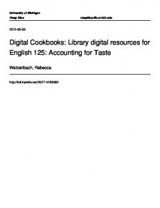
Figure 3.7: Execution time varied by applications, input size, and the number of enabled workgroups. Depending on the application and input size, the number of enabled work-groups impacts on the execution time differently.
ables. Those properties are the size of each global arguments, values of scalar arguments, the dimension of NDRange, the number of work-groups, and the number of work-items. A linear regression model requires the dependent variable y to be linear to the combination of coefficients βi and independent variables xi , but the execution time in SKMD may not be represented as a simple combination of βi and xi as described in Equation 3.1. Figure 3.7 illustrates such case since the execution time is not always linear to the number of work-groups, but becomes linear as the number of work-groups grows. Meanwhile, in some applications, the execution time also may not be linear to the input size when the input size is very small as shown in Figure 3.7(a). To handle these cases, transformations
27
are applied to independent variables as shown in Equation 3.2.
y = β0 +
n X n X m X
βk fk (xi , xj ) + ǫ
(3.2)
i=1 j=1 k=1
This equation is still a linear regression model since y is linear in the coefficients βk , but the only difference is that transformed independent variables (fk (xi , xj )) are used instead of simple xi . If modeling a linear equation is done by transforming independent variables, the prediction can also be done by plugging transformed variables into the linear equation. For the transformation, an important observation in SKMD is that the execution time eventually becomes linear to the number of work-groups when the number of work-groups is large, but the point where the linearity appears is varied by application characteristics as shown in Figure 3.7. From this property, the number of work-groups is multiplied by a function that converges from 0 to 1 as the number of work-groups increases. The tan−1 function can meet this requirement because it converges to
π 2
from − π2 . In order to make
the tan−1 function to converge from 0 to 1, the tan−1 function is divided by π and then 0.5 is added as shown in Equation 3.3, where x is the number of work-groups.
g(x) =
tan−1 (a(x − b)) + 0.5 π
(3.3)
In this equation, a is an arbitrary number that changes the slope of the tan−1 function, and b is another arbitrary number that changes the point that starts to converge. As a result of this function, the linearity to the number of work-groups will grow as the number of work-groups increases. Note that SKMD puts several transformed functions with different a and b, so the regression solver will find the best a, b values by computing the coefficients. 28
Normalized Exe. Time
Intel i7-3770
GTX 750 Ti
GTX 760
Perfect Scale
1 0.9 0.8 0.7 0.6 0.5 0.4 0.3 0.2 0.1 0
# of Work-groups
Figure 3.8: Performance impact on VectorAdd varying the number of work-groups. The execution time of GPUs do not scale down in spite of reduced number of work-groups.
To this end, a complete transformed function can be represented as Equation 3.4, where xi is the number of work-groups and xj is another independent variable.
f (xi , xj ) = xi g(xi )h(xj )
(3.4)
In this equation, the function h(xj ) is applied for the independent variable xj because the time complexity of the program may vary. For example, the time complexity of the square matrix multiplication is O(N 3 ), where N is the number of output elements. In this case, h(xj ) corresponds to xj 3 , where xj is the size of output buffer. Note that, SKMD tries various time complexity functions for h(xj ), then the linear regression solver will eventually find the best transformed function by assigning meaningful coefficient.
3.2.4 Transfer Cost and Performance Variation-Aware Partitioning Once the performance model for each device is ready, SKMD makes a decision of how many work-groups should be assigned to each device. The goal of assigning is to minimize the overall execution time by balancing workloads among several devices. This
29
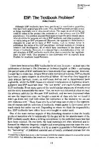
is an extension of the NP-Hard bin packing problem [18] and a common problem in load balancing parallel systems [45]. The difference is that it involves more parameters, such as data transfer time between the host and devices, and the cost of merging partial outputs. Most importantly, the performance of devices can vary as the number of work-groups assigned to devices changes. To illustrate, Figure 3.8 shows the relative execution time of the V ectorAdd kernel normalized to the time spent executing 32,768 work-groups on three devices. As shown in the figure, execution time does not scale down well as the number of work-groups decreases on discrete GPUs. If the partitioning decision is made without considering transfer cost and performance variance of partitioning, it will be suboptimal or even cause slowdown compared to single-device execution. To illustrate, the example shown in Figure 3.9 assumes that there are three external GPU devices, each of which has a different performance. If partitioning is done relying only on their maximum performance, partitioned execution may take longer than single device execution for two reasons: 1) serialized data transfer; and 2) decreased performance due to small amount of workload as shown in Figure 3.9(a). In this example, since the CPU device does not have data transfer and GPU device 2 has significant slowdown when it executes a small amount of work, more workload should have been assigned to the CPU device instead of GPU device 2. Figure 3.9(b) shows the ideal case for this example. Regarding the cost of transfer and performance variance of devices, the partitioning decision becomes a nonlinear integer programming problem. Many heuristics could potentially be used for this problem, however, one limitation is that SKMD performs partitioning at runtime, thus the algorithm must be executed very quickly so as not to overwhelm 30
Input Trans.
Kernel Exe.
Output Trans.
GPU Dev 0 Only GPU Dev 0
GPU Dev 1 GPU Dev 2
Wait
Worse on Small Work
CPU Dev
(a) Partitioning w/o considering transfer time and performance variation GPU Dev 0 Only GPU Dev 0 GPU Dev 1 GPU Dev 2
Wait Speedup
CPU Dev
(b) Ideal Partitioning
Figure 3.9: Comparison of linear partitioning and ideal partitioning
potential benefits from collaborative execution. This restriction prohibits the exact time consuming integer programming solutions [41]. To perform partitioning at runtime, SKMD utilizes a decision tree heuristic [66]. For our system, SKMD uses a top-down induction tree, where the root node is the initial status and all work-groups are assigned to the fastest device based on the estimation. A node in the tree represents a distribution of the work-groups among the devices. A node is branched to its children, and each child differs from the parent in that a fixed number of work-groups are offloaded from the fastest device to another from the parent’s partition. For each child, the partitioner estimates the execution time for all devices considering data transfer cost and performance variation of assigned work-groups. The induction is done by a greedy algorithm that chooses a child with the most time difference between offloaded device and offloading device. The partitioner traverses the tree until offloading does not decrease overall execution time.
31
Algorithm 1 Performance Variation-Aware Partitioning 1: Partition[1..k] = 0 2: BaseDev = argmin{EstDevExeT ime(x, T otalW Gs)}
⊲ Partition result of k devices
x∈k
3: 4: 5: 6: 7: 8: 9: 10: 11: 12: 13: 14: 15: 16: 17: 18: 19: 20: 21: 22: 23: 24: 25: 26: 27: 28: 29: 30: 31: 32: 33: 34: 35: 36: 37:
PrevExeTime = M in{EstDevExeT ime(x, T otalW Gs)} Partition[BaseDev] = TotalWGs ⊲ Assign all groups to base device if Contiguous Kernel then MinOffloadCnt = P artitionGranularity else MinOffloadCnt = Cnt Of f setsM ergeCost(BaseDev) end if TolerateCnt = 0 OffloadedCnt = 1 while (OffloadedCnt > 0 or TolerateCnt < 10) do OffloadedCnt = 0 CandidateDevs[1..k].TrialCnt = 0 CandidateDevs[1..k].Diff = M AX V ALU E for i = 1 to k do if Partition[i] = 0 then OffloadingTrial = MinOffloadCnt else OffloadingTrial = P artitionGranularity end if OffloadingTrial *= 2T olerateCnt if OffloadingTrial > Partition[BaseDev] then continue ⊲ Skip trial for this device end if Partition[BaseDev] -= OffloadingTrial Partition[i] += OffloadingTrial DevsTime[1..k] = EstAllDevsT ime(P artition) EstExeTime = M in{DevsT ime[0..k − 1]} if EstExeTime < PrevExeTime then CandidateDevs[i].TrialCnt = OffloadingTrial CandidateDevs[i].Diff = DevsTime[BaseDev] - DevsTime[i] end if Partition[BaseDev] += OffloadingTrial Partition[i] -= OffloadingTrial end for OffloadDev = argmax{CandidateDevs[x].Dif f } x∈k
38: OffloadedCnt = CandidateDevs[OffloadDev].OffloadingTrial 39: Partition[OffloadDev] += OffloadedCnt 40: Partition[BaseDev] -= OffloadedCnt 41: if OffloadedCnt > 0 then 42: TolerateCnt = 0 43: else 44: TolerateCnt++ 45: end if 46: end while 47: return Partition
32
In detail, the partitioner loads the linear regression equation for performance prediction for each device. The performance equations for each device are computed offline using profile data. By using the performance equation, the partitioner initially estimates the execution time for single device execution for all k devices to identify the fastest device for each kernel. The execution time in the algorithm includes the transfer cost, which can be estimated using buffer size allocated by the OpenCL APIs divided by the bandwidth of PCIe. Before the partitioner offloads work-groups from the fastest device, it determines the granularity of the number of work-groups to offload (P artitionGranularity) based on the total number of work-groups (T otalW Gs). In our framework, we limited the number of induction steps to 2,048, so P artitionGranularity becomes Ceil(T otalW Gs/2, 048). One more thing to consider in terms of offloading is the number of minimum work-groups (MinW Gs) that offsets the merge cost as a result of multiple-device execution. If the kernel is a discontiguous kernel, SKMD must merge output at the end. If the fastest device offloads work-groups to another device for the first time, the time reduced from offloading must be greater than the merge cost. The merge cost can be roughly estimated through the size of output buffer divided by the bandwidth between CPUs and the main memory. Note that the merge cost is computed only for a discontiguous kernel, while for a contiguous kernel, it uses default P artitionGranularity for initial offloading. After initial offloading, since the node in the tree contains enough work-groups to offset the merge cost already, the number of work-groups offloaded to the same device can be increased by P artitionGranularity. Once the partitioner has prepared the necessary values for traversing, it starts to traverse 33
down the decision tree from the root node by offloading P artitionGranularity workgroups to k devices at each step. At each child node, the partitioner estimates the execution time for all devices using the EstAllDevT ime function, which considers data transfer, serialization of PCIe transfer, and performance variation as a result of offloading. After the time estimation of all devices at a child node, the partitioner chooses the maximum value among estimated time, and add the merge cost to compute the overall execution time. Then, the partitioner checks if the overall execution time is reduced compared to the parent node. If a child node takes longer, it is not a candidate for the induction. If the overall time of a child node is reduced, the partitioner marks it as a candidate. For each candidate node, the partitioner computes Balancing Factor, which is the difference between the overall execution time in parent node’s and the time spent in the device that is offloaded from the parent. For the induction, the partitioner selects the candidate node with the highest Balancing Factor among all candidates. If there is no candidates, the partitioner increases P artitionGranularity temporarily to make sure that the slowdown does not come from the performance variance. If there is still no candidate after additional trials, the partitioner stops traversing and returns the status of child node which has the partitioning results. Algorithm 1 shows a high-level description of partitioning algorithm. While-Loop presented at Line 12-46 corresponds to traversing down the decision tree, and For-Loop at line 16-36 corresponds to testing children of a node in the tree. Overall, the time complexity of this algorithm is O(kN) where k is the number of devices, and N is the number of total work-groups. Note that N can be reduced to a constant by limiting the number of induction steps as described above. 34
3.2.5 Limitations As SKMD partitions workloads at a work-group granularity, global barriers or atomic operations must be handled carefully. For global barriers, the execution of work-groups should be ordered at synchronization points in the middle of execution. If work-groups are distributed across multiple devices, work-groups in each device must make sure that the other devices reached the same synchronization point. One approach to handle this case is to break down the entire kernel into multiple kernels at the global synchronization point, similar to loop fission [63], then the split kernels are executed in order. For atomic operations, the value must be updated with atomicity across all the workitems in the NDRange. However, if work-groups are scattered across multiple devices, each device will end up having their own partial atomic values. If the atomic operations are associative and commutative, intermediate atomic values from different devices can be aggregated later in the host. According to OpenCL specification, there are 11 atomic operations [37]. If an OpenCL compiler can analyze the atomic operations during compilation and detect if they are associative and commutative, OpenCL kernels can still benefit from the idea of SKMD by running special aggregation code in the runtime system. Also, kernels that have irregular behaviors may not benefit from SKMD system. The main reason is that SKMD predicts the execution time based on a regression model as discussed in Section 3.2.3, which builds a model with NDRange information, the size of array parameters, and value of scalar parameters. However, it does not consider the value of array parameters. If control flows of a kernel are heavily dependent on the value of array
35
Device
# of Cores Clock Freq. Memory Peak Perf. OpenCL Driver
Intel Core
NVIDIA
NVIDIA
i7-3770
GTX 760
GTX 750 Ti
(Ivy Bridge)
(Kepler-GK104)
(Maxwell-GM107)
4 (8 Threads)
1,152
640
3.4 GHz
1.62 GHz
1.28 GHz
32 GB DDR3 (1866)
2 GB GDDR 5
2 GB GDDR 5
435.2 GFlops
2,258 GFlops
1,306 GFlops
Intel SDK 2014
NVIDIA CUDA SDK 6.0
(Enhanced) PCIe
N/A
OS
3.0 x8 Ubuntu Linux 12.04 LTS
Table 3.1: Experimental setup.
(e.g. breath first search), the execution time is unpredictable only with the size of array. Because SKMD partitions a kernel statically before distributing work-groups, it is difficult to partition this kind of kernels optimally across several devices if the execution time is unpredictable. Applications with these semantics were not handled in this disseration, as SKMD gives up partitioning if a kernel has array-value-dependent control flows.
3.3 Evaluation SKMD was evaluated on a real machine that has three different type computing devices as shown in Table 4.1. Intel Ivy Bridge has an integrated GPU but it does not support OpenCL in unix-based operating systems, so the integrated GPU is not considered as a computing device in our experiments. However, the idea of SKMD framework is not limited to discrete GPUs. SKMD was prototyped using Low-Level Virtual Machine (LLVM) 3.4 [42], on top of a Linux system with NVIDIA driver for GPU execution, and Intel OpenCL driver for the CPU execution.
36
Every function call to the OpenCL library was hooked by our custom library that leverages SKMD’s compilation framework. Inside the framework, we used Clang for the OpenCL frontend, and LLVM 3.4 incorporated with libclc extension was used for the PTX backend [48]. However, the PTX backend is used only for Merge kernels, while Partition-Ready kernels were transformed at the source level and then directly fed into the NVIDIA OpenCL driver. Enhanced OpenCL driver for CPUs: For Partition-Ready kernels in CPUs, simply transforming a kernel at the source level and passing it to Intel OpenCL driver may cause significant overhead as discussed in Section 3.2.1. This is mainly because checking code for disabled work-groups will be executed for all work-groups within the innermost loop. To address this problem, we implemented an enhanced OpenCL driver that takes the range of enabled work-group directly so that it can selectively iterate over work-groups. In order to keep the aggressive optimizations made by the Intel driver, we used Intel’s offline OpenCL compiler that generates optimized LLVM-IRs, and then we reverse-engineered them to implement the enhanced driver that executes the generated IRs for partial work-groups. As a result of the enhanced driver, the overhead for Partition-Ready kernels is removed for the CPU. Benchmarks: For the experiments, a set of benchmarks from the AMD SDK [2] and the NVIDIA SDK [56] were used to evaluate SKMD. Some benchmarks that either do not create enough work-groups regardless of input size, or have atomic operations were excluded. Input sizes for each benchmark for the evaluation are shown in Table 3.2. The applications from the benchmark suite were compiled without any modification. In Table 3.2, Histogram and Reduction were marked as 1st round, because the OpenCL kernels 37
Application
Execution Parameters
AESEncrypt AESDecrypt BinomialOption Blackscholes BoxMuller FDTD3d Histogram (1st-round) MatrixMultiplication MatrixTranspose MedianFilter MersenneTwister Nbody Reduction (1st-round) ScanLargeArrays SobelFilter VectorAdd
4,096×4,096 BMP image 4,096×4,096 BMP image 524,288 options 32 million options 192 million numbers 3D dimsize=256, Radius=2 67 million numbers 8,192×8,192 matrices 8,192×8,192 matrices 7,680×4,320 PPM image 192 million numbers 524,288 particles 67 million numbers (float) 8 million numbers (float) 7,680×4,320 PPM image 50 million numbers (float)
Buffer Size Input Output 48 MB 48 MB 8 MB 400 MB 768 MB 68 MB 256 MB 512 MB 512 MB 128 MB 512 KB 16 MB 256 MB 32 MB 128 MB 400 MB
# of Work-groups
48 MB 48 MB 8 MB 270 MB 768 MB 68 MB 2 MB 256 MB 256 MB 128 MB 768 MB 16 MB 65 KB 32 MB 128 MB 200 MB
16,384 16,384 524,288 32,768 256 256 2,048 65,536 65,536 518,400 256 1,024 16,384 32,768 518,400 196,608
Contiguous Access N N Y Y N N N N N N N N N Y N Y
Table 3.2: Benchmark specification. VectorAdd, Blackscholes, BinomialOption, and ScanLargeArrays are classified as contiguous kernels, whereas others are defined as discontiguous kernels.
are used for generating intermediate results, and the host applications finalizes the results later. To explain Histogram in NVIDIA SDK implementation, each work-group consists of 256 work-items, and each work-item has its own 256 bins in the local memory (65,536 bins per work-group). The entire data is divided by the number of work-groups, and these chunks are split again into 256 parts for work-items. Thus, one work-item will increment its own 256 bins by inspecting one part of data. After incrementing the bins, 256 workitems are in charge of aggregating bins in the local memory. For example, work-item 0 in a work-group aggregates bin 0 of all 256 work-items, and work-item 1 gathers bin 1s, and so on. In this manner, bins for every chunk are gathered for each work-group, and these aggregations are done for all work-groups in the OpenCL kernel, which is referred to as Histogram (1st-round) in Table 3.2. With the result from the OpenCL kernel, the final aggregation is done in the second round by the host application .
38
Similarily, Reduction from NVIDIA SDK is implemented without atomic operations. Instead, work-items in a work-group reduce two numbers at the first step, and reach the local barrier. After that, half of them reduce the reduced numbers again until only one work-item remains. As a result, the last work-item will generate the reduced number for the entire work-group. These steps are done for all work-groups in the OpenCL kernel, which is also referred to as Reduction (1st-round) in Table 3.2. The reduced numbers for all work-groups are finally reduced in the second round in the host application. Methodology: Before the real execution, offline profiling is performed to collect performance data for each benchmark. For offline profiling, it is important to collect enough data to model linear regression accurately. If the model is computed with too few data, the error rate can be high especially when execution parameters of the real execution differ much from profile-run. For this reason, SKMD requires an application to use profiling mode if there is not enough profile data. With profiling mode, SKMD launches the OpenCL kernel on each device several times varying the number of work-groups. Because it is important to catch the point that linearity appears as discussed in Section 3.2.3, SKMD increases the number of work-groups by four (finer granularity) until it reaches 16, and then increases the granularity as the number of work-groups grows. Once profile data is collected, SKMD performs the linear regression analysis as discussed in Section 3.2.3. For the dynamic overheads, we did not consider the cost of kernel analysis and transformation because they can be done during offline profiling, but we measured the partitioning overhead, which is done in the real execution. To reduce the overhead, we forced the height of decision tree used in partitioning algorithm to be within 1,024 steps. In other words, for kernels that launch more than 1,024 work-groups, SKMD increases partitioning granular39
ity. As a result, 1, 024 × 2 (the number of offloading devices) estimations are done in the worst case. As 2,048 time estimations can be done with less than 100K instructions, the overhead for the partitioning algorithm is observed as less than 1ms which is negligible for all benchmarks. We measured wall clock execution time including the transfer time between host and GPU devices, kernel execution time, and data merging cost in case of discontiguous access kernels. Because the CPU resource is shared with the operating system or other applications, the execution time on the CPU device can vary. Therefore, we ran 1,000 times for each benchmark and selected 100 sets of results that have the least CPU execution time, and used the average of those 100 results for the final result.
3.3.1 Results and Analysis Figure 3.10(a) shows speedup of SKMD compared to the fastest single device execution and the linear partitioning execution, which is similar to prior approaches [49, 38]. In the linear partitioning, the number of work-groups assigned to each device are proportional to the predicted performance without consideration of the transfer cost. The baseline is different for each benchmark based on its characteristics. For each benchmark, we ran them on all devices and chose the fastest device (including the transfer cost) as the baseline. Three benchmarks, Reduction, Histogram, and VectorAdd used CPU-only execution as their baseline because data transfer cost overwhelms the benefits of executing on GPUs, as they are extremely memory-bound kernels. As illustrated in Figure 3.10(a), SKMD performs 28% faster than the single device execution on average as it considers the transfer cost and performance variation of each 40
GTX 750 Ti Only
Intel i7-3770 Only
GTX 760 Only
Linear Partition
SKMD Partition
2.5 2 1.5 1 0.5
Discontiguous Kernels
Contiguous Kernels
GEOMEAN
GEOMEAN
ScanLargeArrays
BinomialOption
BlackScholes
VectorAdd
GEOMEAN
SobelFilter
MedianFilter
Nbody
FDTD3d
AESDecrypt
AESEncrypt
BoxMuller
MersenneTwister
MatrixTranspose
MatrixMultiplication
Histogram
Reduction
0
ALL
(a) Speedup normalized to the fastest single device execution GTX750Ti Linear Partition
GTX760
Intel i7-3770
SKMD Partition
Discontiguous Kernels
Contiguous Kernels
AVERAGE
ScanLargeArrays
BinomialOption
BlackScholes
VectorAdd
SobelFilter
MedianFilter
Nbody
FDTD3d
AESDecrypt
AESEncrypt
BoxMuller
MersenneTwister
MatrixTranspose
MatrixMultiplication
Histogram
Reduction
100% 90% 80% 70% 60% 50% 40% 30% 20% 10% 0%
-
(b) Work-group distribution
Figure 3.10: Speedup and work-group distribution. Each benchmark has different baseline (a), as the fastest device differ by kernels. The fastest device is determined with regard to the execution time and data transfer cost.
device during partitioning. An important point from this result is that the linear partitioning causes slowdown on memory-bound kernels compared to the single device execution. This is mainly because it does not take the transfer cost into account during the partitioning although collaborative execution is not favorable due to the transfer cost.
41
To illustrate how SKMD partitions work-groups across different devices, Figure 3.10(b) shows the work distribution of all applications. On average, SKMD partitioning, which considers the transfer cost, assigns more workload to the CPU than the linear partitioning. The linear partitioning makes a bad decision for memory-bound applications by assigning less workload to the CPU, although considerable amount of time is spent on transferring the data. On the other hand, SKMD partitioning assigns more workload to the CPU, as the CPU can work more while the data is being transferred to the external GPUs. Reduction, Histogram, VectorAdd: Reduction, Histogram, and VectorAdd are extremely memory-bound kernels so SKMD assigns most of the work to the CPU device. The difference is that Reduction and Histogram are recognized as a discontiguous kernel, so the host program must transfer the entire input to the external GPU device which discourages collaborative execution due to expensive cost of data transfer. On the other hand, VectorAdd which is a contiguous kernel does not require the entire input for the partial execution, so there is still a chance for the CPU to offload work-groups to the GPU devices. MatrixMultiplication, AESEncrypt/Decrypt, Nbody, BinomialOption: These benchmarks are compute-bound kernels where a significant amount of time is spent on computation, not memory accesses. For these benchmarks, the portion of the workload assigned to the GPUs are higher than the CPU because of its massively data-parallel structure. As mentioned earlier, because GTX 760 is a high performance GPU, it executes more work-groups than GTX 750 Ti. MatrixTranspose: MatrixTranspose is a memory-bound kernel but SKMD assigns all of work to GTX 750 Ti despite the expensive cost of data transfer. This is due to the very low performance of the CPU. Since the OpenCL implementation targets GPUs, each work42
group has a local memory to store input in order to avoid un-coalesced global memory accesses among work-items. However, for the CPU execution, having local memory does not benefit from coalesced memory access, but rather produces unnecessary overhead of copying data to additional space. This overhead may not be significant for other benchmarks, but for MatrixTranspose in the CPU, copying input to the scratchpad is another equal amount of work compared to the naive transpose. ScanLargeArrays: ScanLargeArrays has large memory foot-prints with contiguous memory access patterns. Similar to VectorAdd, it does not have to transfer the entire data back and forth between the CPU and the GPUs. However, it has more computations than VectorAdd that are faster on GPUs, so larger portion of workload is offloaded to the GPUs than VectorAdd. Other benchmarks have considerable amount of computations and large memory footprints with discontiguous access patterns. In this case, both compute and transfer costs are proportional to the size of data, so the data transfer time could offset the reduced computation time from the collaborative execution. As a result, the speedup from the collaborative execution is relatively low as shown in Figure 3.10.
3.3.2 Execution Time Break Down In this section, we show how SKMD transfers data between the CPU and the GPUs, and assigns work-groups to different devices. Figure 3.11 shows the execution time break down of three sample applications: Vector Add, Matrix Multiplication, and Histogram. For VectorAdd, CPU-only is the baseline because it is an extremely memory-bound kernel. As shown in Figure 3.11(a), SKMD starts the execution on the CPU while trans43
SKMD Partitioning Intel
Input Transfer
Kernel Execution
Output Transfer
Merge Time
Only GTX 750 Ti GTX 760
Intel i7-3770
0
5
10
15
20 25 Time(ms)
30
35
40
45
(a) VectorAdd
GTX SKMD Partitioning 760
Input Transfer
Kernel Execution
Output Transfer
Merge Time
Only GTX 750 Ti GTX 760
Intel i7-3770
0
1000
2000
3000 4000 Time(ms)
5000
6000
7000
(b) MatrixMultiplication
SKMD Partitioning Intel
Input Transfer
Kernel Execution
Output Transfer
Merge Time
Only GTX 750 Ti GTX 760
Intel i7-3770
0
5
10
15
20 Time(ms)
25
30
35
40
(c) Histogram
Figure 3.11: Break down of the execution time on each device. The bars on the top is the baseline, which is the fastest single-device execution. SKMD considers the transfer cost, and offloads workgroups in order to balance the workload among the three devices.
ferring huge data to GTX 760 in background. As soon as the data transfer is finished, SKMD launches the kernel on GTX 760, and at the same time, it transfers data needed for the remaining work-groups to GTX 750 Ti and then launches the kernel. The transfer time for GTX 750 Ti is smaller because it is a less powerful GPU for VectorAdd so the size of data assigned to it is smaller. Since VectorAdd has contiguous memory accesses, there is no need to merge the data. After both kernels are done, the buffer manager transfers the
44
data from the GPUs and simply puts them in the final result. As shown in the figure, the CPU finishes execution almost at the same time as the GPUs finish their data transfer as a result of accurate partitioning. The baseline of MatrixMultiplication is GTX 760-only as shown in Figure 3.11(b). Since Matrix Multiplication takes much more time in computation than VectorAdd, the impact of transferring time is less for this benchmark. However, SKMD transfers the entire input and output back and forth between the host and GPU devices as it is classified as a discontiguous kernel. Similar to VectorAdd benchmark, GTX 760 starts execution first followed by GTX 750 Ti but finishes later than GTX 750 Ti because it has more workgroups to execute due to its higher performance. At the end, the CPU merges all partial results to generate the final output by launching the merge kernel. Histogram shows different behavior from the other cases. The baseline for Histogram is CPU-only execution because it has large input, which incurs large transfer cost for the GPU execution. In terms of execution performance, GTX 750 Ti outperforms than GTX 760 for Histogram as shown in Figure 3.10(b)-Linear Partition, which partitions kernels linear to the performance. Therefore, GTX 750 Ti has higher priority for offloading. Also, the output size is much smaller than input size as shown in Table 3.2. Histogram is categorized as a discontiguous kernel, so SKMD still has to transfer the entire input to the external GPU devices. As shown in Figure 3.11(c), SKMD does not assign any work-groups to GTX 760 after assigning some work-groups to GTX 750 Ti, because serialized input data transfer to GTX 760 would break balanced execution among three devices. As the output size is small, the overhead of merging kernel is negligible for this benchmark. 45
Application AESEncrypt AESDecrypt BinomialOption Blackscholes BoxMuller FDTD3d Histogram (1st-round) MatrixMultiplication MatrixTranspose MedianFilter MersenneTwister Nbody Reduction (1st-round) ScanLargeArrays SobelFilter VectorAdd
Profile Parameters Profile 1
Profile 2
Real Parameters (same as Table 3.2)
1,024×1,024 BMP image 1,024×1,024 BMP image 16,384 options 1 million options 8 million numbers 3D dimsize=64, Radius=1 4 million numbers 1,024×1,024 matrices 1,024×1,024 matrices 1,920×1,080 PPM image 8 million numbers 65,536 particles 8 million numbers 500,000 numbers 1,920×1,080 PPM image 8 million numbers (float)
2,048×2,048 BMP image 2,048×2,048 BMP image 65,536 options 8 million options 32 million options 3D dimsize=128, Radius=2 16 million numbers 2,048×2,048 matrices 2,048×2,048 matrices 3,840×2,160 PPM image 64 million numbers 131,072 particles 34 million numbers 1 million numbers 3,840×2,160 PPM image 16 million numbers
4,096×4,096 BMP image 4,096×4,096 BMP image 524,288 options 32 million options 192 million options 3D dimsize=256, Radius=2 67 million numbers 8,192×8,192 matrices 8,192×8,192 matrices 7,680×4,320 PPM image 192 million numbers 524,288 particles 67 million numbers 8 million numbers 7,680×4,320 PPM image 50 million numbers
Table 3.3: Profile execution parameters and real execution parameters for evaluating performance prediction accuracy. For each profile, 16 profile data was collected varying the number of workgroups.
3.3.3 Performance Prediction Accuracy To evaluate the accuracy of performance prediction on the CPU and the GPUs, we profiled the applications with two sets of execution parameters as shown in Profile Parameters of Table 3.3. With the profiled data from two sets of execution parameters, SKMD performed a linear regression analysis to get the coefficients. After the computation of the coefficients, we ran the applications with the real execution parameters as shown in Real Parameters Table 3.3. For the real execution, we randomly picked the number of partial work-groups 128 times, and compared the real execution time with the predicted execution time. Figure 3.12(a) shows the L2-Norm errors between predicted time and execution time, and Figure 3.12(b) shows the average error rate for each benchmark. The L2-Norm error means Euclidean distance between two time vectors, thus it represents the amount of error
46
Intel i7-3770
GTX 750 Ti
GTX760
0.14
0.12
(ms)
0.1
0.08 0.06 0.04 0.02 0
(a) L2-Norm Intel i7-3770
GTX 750 Ti
GTX760
3.0% 2.5%
Rate
2.0% 1.5% 1.0%
0.5% 0.0%
(b) Average Error Rate
Figure 3.12: Performance prediction accuracy. L2-Norm error (a) shows Euclidean distance between the real execution time and the predicted execution time in milliseconds. Average error rate (b) shows the average percentage of errors in predictions.
in milliseconds, while the average error rate shows the difference over the real execution time. For all benchmarks, high error ratios were observed when SKMD predicts the execution time with a very few number of work-groups. This is mainly because the execution time is very short with a few number of work-groups. As a result, even small error values can result in high error ratios. For example, if SKMD predicted the time as 0.011 ms, but
47
the real execution took 0.01 ms, then the error ratio becomes 10% in spite of only 0.001 ms of misprediction. Considering that the execution time for the execution parameters shown in Table 3.3 takes more than 10 ms for all benchmarks, the errors in prediction time are negligible since the error remains under 0.1 ms in most cases as shown in Figure 3.12(a).
3.4 Related Work A significant focus has been on the execution of data-parallel applications on CPUs. [46] examined several data parallel applications to show that CPUs can have comparable performance to GPUs, if it takes full advantage of multi-cores with single instruction multiple data (SIMD) units. There has also been some work on efficient execution of OpenCL/CUDA applications on CPUs. [75] proposed a source-to-source compiler that translates a CUDA program into a standard C program using loop-fission technique to eliminate synchronization. Similarly, [12] developed the Ocelot, a runtime system that dynamically transforms OpenCL/CUDA kernels for CPU execution. [24] also performed a similar study, but approached in a light-weight thread (LWT) execution model. In a similar fashion, [33] has focused on more efficient execution of OpenCL applications using whole-function vectorization. All of these prior works are focusing on performance improvement on CPUs to show CPUs can perform as good as GPUs for some applications but none of them deals with collaborative execution with GPUs. Performance modeling of GPUs for a certain set of applications have been studied for several years [31, 25]. [25] proposed an analytical model for a GPU architecture with awareness of memory-level and thread-level parallelism. However, this model relies only
48
on static information of GPU architectures and applications, such as the number of registers, the size of memory on the device and those numbers required by the application. Also, this study was based on relatively simple GPU architectures compared to contemporary GPU architectures, which is much harder to predict the performance statically. Meanwhile, Jia et al. proposed a GPU performance prediction method based on a linear regression model, but the work used the prediction model for GPU space exploration varying GPU architectures. On the other hand, our work described the linear regression model that fits for various execution parameters in order to optimize the performance. Dynamic decision of execution on heterogeneous systems with CPUs and GPUs has been studied in the past [13, 47, 49, 7, 36]. Harmony [13] reasons about the whole program by building a data dependency graph and then scheduling independent kernels to run in parallel. However our approach is different from prior works in that our system is working on finer granularity (work-groups) rather than function or task level. MERGE [47] is a predicate dispatch-based library system for managing map-reduction applications on heterogeneous systems. [49] proposed the Qilin that automatically partitions threads to one CPUs and one GPUs by providing new APIs that abstract away two different programming models, Intel Thread Building Block and CUDA. [38] also proposed a framework that distributes workload of an OpenCL kernel to multiple equivalent GPUs for specific types of data-parallel kernels. Delite [7] and is a compilation framework that takes a program written in OptiML and converts it into C++/CUDA program. Then runtime system manages execution between CPU and GPUs. While this work is limited to domain-specific languages, SKMD provides more generality as it supports a variety of OpenCL applications. The PEPPHER proposed by [36] improved the performance by tuning the execution 49
strategy on a heterogeneous system based on their performance prediction model. Our approach differs from prior work in that our system supports more than two different types of devices and considers data transfer cost and performance variance during partitioning. Also, our approach does not rely on additional programming extensions or APIs. In the mean time, a series of works have been done for virtualizing GPU resources [67, 34, 68, 79, 76, 43]. PTask [67] provides APIs that work with OS abstraction layers to manage compute tasks on GPUs by using a data-ow programming model. Dandelion [68] also proposes a compiler/runtime framework that takes C# sources with newer APIs, and converts them to CUDA code, and runtime manages execution between CPUs and GPUs using PTask [67]. [34] proposed Gdev that manages GPU resources in the OS level, so GPUs can be treated as first class computing resources in multi-tasking systems. SKMD is different from these prior works as SKMD does not require programmers to use additional APIs or language extensions, but it is transparent to OpenCL applications, which can be further optimize parallel kernels by utilizing local memories. [79, 76] also proposed virtualization layers for GPUs which take over the control of GPU memory space from applications without changing APIs. Through these techniques, GPUs can access the data in the host directly on page faults. Similarly, NVIDIA recently offered Unified Virtual Address to provide abstract view of unified memory system in separate physical memory [58]. Main purpose of this idea is removing the burden of managing multiple memory spaces [35], but it still leaves work distribution between devices as programmer’s responsibility. On the other hand, SKMD focuses on balancing workloads across multiple computing devices and transfers the entire working-sets at once in order to avoid high overhead from frequent PCIe bus transactions for page fault handling. 50
3.5 Conclusion In this chapter, we presented SKMD, a framework that transparently manages collaborative execution on CPUs and GPUs of a single OpenCL kernel. SKMD leverages assigning a subset of data-parallel workload over multiple CPUs and GPUs so as to increase overall performance. As a part of the exploration, this chapter introduced several techniques that transparently enable a kernel to work on a partial workload and efficiently merge results from separate devices. In order to distribute a balanced workload, this chapter also presented an accurate performance prediction model and an efficient methodology for balancing workload between CPUs and GPUs being aware of data transfer cost and performance variance depending on the type of device. By experimenting with OpenCL applications on a real hardware, we showed that SKMD yields a geometric means of 28% speedup on a machine with one CPU and two different GPUs as compared to the fastest device-only execution.
51
CHAPTER IV
VAST: Virtualizing Address Space for Throughput Processors
4.1 Introduction Graphics processing units (GPUs) have emerged as the computational workhorse of throughput oriented applications because of their low cost, high performance, and wide availability [8]. Modern GPUs achieve several tera floating point operations (FLOPS) of peak performance while costing a few hundred dollars. With CUDA or OpenCL, programmers can develop data parallel kernels for GPUs that achieve speedups of 4-100x over traditional processors (CPUs) [69]. As a result, software in various domains has been connverted to exploit GPU’s computing resources, many of which work on large data sets. For example, galaxy formation simulation in space research computes physical forces among hundreds of million particles [74]; economical analysis combines thousands of factors in tens of dimensions and then computes on it [15]; and numerous fields perform data minings from a huge amount of data [80], 52
However, discrete GPUs have a critical limitation: the entire data to process must reside in GPU memory before execution. When the data size exceeds the physical memory of the GPU, the application should be developed to let the GPU to access the host memory directly through the peripheral component interconnect express (PCIe) bus for every access, which has much lower bandwidth and higher latency than GPU’s memory. Otherwise, the execution must be fallen back to the CPU which supports nearly arbitrary data sizes through virtual addressing. Smart programmers can overcome this restriction by applying a divideand-conquer approach. In this case, the programmer explicitly divides the workload into smaller chunks and executes a series of kernels each processing a subset of the data. This approach is not a panacea, however. Even in the simple case where the kernel operates on contiguous data chunks, explicit data management is tedious, requiring manual buffer allocations and data transfer to/from the host. For non-contiguous data, divide-and-conquer is more complex. Lastly, the size of chunks may change across GPUs with differing amounts of physical memory. A natural question is why do GPUs not support virtual addressing to eliminate this problem as CPUs have done for many decades [71, 5]. Through a combination of hardware (e.g., translation look-aside buffers) and operating system support (e.g., page tables), CPUs provide the appearance of a nearly infinite address space to facilitate processing large data sets. However, virtualizing the address space of discrete GPUs is difficult for the following reasons: • Discrete GPUs have separate memories that use different address spaces, and each transaction between the host and GPU is expensive.
53
• GPUs do not interact with the operating systems for memory management, but instead directly access their physical memory. • Execution on GPUs is non-preemptive, therefore all data must be present in the physical memory before execution. The combination of these factors makes it difficult to execute kernels on GPUs whose total memory footprint exceeds the physical memory size on the GPU without programmer intervention. As the size of data to process keeps increasing, this limitation will become more significant. To tackle these challenges, we present Virtual Address Space for Throughput processors (VAST), a run-time software system that provides the programmer with the illusion of a virtual memory space for commodity OpenCL devices. VAST transparently divides and transfers working sets based on the available physical memory space on the target GPU. To virtualize the memory space, VAST adopts a look-ahead page table (LPT), a new type of page table that contains a list of virtual pages that will be accessed by specific ranges of the OpenCL workload. LPT differs from conventional page tables used in operating systems in that the LPT is filled up before the pages are actually accessed. With LPT, VAST decomposes the working set into individual page frames for execution of the partial workload. Page frames are packed into a contiguous buffer (frame buffer) that resides in the GPU’s physical memory and LPT represents the mapping of an OpenCL buffer from the CPU’s virtual space into the GPU’s physical space (the frame buffer). Instead of transferring the entire data to the GPU, VAST transfers the LPT and frame buffer for each partial workload. At the same time, VAST transforms the kernel to access memory through
54
the LPT (e.g., software address translation). The VAST runtime system significantly improves GPU portability as it can utilize any GPU for larger sized workloads. The challenges of VAST are four fold: dividing an arbitrary workload based on the available physical memory size, efficiently generating the LPT and frame buffer, transforming the kernel to use the relocated and packed data, and avoiding replicated transfers due to reuse of data across partial workloads. To address these issues, this dissertation makes following contributions: • A code transformation methodology that quickly inspects memory access locations of an OpenCL kernel in order to generate LPTs. • A novel technique that partitions an OpenCL workload into partial workloads based on the physical memory constraints of a GPU and packs the corresponding data into a frame buffer using LPTs. • Kernel transformation techniques to access data out of the frame buffer using LPTs. • A technique to avoid replicated data transfers to the GPU. • A comprehensive performance evaluation of VAST on real hardware consisting of an Intel Core i7 3770 CPU and an NVIDIA GTX 750 Ti GPU. The rest of the chapter is organized as follows. Section 4.2 discusses the OpenCL execution model and opportunities for virtualizing GPU memory space. Section 4.3 explains the overview of VAST, and then the implementation and optimizations are discussed in Section 4.4 and Section 4.5 respectively. The experimental results of using VAST for various OpenCL applications are presented in Section 4.6. Section 4.7 discusses the related 55
__kernel void matrixMul(__global float* C, __global float* A, __global float* B, int wA, int wB, int range_from, int range_to) { int gid_x = get_group_id(0); int gid_y = get_group_id(1); int size_x = get_num_groups(0); int flat_id = gid_x + gid_y * size_x; // check whether to execute if (flat_id < range_from || flat_id > range_to) return; int idx = get_global_id(0); int idy = get_global_id(1); float value = 0; for (int k = 0; k < wA; ++k) { value += A[idy * wA + k] * B[k * wB + idx];_________ } C[idy * wA + idx] = value; }
Figure 4.1: The code transformation for partial execution of an OpenCL kernel. The kernel takes two additional arguments for the work-group range to execute, and grey backgrounded code is also inserted at the beginning of the kernel to check if the work-group is to be executed. The work-groups out of the range will terminate the execution immediately.
work in this area. And finally, we conclude in Section 4.8.
4.2 Motivation As discussed in Chapter II, an OpenCL kernel can be executed in parallel at a workgroup granularity without concern of the execution order. Through the code transformation, the OpenCL host program can control the number of executed work-groups as shown in Figure 4.1. By inserting checking code at the beginning of the kernel, every work-item checks if the work-group it belongs to is supposed to execute. If it should not, the workgroup terminates the execution immediately and the GPU will schedule it out. In this way, we can limit the total amount of memory accessed by those work-groups to a predefined amount (the GPU’s physical memory size). This memory is reorganized into page frames
56
and packed into a frame buffer by VAST. A look-ahead page table (LPT) is then used to map between the original CPU address to the page frame address for the GPU. We refer to this model as partial execution and the goal of VAST is to automate the decomposition and to restrict the kernel as necessary to realize software-managed paging.
4.3 VAST System Overview VAST is an abstraction layer located between an application and the OpenCL library. The VAST layer overloads all OpenCL APIs including device-querying functions. By overloading device-querying APIs, VAST provides the application with the illusion of a virtual GPU device that has very large amount of memory. With the virtual device, programmers can allocate buffers as much as they need without concern for the physical memory size. In order to virtualize address space of OpenCL kernels, actual data must be rearranged into page frames with the look-ahead page table (LPT), which is filled with a list of pointers to the corresponding page frames that will be accessed during the execution. In addition, the OpenCL kernel must access data through the LPT and frame buffer (address translation), as similar to the conventional program accessing data through TLBs and the operating system’s page table. After kernel execution, the output buffer for the LPT and page frames must be recovered to original memory space on the host. The rest of this section describes execution flow of VAST system and illustrates timeline of VAST execution.
57
Application OpenCL Kernel
VAST System x86 Code
Look-ahead Page Table Generator
1 Transform
IR
PTX Code 2 Inspector
Array Recovery
7
Kernel
CPU
Paged Access Kernel
OpenCL Library GPU
Plain Array
4
S
...
10 Recover
...
Addr MSB 0x0000 0x0001 0x0002
5 LPTgen
0xFFFF Frame Buffer ...
PAS 0 1 1 ... 0
0: Not used 1: Used
6 S
LPT 0 ...
3 PASgen
9
1023
8 Execute
S
Host Memory
GPU Memory
Figure 4.2: The VAST system located between applications and OpenCL library. VAST takes an OpenCL kernel and transforms it into the inspector kernel and the paged access kernel. At kernel launch, the GPU generates PASs (P ASgen) by launching the inspector kernel, then transfers them to the host to create LPT and frame buffer (LP T gen). Next, LPT and frame buffer are transferred to the GPU in order to execute the paged access kernel.
4.3.1 VAST System Execution Flow Figure 4.2 illustrates sequences of VAST system operations. First, VAST compiles an OpenCL kernel into intermediate representations (IRs), and then generates a GPU binary
58
(PTX) for the Inspector Kernel, and the Paged Access Kernel as shown in Figure 4.2 ➊. After a compilation request, the application will request the kernel launch. On this request, VAST first launches the Inspector Kernel ➋ that only inspects usage of global arguments (arguments with global keyword) and fills up the Page Accessed Sets (PASs) ➌. PAS contains boolean values that represent whether a work-group has accessed each page. Note that each work-group has its own PAS for each global argument of the kernel, and the ) where AllocSize is actual OpenCL buffer allocation size of PAS is fixed as Ceil( PAllocSize ageSize size from the application. For example, 4GB of OpenCL buffer will require 1MB of PAS with 4KB pages. In order to reduce the number of PASs, one PAS can be shared among several work-groups. In this case, one PAS represents the pages accessed by a subset of work-groups. Next, VAST transfers PASs from the GPU to the host ➍, and then the host fills up the LPT and frame buffers using the PASs until the size of frame buffer reaches the available GPU memory size ➎. After that, VAST allocates the actual buffers for the LPT and frame buffer on the GPU, and transfers them to the GPU device ➏. At this point, VAST knows how many work-groups should be executed as it has generated the LPT and frame buffer for the specific range of work-groups. In order to execute specific range of work-groups of the kernel, the Paged Access Kernel also takes additional parameters for the ranges of work-groups to execute as discussed in Section 4.4.2 of Chapter III. Once VAST finishes the transfer, it launches the Paged Access Kernel ➐, which accesses the memory through the LPT. During execution, the frame buffer in the device memory will be updated ➑, and after the execution, VAST will transfer them back to the host memory space ➒. Finally, VAST 59
PAS gen
Gathers Frame Buffers for k work-groups
A
depends on
B
LPT gen w/ Frame Buffer
*
Transfer Host to Device Paged Access Kernel Execution Transfer Device to Host Array Recovery
Time
Figure 4.3: Execution timeline for VAST system. Only PAS generation and the first LPT generation cost is exposed. Other LPT generations and array recoveries are overlapped from data transfer and kernel execution. With double buffering, the second LPT generation starts immediately after the first LPT generation.
recovers arrays using the LPT and modified frame buffer ➓, and repeats the steps from LPT generation ➎ to recovery ➓ until all work-groups finish their execution.
4.3.2 VAST Execution Timeline Figure 4.3 visualizes the timeline of VAST execution. As shown, the cost of generating LPTs and frame buffers can be hidden by overlapping them with data transfer and kernel execution. Thus, the only exposed cost is PAS generation and the first LPT generation. Mind that VAST allocates LPTs and frame buffers twice on the host for double buffering. With double buffering, the next LPT generation can proceed right after the previous LPT generation, as shown in Figure 4.3. One important point from Figure 4.3 is that transferring the second working set to the GPU (marked as * ) starts after retrieving the first partial result back to the host, not after the kernel execution. The main reason is that some pages written in the first partial execution can also be written by the work-groups in the second partial execution. Similar to data for-
60
warding in a CPU pipeline datapath, VAST forwards only written pages from the previous execution to the next execution. Details of forwarding shared pages will be discussed in Section 4.4.4. Another feature of VAST is that it avoids duplicated data transfer. To illustrate, if page frames of a global argument during the partial execution are identical to that of the next execution, VAST skips LPT and frame buffer generation as well as buffer transfer for the next execution.
4.4 Implementation This section discusses the implementation of VAST system including design of PAS, kernel transformations, and how to create LPT and frame buffers using PASs. Also, the ways to handle shared pages and to avoid duplicated data transfers are discussed.
4.4.1 The Design of Page Accessed Set As described in Section 4.3.1, the first step for VAST is launching the inspector kernel on the GPU in order to generate Page Accessed Sets (PASs). PAS represents a list of pages accessed by a set of work-groups during execution. Therefore, each entry of PAS contains a boolean value as shown in Figure 4.4. Later, these PASs will be used on the host to generate Look-ahead Page Table (LPT), which contains pointers to the page frames. The inspector kernel is able to execute on the GPU without transferring the working set because most OpenCL kernels use a combination of work-item index and scalar variables as the index of global array access. Upon this property, VAST passes only scalar and
61
-
float value = argK[Offset];
Table Index
log2PAGESIZE - log2TYPESIZE
0 1 0 ...
...
...
PAS for Work-group N
0 PASs for arg1
PASs for argK
PAS of argK for work-group N
Figure 4.4: The design of Page Accessed Set (PAS). Each work-group has its own PAS for each global argument. Each entry of PAS has a boolean value that represents whether corresponding page has been accessed by the work-group.
constant arguments to the inspector kernel along with the NDRange information (size of work-groups and work-items) for PAS generation. If global array access depends on the value of a global argument, (e.g. indirect memory access), the inspector code is leveraged on the host, and the host generates PASs directly. As shown in Figure 4.4, VAST makes use of single level paging because it minimizes both PAS generation time for the inspector kernel and address translation time for the paged access kernel. As a result, with 4KB pages, 4 GB of data can be fit into 1 MB of PAS if each entry uses 1 byte to store a boolean value. However, if PASs are maintained per workgroup per global argument, the size of overall PASs can become significant if the kernel is launched with a large number of work-groups. For this reason, VAST makes a set of consecutive work-groups to share one PAS depending on the number of work-groups. The
62
number of work-groups per PAS is determined statically using the equation below. W ORKGROU P P ER P AS = Ceil(
M EM SIZE 32 AllocSize T OT AL W ORKGROU P
)
(4.1)
The assumption behind this equation is that one work-group accesses the space of AllocSize . T OT AL W ORKGROU P
not to exceed
With this assumption, VAST computes the number of work-groups
M EM SIZE 32
accesses. This is a rough estimation, and if it appears that the
number is too small or large, VAST adjust the number dynamically. When several work-groups try to modify the shared PAS, atomic operation is not necessary because according to NVIDIA’s programming guide [58], if a non-atomic instruction executed by more than one thread writes to the same location in global memory, only one thread performs a write and which thread does it is undefined. Thus, it is safe to share one PAS among several work-groups and work-items because every work-item will try to write the same boolean value (TRUE).
4.4.2 OpenCL Kernel Transformation As shown in Figure 4.2 - ➊, VAST transforms each OpenCL kernel into an inspector kernel and paged access kernel. Both kernel transformations only focus on usages of global arguments, but the difference is that the inspector kernel replace entire memory operations with the new stores, while the paged access kernel replaces only the bases and offsets of memory operations as shown in Figure 4.5. In detail, the first step for the inspector kernel transformation is to inline function calls in the kernel in order to avoid expensive inter-procedural analysis. In general, every function call can be inlined since the OpenCL programming model prohibits recursive calls as it
63
offset
offset 5 Remove dead code
1
SHIFT AMT
Get LPT base
SHIFT AMT SHR (>>)
&LPT
Get
SHR (>>)
2
2 PAS Index
&arg1
Get LPT Index
AND 3
LD 4
1
SHIFT MASK
Get PAS base
LOAD Frame Index
&Frame Buffer
&PAS
Get Frame Offset
SHL (