Virtuous interactions in removing exclusion: the link between ... - Aiccon

FACOLTA’ DI ECONOMIA UNIVERSITA’ DI BOLOGNA SEDE DI FORLI

Percorso di Studi in Economia Sociale

Virtuous interactions in removing exclusion: the link between foreign market access and access to education Leonardo Becchetti Pierluigi Conzo Fabio Pisani

Working Paper n.63 Luglio 2009 in collaborazione con

Leonardo Becchetti, Pierluigi Conzo, Fabio Pisani, Università di Roma Tor Vergata

Informazioni Facoltà di Economia – Percorso di Studi in Economia Sociale Tel. 0543 374673 - Fax 0543 374660 – e mail: [email protected] Web: www.ecofo.unibo.it

Virtuous interactions in removing exclusion: the link between foreign market access and access to education Leonardo Becchetti, University of Rome Tor Vergata Pierluigi Conzo, University of Rome Tor Vergata Fabio Pisani, University of Rome Tor Vergata

Abstract We devise a retrospective panel data approach to evaluate the effects of fair trade affiliation on the schooling decisions of a sample of Thai organic rice producers across the past 20 years. We find that the probability of school enrolment in families with more than two children is significantly affected by affiliation years. The finding is robust when dealing with endogeneity and heterogeneity issues in the estimate. The nonpositive preaffiliation performance documents that our result is not affected by selection bias and that fair trade affiliation generates a significant break in the schooling decisions of affiliated households.

Keywords: child schooling, market access, fair trade. JEL numbers: O19, O22, D64.

2

1. Introduction

It is common sense to expect a negative relationship between the number of children and children education for poor households in LDCs. The causal link between the two variables depends on the fact that families should decide jointly the number of children they want and the level of education to give them. For a given budget constraint, the higher the number of children, the lower the investment in available per child education (Becker and Tomes, 1976). On this basis a causal relationship between number of children and probability of going to school may arise in case of an exogenous increase in family offspring.1 The goal of this paper is to verify whether in situations in which the quality (of education)/quantity trade-off is expected to matter (among agricultural producers in LDCs close to the poverty line), the trade-off may be eased by policies which affiliate producer cooperatives to organisations - such as those of fair trade (henceforth also FT) importers - which promote producers’ access to export markets and pay them a premium which has to be invested in both local public goods and capacity building.2 The direction of the impact of such policies on child schooling is not so straightforward. On the one side, the Basu and Van (1998) luxury axiom states that parents decide to send their children to school when they overcome a minimal household income threshold which allows them to afford such cost. The income effect of such premium should have undoubtedly a positive impact on child schooling if it brings the household beyond such threshold. On the other side, however, the 1

Recent empirical contributions (Booth and Kee, 2009; Iacovou, 2001) show that education is negatively correlated with family size and birth order. The trade-off between quantity and quality is also supported by findings from Hanushek (2002), Steelman and Powell (1989), and Yilmazer (2008), the last two works showing that in large families there are less financial resources for school fees. On the other side Black et Al. (2005) find a relationship between birth order and school attainment where family effects are not significant, so that the determinants are differences within families and not only across families. For a more general survey on related issues in the child labour literature see among others Deb and Rosati (2002) and Bhalotra and Heady (2003). 2 A detailed description of the producer cooperative (GreenNet) and of the partner organisation promoting access to export markets (fair trade), object of our empirical analysis, will be provided in the next section. 3

substitution effect of the price premium paid by the fair trade organisation tells us that the opportunity cost of school investment is higher since one hour of child work in the household agricultural activity yields more. In addition to it, additional indirect changes in affiliated and non affiliated producer labour markets in a general equilibrium framework should also matter and be taken into account in the evaluation of the total impact. Our empirical analysis aims to evaluate the direction of such effect. Another main task of the paper is to disentangle, for what possible, causal links from two endogeneity problems which arise when dealing with the above mentioned issue. On the one side, the same quality/quantity trade-off may conceal a third driving factor (i.e. low parents’ endowment in terms of ability, wealth and education) which affects both the decision to have more children and to invest less in them (PonceSouza, 2009). On the other side, the relationship between affiliation to FT and child schooling may also be spurious and driven by selection bias. A final added value in our paper is methodological and lies in the definition of a simple and effective retrospective panel data approach. The latter helps to investigate issues in which repeated observations on the same sample of individuals for many years are too costly or, if not started in advance, make just impossible an impact analysis. With this respect we devise a very simple approach which allows to build retrospectively panel data without requiring unreasonable memory efforts by repondents. Differently from McIntosh et al. (2010) who look at house restructuring events, we build our retrospective panel data on simple questions about children age and schooling years allowing us to reconstruct the pattern of household schooling decisions over a long time interval.

The paper aims to deal with all these issues and is divided into eight sections (including introduction and conclusions). In the second section we briefly explain FT characteristics and the literature debate around them. In the third section we provide a short story of the cooperative investigated. In the fourth section we describe the survey design and the memorable event

4

methodology with which we transform cross-sectional data into panel. In the fifth and sixth sections we present and discuss our descriptive and econometric findings. In the seventh section we focus on the endogeneity problem and discuss how we dealt with it.

2. What is FT

Ropi is a village situated in the Southern part of Ethiopia, at 320 km from the capital and 70 km from Shashemane town. Ropi farmers produce wheat in the wet season which they individually sell below the seasonal (low) market price to the unique organisation of local intermediaries which brings the product to Shashemane. In the dry season Ropi farmers run out of wheat and have to buy it from the same traders at the seasonal market prices which usually double with respect to those of the wet season. This story of imbalance in market power between primary producers and local intermediaries is strikingly similar to that of Kenyan farmers in Meru Central and Tharaka, approximately 200 km from Nairobi, on Mount Kenya’s eastern slopes (Becchetti-Costantino, 2008), producers in the District of Juliaca

of handicraft

(Department of Puno) located around the Titicaca lake

(Becchetti et al., 2007) and of the Thai farmers which will be analysed in this paper. In many situations like these, extreme poverty depends, among other factors, on insufficient market access, lack of bargaining power with intermediaries, low productivity and insufficient capacity to manage inventories at village level. The goal of fair trade is to address such situations. According to IFAT, the main umbrella gathering most of fair trade producers and importers, “Fair Trade is a strategy for poverty alleviation and sustainable development. Its purpose is to create opportunities for producers who have been economically disadvantaged or marginalized by the conventional trading system”. Beyond official declarations fair trade may therefore be conceived as an economic initiative promoted by organizations of importers, distributors and retailers from Europe and the US which

5

aim to promote capacity building, market inclusion and improvement of marginalized producers’ wellbeing. The first and basic FT impact is its “antitrust” effect achieved with the simple diversification of sale channels offered to producers. Fair trade criteria3 potentially include: i) an anticyclical mark-up on producers’ prices incorporating an insurance mechanism against excess price downfalls;4 ii) anticipated financing schemes reducing the likelihood credit rationing; iii) export services and access to foreign markets; iv) direct investment in local public goods (health and education) through the contribution provided to the local producers’ associations. Given these characteristics, FT has the potential to address market failures such as credit rationing, underinvestment in local public goods (health, education and professional training), monopsony of local intermediaries and/or moneylenders (Becchetti and Rosati, 2007).5 On the consumer side, it has also been demonstrated that it may satisfy consumers’ willingness to pay for social and environmental intangibles incorporated into the final product, generating contagion effects on profit maximising competitors (Becchetti and Solferino, 2008).6

3

According to the IFAT charter such criteria are: i) Creating opportunities for economically disadvantaged producers; ii) Transparency and accountability; iii) Capacity building; iv) Promoting Fair Trade; v) Payment of a fair price; vi) Gender Equity; vii) Working conditions (healthy working environment for producers. The participation of children, if any, does not adversely affect their well-being, security, educational requirements and need for play and conforms to the UN Convention on the Rights of the Child as well as the law and norms in the local context); viii) The environment; ix) Trade Relations (Fair Trade Organizations trade with concern for the social, economic and environmental well-being of marginalized small producers and do not maximise profit at their expense. They maintain long-term relationships based on solidarity, trust and mutual respect that contribute to the promotion and growth of Fair Trade. Whenever possible, producers are assisted with access to pre-harvest or pre-production advance payment). 4 An example of Fair Trade price premium is in the banana market. In Ecuador, the 2005 conventional market price for 1.14 kilos of bananas was 2.91 US $, against a FT price of 7.75 US $. Evidence of FT premium on prices of coffee beans and cocoa in the last 20 years is also well known and available from the authors upon request. 5 For a theoretical evaluation of the effects of FT from the perspective of trade theories see Maseland and De Vaal (2002). Other relevant papers dealing with various aspects of the impact of FT are those of Moore (2004), Hayes (2004) and Redfern and Snedker (2002). 6 Nestlè introduced in October 2005 a fair trade product in its product range, Coop UK launched its own fair trade product line, while Starbucks has rapidly become the main seller of FT coffee in the last few years. Recent partial (or planned) adoption of FT practices also comes from Tesco, Sainsbury and was announced by Mars. For a discussion on competition between fair trade dedicated retailers and supermarkets see also Kohler (2007). A chronology of the partial imitation 6

The economic debate around FT is lively and concentrated around three main critiques. The first typical objection is that the producer mark-up is a non market clearing price which may create excess supply, leading to distortion in producer specialisation. The second wonders why buying fair-trade products should be better than a standard purchase plus charity donation mechanism scheme (for an amount equivalent to the price differential between the fair trade and the traditional product) (LeClair, 2002). The final one argues that FT may adversely affect the wellbeing of non affiliated local producers (LeClair, 2002). On the first issue it should be considered that specialisations are dynamic and change according to human capital accumulation. In this respect, there is nothing different between fair trade and a project aiming to improve productivity of a non competitive group of French, Italian or Australian wine producers by developing new lines of product and improving their market access. In addition to it, and from a static point of view, the ancticyclical price premium may be consistent with market equilibrium in situations in which local intermediaries have monopsony power on marginalised producers.7 Beyond this case, it has been observed that the FT product is a new variety with respect to the non FT equivalent due to its additional intangible characteristics appreciated by consumers. If this is true fair trade may be conceived as a sort of general purpose innovation which increases product variety. Finally, some authors emphasize that the premium works as an optimal incentive device which solves a moral hazard problem of the local producer’s investment (Reinstein and Song, 2008). The second point requires a comparison of the effects of the FT premium paid on the product with respect to standard aid programs. What can be noted is that the latter, differently from the “portfolio

steps of large transnationals toward fair trade is available on http://www.fairtrade.org.uk/what_is_fairtrade/history.aspx. 7 This has been verified for Meru Herbs by Becchetti and Costantino (2008) who find that fair trade reduced dependence of affiliated farmers from Nairobi intermediaries and by Becchetti et al. (2008) in a study on affiliated Peruvian wool producers in the Juliaca region (Titicaca lake) where the introduction of fair trade determined an increase in their bargaining power (and an improvement in price conditions) with local intermediaries.

7

vote” of FT consumers,8 have no local antitrust effects and do not create contagion among fair trade profit maximising competitors. The third critique cannot be solved from a theoretical point of view (results are too dependent on side conditions) and needs to be tackled empirically case by case. What the above mentioned debate indicates is that impact studies on FT are of extreme interest and they are so for at least three reasons. In the first place the phenomenon is growing more rapidly than the capacity of economists of analysing it. Between 2006 and 2007, total FT sales registered a 127% increase by volume and 72% by estimated retail value. Growth in Europe has averaged 50 % per year in the last 6 years and FT gained significant shares in some market segments (47 percent of bananas in Switzerland and 20 percent of UK bananas after the decision of some of the main UK distributors to import only these products. Due to this increasing market success, on September the 3rd 2008, Ebay launched a dedicated platform (WorldOfGood.com) for fair trade e-commerce. It calculates that the U.S. market for such goods was $209 billion in 2005, and forecasts that it will rise up to $420 billion in 2010. A second reason for the relevance of empirical investigations on this phenomenon is that the doubt of what is really behind the product they buy remains in the minds of all FT consumers. In essence, the social and environmentally friendly characteristics of the products are not an experience good (that is, the information gap on their SR characteristics cannot be bridged by repeated

8

We should conceive FT as the most fashionable example of a more general phenomenon of consumers’ revealed social preferences and producers’ capacity of extracting surplus from them. Other recent interesting examples are the dedicated shops in Sicily selling products of entrepreneurs who decided not to pay fees to local mafia (“addiopizzo shops”) and all the initiatives with which corporations are able to extract the “social surplus” from socially responsible consumers. To quote just few of them, Cathay Pacific adopted a dual pricing policy offering to “concerned” consumers a more expensive air ticket where the price differential with respect to the standard one finances reforestation policies of the air company. Finally Rabobank, Credit Agricole and other cooperative banks offer to address part of the accrued interest on bank accounts to social as well as environmental destinations (the additional cost may be paid only by clients or by clients and the bank).

8

consumption). Hence, rigorous empirical work is required to bridge informational asymmetries between buyers and sellers and to evaluate whether FT promises are met or not. A third argument is that results of FT impact analyses may be very useful to evaluate critically and eventually redress FT criteria. At the moment, the FT impact study literature mainly consists of some well structured case studies (Bacon, 2005; Pariente, 2000; Castro, 2001; Nelson and Galvez, 2000; Ronchi, 2002; Yanchus and de Vanssay, 2003) and a few econometric impact analyses. Among the latter Ronchi (2006) finds on a panel based on 157 mill data that FT helped affiliated Costa Rican coffee producers to increase their market power. The author concludes that FT benefits are of a vertical integration type and that “the decision to support fair trade requires other information about its costs and benefits”. In an econometric study on the impact of FT on Kenyan farmers, Becchetti and Costantino (2008) show that capacity bulding, trade and product risk diversification (an element not included in official criteria), by reducing their vulnerability to shocks, are the main sources of benefit for local affiliated producers. An empirical analysis on Peruvian producers (Becchetti et al., 2007) finds that affiliation has significant effects on professional self esteem and life satisfaction (also not considered among FT criteria).9 Within this literature the specific goal of our study is to analyse the effects of FT affiliation on child schooling by creating economic opportunities for poor producers. In this respect a very important point is that fair trade does not explicitly ban child labour and therefore its impact on it may only be indirect. This is clearly documented by criterion vii) on Working conditions (see footnote 3) which states that “The participation of children, if any, does not adversely affect their well-being, security, educational requirements and need for play and conforms to the UN Convention on the Rights of the Child as well as the law and norms in the local context”. However, FT should act indirectly on child schooling by creating conditions for capacity building and higher producer’s productivity and household income. In addition to it, as mentioned 9

For a survey of these and other impact analyses on FT see Ruben (2008). 9

before, FT may help in addressing market failures such as credit rationing by providing members with various advantages such as interest-free credit support, anticipated financial schemes, an anticyclical mark-up on producers’ prices which incorporates an insurance mechanism, and product risk diversification which lowers the producers’ vulnerability to shocks (Becchetti and Costantino, 2008). With this respect we may remember that the theoretical and empirical child labour literature emphasizes the importance of access to the credit market and the containment of shocks in determining the household decisions concerning children’s time allocation.10 The imperfections of both formal and informal credit and insurance markets, represent, particularly in developing countries, a very relevant cause of suboptimal allocation of household resources to human capital investment.

3. The FT Project in Thailand GreenNet11 is the main fair trade producer and exporter of organic rice in Thailand. It was founded in 1993 in form of cooperative mainly focused on environmental sustainability and social responsible business and received the fair trade certification by the Fair Trade Labeling Organization in 2002.

10

See, among others, Ranjan (2001), Cigno, Rosati, and Tzannatos (2002), Guarcello, Mealli and Rosati (2002). 11 According to its statute, GreenNet's mission is “to serve as a marketing channel for smallscale organic farmers with fair trade principles in its marketing activities”, and, in particular, to: i) promote organic way of life through marketing and producing high quality organic and natural products (organic fairtrade rice; organic vegetables and baby corn organic coconut silk and cotton); ii) conduct trade with fair price for producers and buyers; iii) have responsibility for consumers and environment; iv) Support producers to organize as community enterprise to produce high quality organic and natural products and safe for consumers and environment; v) transfer knowledge organization’s research and development to general public; vi) campaign for environment and fair trade; vii) support employees’ creativity and make them feel as an important part of organization; commit to generate organization growth with stability and continuity; viii) create added value for share-holders and appropriate returns; ix) be a model organization of “Social business” and encourage other business bodies to be more concerned with consumers safety, environment conservation and social responsibility. 10

Farmers affiliated to GreenNet produce organic long grain red, white and brown Jasmine rice12 and the production chain is organized in the following way. A producers’ group, namely a local cooperative composed by 5-9 representative farmers, buys the paddy rice produced and sold by farmers; price and grading are decided by the Organic Fair Trade Rice Committee composed of 2 members per producers’ groups, 2 members of GreenNet Coop and 2 members of Earth Net Foundation13. GreenNet provides advance payment for producer groups stocking the paddy. It receives export orders for the year and instructs accordingly producer groups on the quantity to be delivered. Producer groups then deliver the milled rice to GreenNet which they export and/or sell it locally once packaged. Organic farmers receive two relevant benefits from GreenNet: i) a fair trade premium to be used for social and capacity building activities for organic farmers (i.e., scholarships, emergency funds, credit facilities, training, etc.) in accordance with the FLO laws; ii) an extra yearly fair trade bonus. To clarify this mechanism, price formation in 2008 is described in Table 1. The Table also clarifies the size of FT bonus and FT premium as well as their utilization for the two areas under examination.

12

Farmers' organic production is organised as follows. Cropping pattern begins in May after the first rainfall. Farmers plough the land to remove the weed. Weed residues are incorporated into the soil and the fields are left for the residues to be decomposed. After the decomposition, a second ploughing is done in order to loosen the topsoil and to flatten the field in order to regulate the water level. Rice seedlings are transplanted into the field around June-August. Rice takes around 3-4 months to mature. The grain is left to dry in the field before harvesting (ranging from end of November to December). Few farming activities occur after this period since water is not abundant during dry season. In areas where irrigation exists, farmers may plant legume crops (e.g. peanut or sward been) or cash crops (e.g. melon) in the rice fields. Also, some may cultivate vegetable crops during the winter season (around December-January) as there are few pests on vegetables during this period. Rice is cultivated once a year and thus little pest infestation problems occur. 13 The price can vary according to the quality of paddy rice but, on average, it is around 12,000 thousand Bath per ton of organic Jasmine rice. 11

GreenNet is a second level cooperative. The second level is generally necessary to coordinate production among local cooperatives, implement research and promote organic farming as well as provide export services on a wider scale. All members of first level associations are also members of GreenNet. GreenNet affiliation has been evaluated by surveying affiliated and non affiliated farmers from two different first-level organizations in the Yasothorn province: the Bak Reua Farmer Organization (BRFO) and the Nature Care Society (NCS).

3.1 The Bak Reua Farmer Organization (BRFO) Registered as “Farmer Organization” under the Ministry of Agriculture since 8 April 1976, the BRFO aims to: i) support members to grow rice without using chemical inputs and establish rice farmlands appropriate to local ecology; ii) strengthen farmer organization so that it can manage and control rice quality throughout the chain; iii) encourage learning among farmers so that they can manage rice mill as rural enterprises sustainably. It is situated in Ban Don Phueng village (Moo 4) of Tambol Bak Reua, Mahachanachai District, Yasothorn province, is 35 Km from Yasothorn and roughly 530 kilometres from Bangkok. Its membership is spread across 45 villages of 25 tambol (all in Yasothorn province). BRFO was created in 1976 by the government agency to facilitate government's chemical fertilizer distribution plan. After that, it temporary suspended its activities because of the failure in collecting member's payments. It was re-established again in 1981, continuing the implementation of the above-mentioned fertilizer distribution scheme. Only in 1987 it started collective buying and selling of rice paddy. A small rice mill was built in 1989 for farmers' self consumption and in 1994 BRFO received funding from the government to construct a commercial mill. A local NGO started working there in 1996 aiming to reduce agro-chemicals use in rice farming. In 1999, the groups started collaborating with GreenNet. The BRFO was established with 118 members in 1976 and reached 853 members in 2007. An entrance fee of 20 TBT and the purchase a minimum of 1 shares (price = 10 TBT/share) of BRFO

12

are required to become a member. Moreover, members can buy a 100 thousand bath (henceforth THB) share of the rice mill. BRFO started pesticide-free rice farming in 1996 in accordance with the following certification standards: i) ACT Organic Standards according to IFOAM Basic Standards (IFOAM programme); ii) EU Regulation 2092/91; iii) BioSwiss organic standards. In addition, starting from 2002, BRFO is receiving the FLO’s certification as being part of the GreenNet Cooperative. The fair trade premium is divided into several funds which farmer members can apply to support: i) green manure seed; ii) farmer training; iii) member welfare, e.g. education of their children, natural disaster relief.

3.2 The Nature Care Society (NCS) Objectives and goals of the Nature Care Society (NCS) are: i) to support members to grow rice without using chemical inputs; ii) to solve farmers’ problems of unfair price and trading in paddy; iii) to expand the milling capacity in order to exploit economies of scale; iv) to strengthen farmer organizations; v) to provide learning process in running a community business. NCS is situated in Ban Sok Kumpoon village (Moo 2) of Tambol Naso, Kudchum District, Yasothorn province, is 40 Km far from Yasothorn and about 530 kilometres from Bangkok. Its membership is spread across 95 villages of 5 districts (all in Yasothorn province). Since 1980, habitants of Naso village began working with the Herbal for Self-Reliance ProjectHSRP (a local NGO aiming to promote herbal medicines and traditional health care systems). In 1991 local farmers built up a rice mill to process the natural rice with the support of the HSRP. The Nature Care Society mill is associated with “Naso Rice Farmer Organization”, a registered organization under the Ministry of Agriculture and Agricultural Cooperative (Farmer Organization has a legal status equivalent to Farmer Cooperative) NCS began autonomously the organic rice farming in 1992, while in 1996 a group of farmers first received organic certification. The standards followed by such a certification were: i) ACT Organic

13

Standards according to IFOAM Basic Standards (IFOAM programme); ii) EU Regulation 2092/91; iii) BioSwiss organic standards. As a partner of GreenNet Cooperative, NCS is receiving the FLO’s certification since 2002. The fair trade premium is allocated in the following way: i) 50%

to the mill for improving its

management; ii) 25% to the extension works; iii) 25% to the Organic Fair-Trade Fund which provides credits to members willing to convert into sustainable production as well as other community benefits.

4. The dataset and the restrospective panel approach On August 2008, 2,360 farmers were surveyed in the Kud Chun and Bak Reua districts (see Table 2). For each district, an equal number of respondents was randomly chosen between affiliated and non affiliated farmers in order to create a treatment (members of GreenNet) and a control group (nonmembers of GreenNet). For the first group, a random selection from the list of all members in the two areas has been drawn, whereas, for the latter, a random sample of farmers living close (within 10 km) to organic farmers has been generated. Descriptive statistics will highlight that treatment and control samples are not significantly different in terms of socio-demographic features14 Interestingly, cooperative membership is more common than fair trade affiliation since 84% and 77% of farmers from Kud Chun and Bak Reua respectively, are cooperative members. In other terms, while all affiliated farmers are by definition cooperative members, 60% of non FT-affiliated members belong to cooperatives as well. By taking into account this feature, and by separately controlling for both cooperative and FT membership, it will be possible to isolate in the

14

Beyond attention to the sample design, we will address selection bias by comparing preformation and postformation trends and by estimating our model on the restricted sample of affiliated producers only after taking into account problems of heterogeneity between young and old affiliated (see section 5). 14

econometric analysis the specific effect of FT and/or organic certification from a generic cooperative effect. As to the kind of data collected, the questionnaire contains 75 questions aimed at measuring qualitative and quantitative well-being. More specifically, in addition to the classical socioeconomic variables, it collects information on income and wealth according to their various measures (i.e land size, housing, sanitation and durables, etc.), savings and productivity, child schooling and farmer education, working activity and working conditions, price and trading information, human and social capital indicators, self-esteem and happiness.15 As already mentioned in the introduction we reconstruct with the restrospective approach the pattern of household schooling decisions over time with very simple questions. Respondents are asked about their family size, the age of their offspring, the schooling years of each member and the age at which they started school (usually 5 or 6). A final question is whether and when school was suspended and restarted by some of the respondent children. Overall, we argue that this information is highly memorable if we consider that (beyond age) parents must be informed and aware of this basic information about children education. Table 3 provides summary statistics of the main variables and Table 4 summarizes basic information on the two samples.

5. Descriptive findings

In a previous paper Becchetti, Conzo and Gianfreda (2008) document that, in the same sample on which we perform our analysis, fair trade affiliated have a significantly higher per capita income than the control sample. From a descriptive point of view household income from agriculture is on average 60,942 TBT for affiliated against 41,646 for non affiliated producers (the average number 15

Variable legend is in Appendix 1 and the full questionnaire is omitted for reasons of space and available upon request. 15

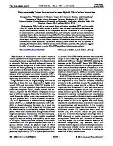
of household members being around 3.8 for both subsamples) (see Table 3) and the difference is significant at 95 percent in both parametric and nonparametric tests. It remains significant as well when we consider the same variable adjusted for the market value of self consumption (significantly larger for affiliated producers) and total income (including other productive activity). From an econometric point of view Becchetti et al. (2008) show that any additional affiliation year raises per capita income from agriculture by a number within the 600-1,200 TBT range. The result remains significant after various robustness checks (propensity score matching, IV estimates with instruments which satisfy exclusion restrictions, estimates on the treatment sample only). Unfortunately we cannot directly use this evidence on productivity gains of affiliated versus non affiliated farmers since we do not have time series but only evidence related to the year of the survey. However, this observed income effect is at the basis of our analysis in which we want to check whether the creation of higher economic value leads farmers to modify their schooling decisions. In Figures 1a and 1b we document the relationship between the likelihood of school enrolment and birth order for affiliated and non affiliated farmers. A first clear cut evidence shows that, on the overall, the probability of going to school is positively correlated with birth order. Such probability starts from 84 percent for the first child and falls up to 71 percent for the fifth child and 53 percent for the sixth child. From a descriptive point of view fair trade affiliation seems to matter for children of lower birth order. The probability of going to school for the fourth child is 80 against 65 percent in affiliated and non affiliated farmer households respectively. The same numbers are 64 and 32 percent when we consider the sixth child. Findings are similar when we look at the probability of going to school (irrespective of the age order) in smaller and larger families. Such probability is roughly the same for affliated and non affiliated single child families while a gap progressively widens as far as the number of children grows and is largest (70 against 32 percent) in families with six children.

16

6. Econometric findings

In the econometric section we want to check whether our descriptive findings are significant and robust when controlling for concurring determinants of child schooling. Based on descriptive evidence showing that affiliation makes a difference when households have more children, we use the number of affiliation years for families with more than two children as regressor measuring the affiliation effect. We then estimate the model in the overall sample (controlling or not for the baseline affiliation year variable) and in the subsample which includes only families with more than two children. The selected specification estimated with logit fixed effects is School ijt   0   1 NChild



l

jt

  2 Trendfutur eFT ijt   3 FTyearl arg efam ijt   4 FTyear ijt 

DYear l   j   ijt

(1)

l

where Schoolijt is a dummy taking value of one if the i-th children of the j-th family went to school in the year t and zero otherwise, Nchildjt is the number of children in the family j at time t, TrendfutureFT is a (pre affiliation) trend variable measuring the number of years in the sample of the child family before entering into FT,16 FTYearlargefam, is the number of FT affiliation years for families with more than two children, FTyear is the number of affiliation years and DYear are time dummies (1989 is the omitted benchmark year). We estimate the selected specification with fixed family effects (ηj). The family effect approach has the disadvantage of hiding the contribution of family time invariant factors (such as parent education) grouping them generically in fixed household characteristics. We will however identify the direction of such effects in the GMM estimate robustness check illustrated in the section which follows.

16

Since all GreenNet farmers are affiliate to Fair Trade after 2001 such variable coincides with the GreenNet affiliation effect before the agreement with fair trade. When evaluated together with FT affiliation years it measures the impact of cooperative membership and organic production, net of the enjoyment of market acces and premium benefits from FT. 17

In the first estimate on the overall sample (Table 4, column 1) affiliation years significantly affect the probability of going to school in households with more than two children. An important element of this finding is that not just the treatment per se, but also the graduation of the treatment (exposure to affiliation) have significant effects on our dependent variable. Controlling for year effects is important here since the latter are obviously correlated with affiliation years. Our result is confirmed when we add to the specification the baseline affiliation year effect which is not significant (Table 4, column 2) and also when we restrict the sample to households with more than two children (Table 4, column 3). In order to eliminate potential heterogeneity between treatment and control sample we reestimate all our specifications in the subsample containing FT affiliated producers only (Table 4, columns 46). The significance of our main variables of interest persists. Consider that, when using this approach we do not have serious problems of heterogeneity between young and old affiliated since the maximum number of affiliation years is relatively small (six) and we have no survivorship bias problems in this relatively short period. Among other variables it worth noting that the pre-affiliation trend (TrendfutureFT) is negative (and strongly significant in three of the six estimates). This is an important indirect check of the validity of the assumption of homogeneity between treatment and control samples. In presence of selection bias and ex ante superior skills of the affiliated producers we should observe a continuity between pre-affiliation and post-affiliation trend effects

on our performance variable (the

probability of sending children to school). This is not the case and, indeed, the negative and sometimes significant effect of affiliation trend indicates a break and not a continuity around the affiliation year. As a robustness check we alternatively estimate the model with a panel probit estimate with random effects. The estimated specification becomes School ijt   0   1 NChild jt   2 Area jt   3 Controlcoo p   4 Birthyear   5Trendfutur eFTijt    6 FTyearl arg efam ijt   7 FTyearijt    l DYearl   j   ijt l

18

(2)

where υj is a normally distributed random family effect. Before estimating the random effect model we check with the Hausman test whether the problem of non orthogonality between regressors and the dependent variable significantly changes estimated coefficient and prevent us from using this approach. We find that the null of no significant difference in coefficients estimated with fixed effects (1) and random effects (2) is rejected in the first two estimates on the overall sample, never rejected when the sample is limited to families with more than two children and around the rejection threshold in the first two estimates with the treatment sample only (columns 4 and 5). What drives the result of the Hausman test is the strong difference in the number of child variable coefficients across the two (random and fixed effect) specifications. If we remove that variable the null is never rejected in all of the six estimates. Consider also that the Mundlak (1978) correction with the introduction of individual averages of relevant regressors across the sample period, which could take partially into account of fixed effects, is not feasible due to serious multicollinearity problems (a VIF far above 10).17The difference between (2) and (1) is therefore the replacement of the fixed with the random effect  jt , with the second approach giving us the possibility of measuring the impact of specific time invariant regressors such as Area (a dummy taking value of one if the producer is located in Kud Chun and zero otherwise), Controlcoop (a dummy for control producers which takes value of one if they belong to a cooperative) and Birthyear (the producer’s year of birth). The reported coefficients measure the change in the probability for an infinitesimal change in each independent, continuous variable and the discrete change in the probability for dummy variables. The significance of affiliation years for families with more than two children is confirmed positive and significant both in the overall and in the FT affiliated only estimates. Under the (probit specific) restrictive assumption of normally distributed link function, the magnitude of the effect indicates

17

The VIF (variance inflation factor) formula is 1/1-R(x) where R(x) is the R squared when the independent variable is regressed on all other independent variables (Marquardt, 1970). If R(x) is low (tends to zero) the VIF test is low (equal to one). A VIF value below 10 (or, more restrictively, five) is considered acceptable by rules of thumb standardly adopted in the literature. 19

that, when affiliation years double with respect to sample mean, the probability of sending children to school raises in a range between 25 and 32 percent according to different estimates. Note as well the strong significance of the year of birth showing that younger producers are more likely to send their children to school. Preformation trends are confirmed as negative also in this estimate.

7. The endogeneity problem

The estimates commented above suffer from two potential endogeneity problems. The first is the selection bias in affiliation. Unobservable factors related with producer’s innate ability and activism can cause both affiliation and the inherited pre-schooling children talents. Together with this we have the traditional endogeneity problem related to the quantity-quality trade-off in the schooling literature. Note that, in principle, we are interested only to the differential effect generated by affiliation on quality for a given level of quantity. Hence, if we assume that the two endogeneity problems are independent from each other, we can focus on the first one (selection bias). Since this assumption may be restrictive, we however adopt a set of strategies which include ways to deal with both biases at a time. More specifically, to address the first problem (which we admit cannot be fully solved) we devise the following three checks. First, we estimate the model in the treatment group only, thereby avoiding distortions related to any sort of heterogeneity between treatment and control individuals (Table 5, columns 4-6).18 Second, we look at preaffiliation trends of affiliated farmers (see the effect of such variable in Tables 5 and 6). A positive preaffiliation trend would create the suspicion that our result is driven by the selection bias since the positive performance in schooling decision by affiliated is already in action before affiliation. We however find negative or insignificant effects 18

Consider that, for a spurious result between affiliation years and child education driven by heterogeneity between young and old affiliated, we should have that old affiliated are more likely to send their children to school. We however control for this and find that the problem does not apply here since there is no significant difference between preformation trends of young and old affiliated. 20

of preaffiliation trends combined with positive and significant effects of affiliation years. Such evidence is in striking contrast with the selection bias. Third, we device in this section a way to tackle both endogeneity problems together. We build a human capital investment index at household level and estimate (at household level) a one step GMM dynamic panel specification where both the number of children in the school age cohort and the number of affiliation years are instrumented by predetermined and exogenous variables. The dependent variable of the household level estimate is a time varying index of human capital investment for each producer, build on retrospective data and represented by the number of children attending school over the total number of children in the schooling age cohort in a given year. More formally, the household schooling investment (HSI) ratio is given by the following expression:

ni

TOTSCH ijt Entryage ijt  Ageijt  Endageijt

j 1

TOTPOTijt Entryageijt  Ageijt  Endageijt

HSI it  

(3)

where the HSIit index is the number of the j children of the i-th producer in a chosen school age cohort (e.g. age range between 619 and 18, if we are interested in elementary, middle and high school, and between 13 and 18 if we are only interested in high school, etc.) who actually went to school in a given year t (TOTSCHijt), divided by the number of children of the i-th producer being in the related school age cohort in the same period (TOTPOTijt).20 In other words, the HSIit index is a ratio of effective to potential household human capital investment. We estimate the model with the following dynamic panel specification HSI( m , l )i,t  0 1 HSI( m , l )i,t 1  2 Schoolyear rsi,t 1 5 FTyeari,t 1  i ,t 1   3 Agei ,t 1   4 Organicyea 6 FTyearlargefami,t 1   k Dtimek   i,t

(3)

k

19

Entry age is generally 5 or 6 and is based on the respondent declaration. The total number of children for each farmer (ni) is indexed to account for heterogeneity in household size. 20

21

where HSI ( m , l ) i ,t is the schooling investment index for the ( m , l ) school age cohort (i.e. from m=6 to l=15 years), Schoolyear and Age are the respondent producer’s schooling years and age respectively, Organicyears are the number of years of organic certification. The other two regressors (FTyear and FTyearlargefam) are the same as in (1). The specification presented in (3) contains lagged values of the dependent variable among regressors. Arellano and Bover (1995) and Blundell and Bond (1998) demonstrate that the correlation between the lagged dependent variable and the error term makes OLS estimates biased and inconsistent, even when error terms are not serially correlated. They develop a GMM approach to tackle this issue. Following them, in the GMM way, we identify a set of endogenous or predetermined, and a set of strictly exogenous, instruments. In the first case we chose the education of the producer and of the producer’s parents. In the second one we chose two and three period lagged values of affiliation years plus year dummies. GMM estimates (as random effects) allow to identify significance of controls which were previously incorporated into fixed effects. As it is obvious to believe, the strong significance of the lagged dependent variable confirms that the household schooling investment index is strongly autocorrelated. Beyond persistence, the dependent variable is positively affected by parental (father) education, consistently with standard results in the literature (Edmonds, 2007), while household respondent age is not significant (Table 6). The effect of preaffiliation (negative) and affiliation (positive) years in our GMM estimate at household level is consistent with what found in fixed family effect estimates at individual child level (Tables 4 and 5). The test on the residual autocorrelation structure does not reject the hypothesis of second (while not first) order autocorrelation. The Hansen test on overidentifying restrictions is robust and not unreasonably high. This reflect the parsimonious use of instruments we made in the estimates by using only second and third lag for GMM instruments.

22

Note that the null of exogeneity of our instrumented variables is not rejected by the DavidsonMcKinnon test but only if we consider the 1 percent significant threshold. As a robustness check, following what found in the child unit estimates presented in Tables 4 and 5, we modify the specification by adding the baseline affiliation year effect among regressors (Table 6, column 2). The exogeneity test is not passed in this case. When we restrict the sample to treatment producers only our main result holds (Table 6, column 3) and the exogeneity is closer to the rejection of the null (and definitely so in the specification in which we add the baseline affiliation year effect among regressors (Table 6, column 4)).

8. Conclusions

Poverty can be usefully conceived as a set of exclusions (from credit, product markets, insurance, education) which prevent individuals from fully exploiting their talents, limiting their productive contribution to the society. In this paper we demonstrate how exclusions can interact with each other generating virtuous or vicious circles. More specifically, by performing an impact study on the effects of affiliation to fair trade for a cooperative of organic farmers, we document that the improvement of access to foreign markets (with a package of initiatives promoted by FT) has positive and significant effects on access to education of children when producers have large families. Our findings document that years of affiliation significantly ease the well known quantity/quality trade off (which also implies a lower probability of school enrolment for children in larger families). From a methodological point of view we obtain these results by developing a retrospective panel data approach based on memorable events and control for selection bias and endogeneity with various techniques (analysis of preformation trends, restriction of the estimate to the treatment sample only, adoption of GMM estimates to cope with endogeneity).

23

Our findings are consistent with FT criteria and prediction from the luxury axiom. A plausible interpretation consistent with observed FT criteria and characteristics is that FT affiliation raises producers revenue by easing access to foreign markets and financing technical innovation. This enables producer families to overcome those income thresholds which induce them to send more their children to school when families are large.

References Arellano, M., and O. Bover, (1995); Another look at the instrumental variables estimation of error components models. Journal of Econometrics 68: 29-51 Bacon, C. (2005). Confronting the Coffee Crisis: Can Fair Trade, Organic, and Specialty CoffeesReduce Small-Scale Farmer Vulnerability in Northern Nicaragua? World Development 33(3), 497-511. Baland, J.M. and Duprez, C. (2008); Are Fair Trade Labels Effective Against Child Labour? CEPR Discussion Paper No 6259. Basu K. and Van P.H., (1998); The Economics of Child Labor. American Economic Review 88:412-427. Basu, K. and Van, P.H. (1998), ‘The Economics of Child Labor’, American Economic Review 88(3): 412-27. Becchetti L., Castriota S., Michetti M., (2008); Testing the luxury axiom: the effects of fair trade on child schooling decision on a sample of Chilean honey producers, mimeo. Becchetti L., Conzo P. and Gianfreda G., (2009). Market access, organic farming and productivity: the determinants of creation of economic value on a sample of fair trade affiliated Thai farmers. Econometica Working Papers wp05, Econometica. Becchetti, L. Giallonardo E. Tessitore, N. (2008); Ethical product differentiation with symmetric costs of ethical distance. Rivista di Politica Economica, forth. Becchetti L., Costantino M. (2008); Fair trade on marginalized producers: an impact analysis on Kenyan farmers. World Development 365: 823–842. Becchetti L., Michetti, M., (2008); When Consumption Generates Social Capital: Creating Room for Manoeuvre for Pro-Poor Policies. Ecineq working papers 88. Becchetti L., Solferino, N. (2008). On ethical product differentiation, Economia e Politica Industriale, (forth).

24

Becchetti L., Rosati F. (2007); Globalisation and the death of distance in social preferences and inequity aversion: empirical evidence from a pilot study on fair trade consumers, The World Economy, 30 (5): 807-30. Becchetti L. Costantino M. Portale E., 2007, Human capital, externalities and tourism: three unexplored sides of the impact of FT affiliation on primary producers, CEIS working paper n. 262 Becker, Gary S., and Nigel Tomes, (1976). “Child Endowments and the Quantity and Quality of Children,” Journal of Political Economy, 84(4) Part 2, S143-S162. Bhalotra, S., Heady, C. (2003); Child Farm Labor: The Wealth Paradox. World Bank Economic Review 17(2): 197-227. Black, S. E., Devereux P. J. and Salvanes K. G. (2005); The More the Merrier? The Effect of Family Size and Birth Order on Children’s Education. Quarterly Journal of Economics, 120(2), May. Blundell, R., Bond S. (1998); Initial conditions and moment restrictions in dynamic panel data models. Journal of Econometrics 87: 11,143. Booth, A. L. and Kee, H. J. (2009); Birth Order Matters: The Effect of Family Size and Birth Order on Educational Attainment. Journal of Population Economics, April 2009, v. 22, n. 2, pp. 367-97. Castro, J.E. (2001); Impact assessment of Oxfam's fair trade activities. The case of Productores de miel Flor de Campanilla. Oxford: Oxfam. Cigno, A., Rosati, F. (2005). The Economics of Child Labour. (Oxford University Press, Cambridge). Cigno, A., Rosati, F. and Z. Tzannatos (2002), Child Labor Handbook. WB Social Protection Discussion Paper N. 0206. Davidson, R. and MacKinnon, J. (1993); Estimation and Inference in Econometrics. New York: Oxford University Press. Deb, P. and Rosati, F. (2002); Determinants of Child Labor and School Attendance: The Role of Household Unobservables. Understanding Childrens Work Working Paper. Florence: Innocenti Research Center. Edmonds, E. V., (2007); Child labor. NBER Working Paper n. 12926 Ejrnaes M. and Portner C. C. (2004); Birth Order and the Intrahousehold Allocation of Time and Education. Review of Economics and Statistics. LXXXVI(4), Nov. 1008-19. Guarcello L., Mealli F., Rosati F. (2002). Household Vulnerability and Child Labour: the Effect of Shocks, Credit Rationing and Insurance. UCW Working Paper 3, Understanding Children's Work (UCW Project). Hanushek, E. A. (1992); The Trade-off between Child Quantity and Quality. Journal of Political Economy, Vol. 100, No. 1. (Feb., 1992), pp. 84-117.

25

Hayes, M. (2004); Strategic management .

implication

of

the

ethical

consumer.

Iacovou, M. (2001); Family Composition and Children's Educational Outcomes. Working Paper of Institute for Social and Economic Research, paper 2001-12 (PDF). Colchester: University of Essex. (June). Kohler P. (2007); The Economics of Fair Trade: For Whose Benefit? An Investigation into the Limits of Fair Trade as a Development Tool and the Risk of Clean-Washing.06-2007, HEI Working Papers. LeClair, M. S. (2002); Fighting the tide: Alternative trade organizations in the era of global free trade. World Development 30(7): 1099–1122. Marquardt, D. W. (1970). Generalized inverses, ridge regression, biased linear estimation, and nonlinear estimation, Technometrics 12,591–612. Maseland, R., & De Vaal, A. (2002); How Fair is Fair Trade? De Economist 150(3): 251-272. McIntosh, C., Villaran, G. and Wydick, B. (2007); Microfinance and Home Improvement: Using Retrospective Panel Data to Measure Program Effects on Fundamental Events. University of San Francisco Departmental Working Paper. Moore, G. (2004); The Fair Trade Movement: parameters, issues and future research. Journal of Business Ethics 53(1-2): 73-86 Mundlak, Y. (1978). On the Pooling of Time Series and Cross Section Data. Econometrica, 46 (1), 69–85. Nelson, V. & Galvez, M. (2000); Social Impact of Ethical and Conventional Cocoa Trading on Forest-Dependent People in Ecuador. University of Greenwich. Pariente, W. (2000); The impact of fair trade on a coffee cooperative in Costa Rica. A producers behaviour approach. Université Paris I Panthéon Sorbonne, No 1161-98, University of Wisconsin. Psacharopoulos G., Patrinos H. (1995); Educational Performance and Child Labor in Paraguay. International Journal of Educational Development, 15(1): 47-60. Psacharopoulos G. (1997); Child Labor Versus Educational Attainment: Some Evidence from Latin America. Journal of Population Economics, 10(4): 377-386. Ranjan, P. (2001), Credit Constraints and the Phenomenon of Child Labor. Journal of Development Economics, LXIV, 81-102. Redfern, A. & Snedker, P. (2002); Creating market opportunities for small enterprises: experiences of the fair trade movement. ILO, Geneva. Reinstein, D. and J., Song (2008); Efficient Consumer Altruism and Fair Trade. Economics Discussion Papers 651, University of Essex, Department of Economics.

26

Ronchi, L. (2006); "Fairtrade" and Market Failures in Agricultural Commodity Markets. World Bank Policy Research Working Paper 4011. Washington: IBRD. Ronchi, L. (2002); The impact of fair trade on producers and their organizations: a case study with Coocafè in Costa Rica. University of Sussex. Ruben, R., (2008); The impact of fair trade. Wageningen Academic Publishers, Wageningen. Steelman, L. C., and Powell, B. (1989); Acquiring capital for college: The constraints of family configuration. American Sociological Review, 54, 844–855. Yilmazer, T. (2008); Saving for Children’s College Education: An Empirical Analysis of the Tradeoff Between the Quality and Quantity of Children, Journal of Family Economic Issue, 29, n. 2, 307324.

27

Table 1 Price formation in Bak Reua and Kud Chun cooperatives Bak Reua October 2007 - organic farmers discussed about the price of the paddy and set it around: January 2008 – Conventional farmers received from the market the same price as organic farmers (THB 10000). Organic farmers hence asked GreenNet to receive a higher price as incentive for remaining affiliated. Finally GreenNet increased the price for organic paddy of: Hence, for organic farmers the guaranteed price for 2008 is on average: Additionally, the FT premium that goes only to producer’s group is for 2008 (according to FLO law): The FT bonus (also called paddy fund) that goes directly to organic farmers is: Further FT benefits: Local cooperative dividend (to organic and conventional members).

Fair-trade premium utilization

Kud Chun THB 10,000

+ THB 2,500

= THB 12,500 [Paddy price can still vary according to quality]. + THB 750

+ THB 1,280 Local training, extension activities, advising and support to organic farmers Variable (positive) computed as follows: Variable 8% of the capital share farmers (0 in the last years) invested in the cooperative + THB 50 per ton of paddy sold. The premium is divided into (a) 50% is allocated to the mill to several funds to which farmer improve its management members can apply for support (b) 25% is allocated to the (a) green manure seed extension works (b) farmer training (c) 25% is allocated for Organic (c) member welfare, e.g. Fair-Trade Fund. This Fund has education of their children, also contribution from other natural disaster relief sources and provides loans to members who wish to convert to sustainable production as well as other community benefits.

Local cooperative funds (to organic and conventional members) taken from cooperative profits.

Loans Saving Groups

28

Table 2. Summary information on the samples THE “TREATMENT” GROUP AND THE “CONTROL GROUP IN THE WHOLE AREA Number of Observations

360

N. of fair trade affiliated organic farmers (treatment group)

180

N. of non fair trade affiliated non-organic farmers (control group)

180

Total n. of farmers affiliated to cooperatives

288

N. of control group farmers non affiliated to cooperatives

72

N. of control group farmers affiliated to cooperatives

108

N. of Farmers in conversion

14 BAK REUA

Number of Observations

210

N. of fair trade affiliated organic farmers (treatment group)

105

N. of non fair trade affiliated non-organic farmers (control group)

105

Total n. of farmers affiliated to cooperatives

162

N. of control group farmers non affiliated to cooperatives

48

N. of control group farmers affiliated to cooperatives

57

N. of Farmers in conversion

7 KUD CHUM

Number of Observations

150

N. of fair trade affiliated organic farmers (treatment group)

75

N. of non fair trade affiliated non-organic farmers (control group)

75

Total n. of farmers affiliated to cooperatives

126

N. of control group farmers non affiliated to cooperatives

24

N. of control group farmers affiliated to cooperatives

51

N. of Farmers in conversion

7

29

Table 3. Confidence intervals of selected variables for FT producers and the control sample Variables Socio-demographic features Ft years Certification years Age School years People in the household Number of children

Ft producers [95% Conf. Interv.]

Obs.

Mean

180 180 180 180 180 180

5.283*

5.078092 5.488574

6.888* 49.1 6.611* 3.827 2.488

Income, productivity and investment Income from agriculture Total income Family income Temporary employees Employee daily wage Land size Total productivity Productivity of the 1st working activity Productivity of the 2nd working activity Investment in input Price, sales and trading conditions

180 180 180 180 86 180 180 180 92 180

Local (non GreenNet) cooperative price FT price

Non Ft producers [95% Conf. Interv.]

Obs.

Mean

6.431667 7.34611 47.41761 50.78239 6.132579 7.089643 3.613573 4.041983 2.302008 2.675769

180 180 180 180 180 180

0 0 51.32222 5.905556* 3.766667 2.55

49.51545 53.129 5.49255 6.318561 3.516413 4.01692 2.331082 2.768918

60942.49* 78778.61* 104897.3 3.822* 156.279 26.080 93.749* 125.891 49.014* 14651.67

55225.46 70469.44 92479.45 2.914331 147.1056 24.17416 77.02672 104.4428 32.77152 2960.193

66659.53 87087.77 117315.2 4.730113 165.4525 27.98695 110.4715 147.3399 65.25622 26343.14

179 179 179 180 69 180 177 177 85 180

41646.37* 55173.74* 87089.39 2.55* 153.7681 23.85556 67.43628* 98.40271 25.87522* 5265.556

36363.51 48040.08 72814.02 1.87567 148.6373 21.61981 54.95465 72.09847 19.59875 258.4469

46929.22 62307.41 101364.8 3.22433 158.899 26.0913 79.91791 124.7069 32.15169 10272.66

177

11305.73*

11141.69

11469.76

81

10019.32*

9824.894

10213.75

177

13940.98

13832.28

14049.68

Other buyers price

4

11583.25

4267.535

18898.96

116

10420.78

9916.863

10924.69

Cooperatives advance payments

176

.0454545

.0143782

.0765309

176

0

GreenNet dividends

177

306.0904 *

219.1588

393.022

77

101.2597*

56.44248

146.077

Other cooperative dividends

6

14

-7.197561

35.19756

115

40.6087

7.949534

73.26786

Household weekly food expenditure

180

430.7111

381.1277 480.2945

180

461.5556

419.4204

503.6907

Rice self-consumption share

180

100

100

180

100

100

Noodles self-consumption share

170

.2941176

-.2865001

167

1.197605

-.4693058

Vegetables self-consumption share

180

81.33333*

77.6292

180

71.30556*

66.74405

75.86706

Papaya self-consumption share

180

79.35*

74.34501

84.35499

179

67.7933*

61.65727

73.92932

Fresh fruit self-consumption share

180

53.96111*

48.87574

59.04649

180

39.55556*

34.51099

44.60012

Food expenditure and self-consumption 100 .8747354 85.03747

100 2.864515

Eggs self-consumption share

180

25.98889*

19.91602

32.06176

179

16.98324*

11.77462

22.19186

Milk self-consumption share

170

3.582353

.7799004

6.384805

170

2.411765

.1084575

4.715072

45.86483

59.86551

56.10313

Chicken self-consumption share

178

52.86517

Other meat self-consumption share

177

0 75.70292

179

49.27374

42.44436

177

.0564972

-.0550019

179

57.15084*

51.09267

63.209

175

.5714286

-.5563951

1.699252

.1679963

Fish self-consumption share

180

70.38889*

65.07485

Fresh noodles self-consumption share

172

.5813953

-.5662407

Market value of self consumption

180

29502.66*

27029.26

31976.06

180

24216.51*

21754.81

Debt/income

180

1.040396

.7944135

1.286379

179

1.24762

.9143597

1.58088

Saving/income (percent)

180

15.56389*

12.96199

18.16578

180

11.46944*

9.378305

13.56058

Number of durables owned

180

8.333333 *

8.144836

8.521831

180

7.5*

7.258395

7.741605

1.729031

26678.21

Savings, debt and wealth

5 percent significance of the difference in means between affiliated and non affiliated farmers. Source Becchetti, Conzo and Gianfreda (2008)

30

Figure 1a Schooling probability and birth order. Legend. Vertical axis: probability of going to school, horizontal axis birth order in the family. Control group (dashed line); FT affiliated (continuous line). 1 0.9 0.8 0.7 0.6 0.5 0.4 0.3 0.2 0.1 0 n_children 1

n_children 2

n_children 3

n_children 4

n_children 5

n_children 6

Child horder

Figure 1b Schooling probability and number of children in the family. Legend. Vertical axis: probability of going to school, horizontal axis number of children in the family. Control group (dashed line); FT affiliated (continuous line). 1 0.9 0.8 0.7 0.6 0.5 0.4 0.3 0.2 0.1 0 children 1 children 2 children 3 children 4 children 5 children 6

31

Table 4. The effect of Fair Trade affiliation on schooling decisions: conditional fixed effect logistic regression All sample Treatment sample only Families with more than two children only

Families with more than two children only Sons Trendsaraflo Ftagehighc

-1.024 (-1.56) -0.001 (-2.22) 0.702 (4.51)

FT Age Year dummies

Yes

-1.025 (-1.56) -0.002 (-1.74) 0.695 (4.31) 0.0283 (0.17) Yes

N. of Obs. 3464 3464 Nr. of Groups 181 181 LR χ2 (22) 495.60 495.63 Log Likelihood -1131.699 -1131.685 Prob > χ2 0.000 0.000

-1.120 (-1.40) -0.001 (-1.73) 0.764 (1.67)

Yes

-1.488 (-1.88) -0.001 (-2.83) 0.676 (4.22) 0.247 (1.11) Yes

2156 115 347.67 -684.689 0.000

2156 115 348.97 -684.043 0.000

1038 47 48.62 -415.995 0.001

-0.774 (-1.24) -0.001 (-1.28) 0.604 (1.93)

-1.481 (-1.88) -0.001 (-3.10) 0.715 (4.53)

Yes 1861 82 87.84 -740.322 0.000

Yes

The estimated specification is

School ijt   0   1 NChild

jt

  2 Trendfutur eFTijt   3 FTyearl arg efam ijt   4 FTyearijt  (1)

   l DYearl   j   ijt l

where Schoolijt is a dummy taking value of one if the i-th children of the j-th family went to school in the year t and zero otherwise, Nchildjt is the number of children in the family j at time t, TrendfutureFT is a (pre-formation) trend variable measuring the number of years in the sample of the child family before entering into FT, FTYearlargefam, is the number of FT affiliation years for farmilies with more than two children, FTyear is the number of affiliation years, DYear are time dummies (1989 is the omitted benchmark year) and ηj are fixed family effects.

32

Table 5. The effect of Fair Trade affiliation on schooling decisions: random effect probit regression (marginal effects) All sample

Sons Area Controlcoop Agriculture Birthyear Trendsaraflo

-0.138 (-2.23) -0.881 (-5.58) 0.0361 (0.17) -0.016 (-1.78) 0.1038511 (8.62) -0.0001 (-1.12)

Year dummies Cons

Hausman test* (p-value) N Nr. of Groups LR χ2 (26) Log Likelihood Prob > χ2

Families with more than two children only -0.208 (-2.21) -0.191 (-0.82) 0.190 (0.34) 0.003 (0.29) 0.003 (5.87) -0.001 (-0.67)

-0.0236 (-2.26) 0.094 (6.55) -0.001 (-2.00)

0.254 (1.83) Yes -194.408 (-5.75)

0.309 (4.42) Yes -199.660 (-8.39)

-0.136 (-2.19) -0.883 (-5.60) 0.208 (0.64) -0.0158 (-1.79) 0.104 (8.63) -0.001 (-1.25) 0.050 (0.71) 0.303 (4.29) Yes -200.397 (-8.40)

(0.00)

(0.00)

(0.56)

(0.02)

(0.05)

(0.99)

5652 325 461.18 -1760.423 0.0000

5652 325 459.89 -1760.169 0.0000

2820 137 110.03 -1045.842 0.0000

3870 228 367.20 -1088.801 0.0000

3870 228 368.92 -1087.628 0.0000

1798 89 99.51 -595.019 0.0000

Ftage Ftagehighc

Treatment sample only Families with more than two children only -0.334 -0.272 -0.2689 (-3.47) (-3.38) (-3.32) -0.531 -1.239 -1.244 (-1.77) (-6.35) (-6.40)

-0.006 (-0.40) 0.102 (5.45) -0.001 (-1.38)

0.324 (4.57) Yes -179.341 (-6.33)

-0.024 (-2.27) 0.094 (6.59) -0.001 (-2.34) 0.141 (1.51) 0.313 (4.39) Yes -180.752 (-6.39)

0.318 (1.65) Yes -196.656 (-5.34)

The estimated specification is School ijt   0   1 NChild

jt

  2 Area jt   3 Controlcoo p   4 Birthyear   5Trendfutur eFTijt 

  6 FTyearl arg efam ijt   7 FTyearijt    l DYearl   jt   ijt

(2)

l

where Schoolijt is a dummy taking value of one if the i-th children of the j-th family went to school in the year t and zero otherwise, Nchildjt is the number of children in the family j at time t, Area is a dummy taking value of one if the producer is located in Kud Chun and zero otherwise, Controlcoop is a dummy for control producers which takes value of one if they belong to a cooperative, Birthyear is the producer’s year of birth), TrendfutureFT is a (pre-formation) trend variable measuring the number of years in the sample of the child family before entering into FT, FTYearlargefam, is the number of FT affiliation years for farmilies with more than two children, FTyear is the number of affiliation years, DYear are time dummies (1989 is the omitted benchmark year) and  jt are random effects. Hausman test. H0: the coefficients of the random (this Table) and the fixed effect estimate (Table 4) are not significantly different from each other.

33

Table 6. Robustness check: GMM estimates on the effects of FT affiliation on the Household Schooling Index (HSI) ALL SAMPLE HSIt-1

0.840 (12.74) 0.046 (2.75) -0.005 (-1.38) -0.016 (-2.33)

Schoolyear Age Organicyears

0.854 (11.48) 0.016 (1.07) -0.003 (-0.81) -0.011 (-1.78)

0.038 (2.55) 0.126 (0.60) 2567

0.829 (11.73) 0.044 (2.58) -0.005 (-1.45) -0.019 (-2.37) 0.019 (0.35) 0.033 (1.62) -0.310 (-1.12) 2567

0.041 (4.06) 0.172 (0.94) 1566

0.841 (10.95) 0.017 (1.08) -0.003 (-0.89) -0.016 (-2.52) 0.137 (1.12) 0.034 (2.93) 0.191 (1.03) 1566

266

266

165

165

-7.79

-7.75

-6.45

-6.37

(0.000)

(0.000)

(0.000)

(0.000)

-0.73

-0.75

0.68

0.66

(0.466)

(0.455)

(0.498)

(0.510)

89.24

89.91

108.67

107.34

(0.082)

(0.064)

(0.002)

(0.002)

55.21

53.38

56.21

56.79

(0.929)

(0.941)

(0.884)

(0.853)

3.334

7.825

2.963

0.807

0.019

0.001

0.031

0.490

Ftage Ftagehighc Cons Number of obs. Number of groups AR(1) test Prob> χ2 AR(2) test Prob> χ2 Sargan test Prob> χ2 Hansen test Prob>chi2 Davidson-McKinnon exogeneity test P-value

TREATMENT GROUP ONLY

The base specification is:

HSI ( k , l ) i ,t   0   1 HSI ( k , l ) i ,t 1   2 Schoolyear

  5 FTyearl arg efam i ,t 1    k Dtime k   i ,t

i , t 1

  3 Age i ,t 1   4 FTyear i ,t 1 (3)

k

where HSI ( k , l ) i ,t is the schooling investment index for the ( k , l ) school age cohort, Age and Schoolyear are the respondent producer’s age and schooling years respectively, Organicyears are the number of years of organic certification, Dtime are year dummies, FTyearlargefam, is the number of FT affiliation years for farmilies with more than two children and FTyear is the number of affiliation years. The equation is estimated with a system GMM model with two-step coefficients and Windmejier (2005) correction to obtain unbiased standard errors. Variables used for building endogenous or predetermined (GMM) instruments are producer’s and producer’s mother and father schoolyears. Variables used for building strictly exogenous instruments are two and three period lagged affiliation years. Time dummy coefficients are omitted and available upon request. The Sargan and Hansen statistics are distributed as a χ2 under the null of instrument validity. AR(1) and AR(2) are tests for first and second order serial correlation in the residuals, asymptotically distributed as a N(0,1) under the null of instrument validity. The DavidsonMcKinnon statistic is distributed as an F under the null of orthogonality of the set of strictly exogenous instruments to the error term of the base estimate. * We estimate the model in the subsample of the control group and the treatment group before affiliation. We introduce a variable in which a linear trend is multiplied for the treatment group dummy and test whether the latter it is significantly different from zero. The table reports the coefficient and the t-statistics.

34

Appendix 1 Variable legend Variables Area 1

Description Variable taking value of 1 if respondents live in Kud Chun Variable taking value of 1 if respondents live in Bak Reua Dummy taking the value of 1 if respondents are affiliated to FT and 0 otherwise Respondents’ Age

Variables Employee daily wage

Description Temporary employees’ daily wage

Investment in input

Investment in input during last year

Male

Dummy taking the value of 1 if respondents are male

Married

Dummy taking the value of 1 if respondents are members of cooperatives buy are not FT affiliated Years of school attendance

Divorced

Dummy taking the value of 1 if respondents are married Dummy taking the value of 1 if respondents are divorced

Certification years Certification years 1

Family food consumption Rice Noodles Vegetables Papaya Fresh fruit

Number of children Number of people living in the household Household’s food expenditure in a week % of rice self-produced % of noodles self-produced % of vegetables self-produced % of papaya self-produced % of fresh fruit self-produced

Egg Milk

% of eggs self-produced % of milk self-produced

FT price Ft premium

Chicken

% of chicken self-produced

Other buyers price

Other meat

% of other meat self-produced

Cooperatives advance payments

Fish

% of fish self-produced

Cooperatives profit/dividends

Area 2 Affiliation dummy Age Control group School years Number of children People in the household

Unmarried

Certification years 2 FT years FT years 1 FT years 2 Durables owned Cooperatives price

Fresh noodles

% of fresh noodles self-produced

Other buyers profit/dividends

Value of self consumption (per year) Years in agriculture

Value of self-production (per year) Working years in agriculture

Total productivity Productivity 1st activity

Income from agriculture

Respondents’ yearly income in agriculture Respondents’ yearly income from the main and the second activity The sum of the yearly income earned by all members of the household Number of the respondents’ temporary employees Exogenous events having a positive impact on respondents’ income i) increase in the paddy rice market price, ii) a positive shock on production, iii) present from farmers’ sons and daughters (money or, in same cases, a car), v) wage shock in the second activity, vi) lottery winning and vii) granting of awards.)

Productivity 2nd activity

Total income Family income Temporary employees Positive exogenous events

Distance from cooperatives

Distance from cooperatives

35

Debt/income Saving/income Land size Negative exogenous events

Dummy taking the value of 1 if respondents are unmarried Number of organic certification years Certification years in area 1 (Kud Chun) Certification years in area 1 (Bak Reua) Number of FT affiliation years FT years in area 1 (Kud Chun) FT years in area 1 (Bak Reua) Sum of durables owned by respondents Price of Jasmine rice paid by local cooperatives Fair trade price for Jasmine price Difference betweem FT price and the price payed by local cooperatives Price of Jasmine rice paid by other buyers Advance payment from local cooperatives (Jasmine rice) Profit/dividend received from local cooperatives (Jasmine rice) Profit/dividend received from other buyers (Jasmine rice) Total income per hour worked Respondents’ income from agriculture per hour worked Respondents’ income from second activity per hour worked Family debt to income ratio Last year saving as a percentage of income Total land size (rai) Exogenous events having a negative impact on respondents’ income (i) close relatives’s death, ii) desease, iii) car accidents, iv) fire, v) car breaking, an vi) increase in the input market price, vii) the death of animals used as capital investment (such as water buffalos), viii) a slow development of the soil.)

Appendix 2 Questionnaire N° Question Alternatives 1 Case number CG or TG 2 Sex female [1] male [3] 3 Age number 4 Civil status Unmarried [1] divorced [3] married [5] Are you member of a 5 cooperative/producers' yes [1] group? no [0] If 5 = yes: How far do you 6 live from the cooperative km center (in Yasothon)? How many people in your 7 household migrated in the number last five years? Relatives moved as 8 If 7 = yes: What for? well [1] Schooling [3] Marriage [5] Look for work/start new job [7] Famine, draught, disease [9] Other (specify)________[11 ] 9 if 7 = yes: Where? Other village [1] Bangkok [3] Other-Non-Bangkok [5] Other-non-Thailand [7] How much do you 10 consider yourself happy 0-10 (from 0 to 10)? How many years have you 11 years attended the school? How many children do you 12 number have? [fill the tab below] 13 Children tab Sex

Male [1] Female [3]

Activity

Age

How old when started the school?

First Second Third Fourth Fifth Sixth Seventh Eighth How far do you live from 14 km the school? During the last year your children went to school 15 baht how much have you spent on education for? Fees Uniforms Textbooks

36

How many years did he/she attend the school?

How many years did he/she help the repeat? [if family [1] not = 0]

work outside not the working family [5] [3]

how many hours/da y does he/she work on that activity?

Exercise books, pens, pencils Meals, transportation Other expenses Where was your last child 16 at home [1] born? in a rural clinic [3] in the hospital [5] other (specify) [7] Has your last child been 17 yes [1] vacccinated? no [0] How much did you spend 18 this year for dental care for baht the whole family? Has one of your children number of children 19 died? died Have you seriously injured 20 yourself during the last how many times year? How many days have you 21 got sick and could not go days to work? If you were to sell your 22 plot of land today, how baht/RAI much could you sell it for? Do you use any chemical 23 yes [1] fertilizer/pesticide? no [0] If 23 = no: Did you use 24 chemical ferilizer/pesticide yes [1] in the past? no [0] if 24= yes: When did you 25 year stop using them? How many people do 26 number usually live in your house? During the past year, how many times have you times [0 if not 27 attended extension training attended] activities? If 27>0: What kind of 28 Use of fertilizers [1] training courses? Irrigation [3] New seeds [5] Pest infestation [7] Blight problems [9] soil problems [11] weather problems [13] general crop advice [15] marketing advice [17] insemination services [19] other (specify) _______ [21] 29 If 27=0: Why? I am not interested [1] I don't have time [3] I can't afford them [5] there aren't training courses [7] Which is the main building 30 material used for your timbers [1] house? bricks and concrete [3] other [5] Which kind of floor is 31 bare ground [1] there in the house?

37

cement [3] wood boards [5] tiles [7] other [9] 32

33

34 35

36

Which is the main light electricity [1] source you have at home? gas [3] oil lamp [5] candle [7] other (specify) [9] What type of fuel does your family mainly use for wood [1] cooking? coal [3] gas [5] electricity [7] dung [9] other (specify)________ [11] Has your family access to yes [1] drinkable water? no [0] Bathroom location and inside and exclusive sharing: [9] inside and shared [7] outside and exclusive [5] outside and shared [3] no bathroom [1] How much do usually you spend in food for all your bath family in a week?

37 Consumption TAB

How many times does your family eat the following food?

every day [1]

twice a week once a once a never [9] [3] week [5] month [7]

Rice Noodles Vegetables Green Papaya Fresh fruit Eggs Milk Chicken Other meat Fish Fresh noodles How do you consider your standard of living 38 compared to the one of much better [1] other people who live in this village? better [3] equal [5] lower [7] much lower [9] Besides agriculture do you 39 craftwork [1] have another activity? construction [3] other (speficy)_____ [5] 40 Activities' Tab

Years

Earnings/yea Days Hours r worked/Y worked/day

38

Which share of each food consumed do you produce by yourself? 0 - 100 %

ear Agricolture Second How many employees do 41 Number of employees Daily wage you have? stable employees temporary employees Are you usually involved 42 in a labour exchange yes [1] system? no [0] Which share of Buyers Tab - Who do you production do you 43 usually sell Jasmine Rice usually sell to each to? type of buyer?

%

44

45

46

47

48

49

Which price do you usually receive per ton sold? baht/ton

How much did you Do you receive as receive profit/divid How much are you satisfied with the money in end from price? advance? the producer's group? Yes [1] [1= very much 2= enough; 3= not very baht satisfied; 4= not at all] No [0]

Local cooperative Other buyers During last five years have you changed your yes [1] production system? no [0] Please tell me the yearly baht income in your family. husband/wife sons/daughters other members Do you have other sources of non work income yes [1] (subsidies, donations, etc.) ? from the community no [0] from the state from private persons from development agencies/ngos remittances from relatives rents other (specify)_____ Which of the following things does your family yes [1] no [0] own? tv entertainment devices (CD, DVD players, etc.) fridge bicycle motorcycle car water pump plowing machine gas stove truck mobile phone How much are you satisfied with your [0 - 10] household’s living conditions? How much do you consider yourself a good [0 - 10] farmer?

39

40