Statement of Problem. The problem of visibility ... 1.2. Visibility Information. In order to optimize visibility information, one must first be able to calculate .... In the case where x is on the zero level set of Ï(·;x0 +ε), this reduces to. âK|ε| ⤠Ï(x;x0) ...
VISIBILITY OPTIMIZATION USING VARIATIONAL APPROACHES LI-TIEN CHENG AND YEN-HSI TSAI A BSTRACT. Constructing the visible and invisible regions of an observer due to the presence of obstacles in the environment has played a central role in many applications. It can also be a first step. In this paper, we adopt a visibility algorithm that can produce a variety of general information to handle the optimization of visibility information. Through the use of level set tools, gradient flow, finite differencing, and solvers for ordinary differential equations, we introduce a set of distinct algorithms for several model problems involving the optimization of visibility information.
1. I NTRODUCTION 1.1. Statement of Problem. The problem of visibility involves the determination of regions in space visible to a given observer when obstacles to sight are present. When the observer is replaced by a light source in the simplified geometrical optics setting with perfectly absorbing boundary condition at the obstacles, the problem translates to that of finding illuminated regions. In this paper, we consider a class of optimization problems associated with visibility and solve them through application of the approach introduced in [12] which, though replaceable, provides enough information to handle each of the problems. Let D be the set of points comprising one or several given solids in a compact subset Ω of Rd . A solid here refers to an opaque obstruction. We seek solutions to three central questions involving visibility optimization. The first question is: • What is the optimal location x0 for an observer such that the volume of the visible region in Ω is maximized? A larger class of problems emerges when variations and extensions involving the observer and the space – multiple observers, moving observers, optimality under different measures – are taken into account. Therefore, our second question adds to the first: • What are the optimal locations {xi } for a collection of observers, so that jointly the volume of the visible region in Ω is maximized? Lastly, we ask: • What is the optimal path γ(t) of an observer, traveling from A to B, so that the volume of the visible region in Ω is maximized? One can interpret the last question as an extension of the second with an uncountable number of observers distributed along the path. Problems related to the three questions above can be found in applications dealing with geometric optics, scattering, path planning, digital surface reconstruction, photolithography, and dynamic games, to name a few (see, e.g., [1, 2, 3, 6, 7]). In many situations, it is useful to think of the observer as a light source. Consequently, our attempt to solve the three central questions amounts to maximizing the illuminated regions in Ω, or the average illumination (exposure) in Ω. The core of this work revolves around adaptivity in observer locations and optimization related to the corresponding visibility. Thus, it does not detract from the essence of our study to disregard global optimality and accept local maxima as suitable solutions, with gradient flow a valid process. 1.2. Visibility Information. In order to optimize visibility information, one must first be able to calculate that information. A plethora of options are available, most arising from computational geometry and some 1
VISIBILITY OPTIMIZATION USING VARIATIONAL APPROACHES
2
1
0.8
0.6
0.5
0.4 0
0.2
0 −0.5
−0.2
−0.4 −1 1
−0.6
1
0.5 0.5
0
−0.8
0 −0.5
−1 −1
−0.8
−0.6
−0.4
−0.2
0
0.2
0.4
0.6
0.8
−0.5 −1
1
−1
F IGURE 1.1. For the obstacle environment and given observer location of plot on the left, the visibility level set function is shown in the plot on the right. from partial differential equations. For a chosen application, certain ones may be preferable; for example, a user may be interested only in a limited amount of visibility information, or have hardware constraints, or emphasize speed over accuracy, or vice versa. Since we are not concentrating on a specific application, we seek one that provides sufficient information that allows for accurate numerical differentiation and integration in the whole space. This may be non-optimal for some specialized graphics applications but will allow us to use the same algorithm independent of application and especially in situations outside of the usual context of computer graphics and vision. Other approaches can be substituted when specific applications are of interest. Thus, we choose to use the algorithm introduced in [12] to generate our visibility information. This algorithm works with an implicit representation of obstacle surfaces and generates an implicit description of the visibility information with a PDE-based method (see Figure 1.1). The advantage is, as mentioned above, in the substantial amount of information that can be extracted from this description. Under simple operations, one can obtain accurate location of shadow boundaries, including their normal vectors, curvatures, surface areas, and even the distance of points away from them; accurate location of visible and invisible regions, including their volumes; and a partial differential equation viewpoint for analysis. The disadvantage is in the inefficiency of the approach in typical computer graphics applications such as rendering, where only visibility of the two dimensional obstacle surfaces, as opposed to the three dimensional space, is of interest; or when existing hardware allows for fast polygon manipulations as opposed to current implicit surface operations; or when geometry, especially quantities involving derivatives, are not used. However, for the purposes of this paper, the algorithm of [12] is adequate. We will in addition be using the notation of [12]. Let D represent given obstructions in the space Ω and x0 the location of the observer. Let ψ be the level set function representing D, negative inside D. Working along rays emanating from the observer, but in an implicit manner, the algorithm generates the level set function φ(x) that encodes the visibility of x from the observer x0 . In fact, this function, which we call the visibility level set function, takes the analytic form φ(x) = min ψ(z), z∈L (x,x0 )
where L (x, x0 ) is the integral curve of the vector field r(x) of rays connecting x and x0 . As an outline, Section 2 introduces an algorithm that answers our first question involving one observer and Euclidean space. Section 3 includes several subsections devoted to questions in the flavor of our second one. Section 4 presents a few visibility optimization problems that require different techniques than those considered up to that point. Included here will be our attempt at answering the third question. Section 5 summarizes the ideas and techniques developed in this paper and ties them together to shed light on the
VISIBILITY OPTIMIZATION USING VARIATIONAL APPROACHES
3
relationship between optimization and visibility. Finally, Section 6 acknowledges the contributions of others in this investigation. 2. S INGLE P OINT V ISIBILITY O PTIMIZATION To facilitate our discussions of adaptivity in the vantage position, we augment the visibility function φ described above so that φ : Ω2 ⊂ Rd × Rd 7→ φ(y; x0 ) ∈ R denotes the visibility function created from a vantage point located at x0 ; i.e. φ(·; x0 ) is the level set function representing visibility in a bounded domain Ω for an observer at x0 , with φ(·; x0 ) > 0 in the visible regions and φ(·; x0 ) < 0 in the invisible regions. Consider the visible volume function V (x0 ) defined as the volume of the visible region for the observer at x0 . We have the equality V (x0 ) =
Z
Ω
H(φ(y; x0 ))dy,
where H denotes the one-dimensional heaviside function. We shall show later that the values of this volume in fact change continuously with the vantage point. With this, the problem of interest becomes that of finding, using calculus, the position of the observer x0 that maximizes this function, thus maximizing the size of the visible region. If gradient ascent is used, we obtain a flow, potentially of interest itself, of the position of the observer from an initial guess to a local maximum. This can be thought of as a greedy algorithm for a moving observer to maximize its visibility when it is initially located at an non-optimal position. The gradient direction to consider, as easily derived from variational calculus, is ∇x0 V (x0 ), and we note that V is Lipschitz continuous under certain conditions that we present later in the paper. Thus the gradient ascent flow of the observer location is described by ∂t x0 = ∇x0 V (x0 ). The ∇x0 used here and later on in the paper is the gradient operator with respect to the observer position. Analysis of this differential equation is hindered by the lack of convenient analytical forms for ∇x0 φ(·; x0 ). Thus we take a numerical approach to its solution. The right hand side derivatives can be approximated by central differencing of the values of V at neighboring points, x0 ± hei , i = 1, . . . , d, where {ei }di=1 denotes the standard orthonormal basis of Rd and h is a chosen stepsize. We denote the resulting approximation of ∇x0 V (x0 ) by Dh0V (x0 ), using standard differencing notation. Note multiple applications of the algorithm of [12] are needed to obtain φ(·; x0 ± hei ), i = 1, . . . , d. In total, this approach leads to the system of ordinary differential equations, ∂t x0 = Dh0V (x0 ), approximating gradient ascent flow. A choice of solver for this system completes the algorithm for single point visibility optimization. We formulate in detail the steps of this algorithm when Euler’s method is used as the ordinary differential equation solver: (1) Start with a given position x0 . This can be thought of as an approximation of the optimal location. (2) For a chosen stepsize h, use the algorithm of [12] to obtain the 2n visibility level set functions φx0 ±hei over a grid in Ω for each i = 1, . . . , n. (3) Evaluate V (x0 ± hei ) for each i = 1, . . . , n using a smoothed-out approximate heaviside function and numerical integration techniques such as the trapezoidal rule over the grid. We note the ideas of [5] should be used to create the heaviside function for accuracy. (4) Form Dh0V (x0 ) through central differencing on ∇x0 V (x0 ). This uses the values calculated in the previous step. (5) Using Euler’s method, update x0 by x0 + kDh0V (x0 ), where k is a chosen time marching stepsize.
VISIBILITY OPTIMIZATION USING VARIATIONAL APPROACHES
4
(6) Repeat from the first step with this new value of x0 until convergence. Convergence implies a local maximum of the visible volume is reached. Note the computational workload in each iteration is clearly dominated by the second and third steps. However, the workload of the third step can be reduced by noticing that step is only needed for computing Dh0V (x0 ) in the fourth step. Instead, if the identity Dh0V (x0 ) =
Z
Dh0 H(φ(y; x0 ))dy
Ω
is considered, we notice that happens to be zero in a large portion of Ω. In other words, under small perturbations of the position of the observer, the visible and invisible regions, and, in fact, the visibility level set function, will undergo similarly small changes. This can be seen mathematically in the expansion Dh0 H(φ(y; x0 ))
(2.1)
∇x0 V (x0 ) =
Z
Ω
∇x0 H(φ(y; x0 ))dy =
Z
Ω
δ(φ(y; x0 ))∇x0 φ(y; x0 )dy,
where δ refers to the one-dimensional delta function. Thus, only points with zero or near-zero φ(·; x0 ), need to be considered in the integral. The visibility level set function φ(y; x0 ) takes the form (2.2)
φ(y; x0 ) = min ψ(z), z∈L (y,x0 )
as stated previously. In the cases considered in this paper, the vector field r(x) is simply (x − x0 )/|x − x0 |, corresponding to straight line segments for L (y, x0 ). The following Lemma, with this vector field, shows that φ(y; x0 ) is Lipschitz continuous in x0 and so the central differencing approximation for ∇x0 φ(y; x0 ) in (2.1) will remain a bounded quantity. Lemma 2.1. Let K be a Lipschitz constant for ψ in Ω, and φ be defined as in (2.2). Then |φ(y; x0 ) − φ(y; x˜0 )| ≤ K|x0 − x˜0 | for x0 , x˜0 , y ∈ Ω. Proof. We can rewrite the expression for φ as follows: φ(y; x0 ) = min ψ(tx0 + (1 − t)y). t∈[0,1]
Thus, φ(y; x0 + δx) = ≤
min ψ(tx0 + (1 − t)y + tδx)
t∈[0,1]
min (ψ(tx0 + (1 − t)y) + tK|δx|)
t∈[0,1]
≤ φ(y; x0 ) + K|δx|. Similarly, φ(y; x0 + δx) ≥ φ(y; x0 ) − K|δx|. So |φ(y; x0 ) − φ(y; x˜0 )| ≤ K|x0 − x˜0 |.
�
This in fact implies V (x0 ) is Lipschitz continuous in x0 , under conditions that there is no fattening in the level set function φ near its zero level set. In detail, the Lipschitz continuity of φ in x0 says −K|ε| ≤ φ(x; x0 + ε) − φ(x; x0 ) ≤ K|ε|. In the case where x is on the zero level set of φ(·; x0 + ε), this reduces to −K|ε| ≤ φ(x; x0 ) ≤ K|ε|,
VISIBILITY OPTIMIZATION USING VARIATIONAL APPROACHES
5
which means the zero level set of φ(·; x0 + ε) is a subset of {x ∈ Ω||φ(x; x0 )| ≤ K|ε|}. Thus |V (x0 + ε) −V (x0 )| ≤ =
Z
dx
{x∈Ω||φ(x;x0 )|≤K|ε|} Z Kε Z −Kε
1 dx dη, {x∈Ω|φ(x;x0 )=η} |∇x φ(x; x0 )|
using the coarea formula. We may then conclude the Lipschitz continuity of V , |V (x0 + ε) −V (x0 )| ≤ C|ε| if a condition such as ess in fx∈W |∇x φ(x; x0 )| > 0, is satisfied for all x0 ∈ {x ∈ Ω|ψ(x) > δ}, for any constant δ > 0, and some open set W around the zero level set of φ where |∇x φ| = 6 0. This is related to the level sets of φ being lower dimensional than the ambient space, and is thus a no fattening condition. This result means if the no fattening condition is satisfied and Ω is a compact set, then V attains its maximum in Ω. Thus our optimization problem makes sense. We present two examples of single point visibility optimization using different starting locations for the observer. Figure 2.1 shows the path of an observer originally at (0.4, 0.4) and the area of the region of visibility during the flow in Ω = [−1, 1] × [−1, 1]. Figure 2.2 shows the path of an observer originally at (0.6, 0.6) and the corresponding visible region areas in the same setting. In this case, the observer prefers to run away towards infinity and we chose to stop the computation when it hit the boundary of Ω. Finally, Figure 2.3 shows a graph of the area of visible regions plotted with respect to different observer locations in the same setting. The obstacles can be identified in the plot by the regions where the area is zero. The algorithm essentially employs gradient ascent along this landscape. This explains the observer of Figure 2.1 converging to the local maximum at the origin and the observer of Figure 2.2 going away toward the boundary. We would like to note at this point that the obstacle environment considered in these examples is nontrivial for two reasons. One reason is that though all the obstacles are circular, the presence of multiple obstacles presents topologically complicated visible and invisible regions as well as shadow boundaries. In fact, note the invisible region shown in Figure 2.1 has four connected components while that shown in Figure 2.2 has only two. On top of that, this topology changes with the dynamics of the observer. The second reason is that the paths travelled by the observer and the observer’s final position are impossible to guess a priori. Thus even though only trivial circular obstacles appear, the environment produces nontrivial solutions, in a non-trivial process, to visibility optimization. We use the same obstacle environment for our two dimensional illustrative examples for easier comparison of results and since even the more complicated shapes such as that considered in Figure 3.6 produce shadow boundaries consisting of just obstacle boundaries and straight lines. Three dimensional examples such as those of Figure 3.9 and 4.6 are included to answer questions pertaining to our algorithms’ abilities in truly complicated and physically realistic environments. 3. E XTENSIONS
FOR
V ISIBILITY O PTIMIZATION P ROBLEMS
The previous section provided an answer for our first and most basic question concerning optimization and visibility. From its answer, we may consider extensions. In this section, we look at visibility problems involving multiple observers, weighted regions of importance in space, accumulating visibility information, and weighted observer distances. The construction of solutions for these various problems will in general follow the same procedure as listed in the previous section. This implies the construction of a function that is usually associated to volumes of visible regions, different for each problem, and a gradient ascent flow maximizing its value. These evaluations are used in a chosen finite differencing approximation of derivatives to approximate the
VISIBILITY OPTIMIZATION USING VARIATIONAL APPROACHES
6
4
1
0.8
3.5
0.6
0.4
3
0.2
0
2.5
−0.2
−0.4
2
−0.6
−0.8
−1 −1
−0.8
−0.6
−0.4
−0.2
0
0.2
0.4
0.6
0.8
1
1.5
0
0.5
1
1.5
2
2.5
3
3.5
4
4.5
5
F IGURE 2.1. The figure on the left shows the path the observer travels to optimize visibility. This path originates at ‘o’ and ends at ‘x’. The obstacles to the vision of the observer are four disks of various radii. Also drawn are the shadow boundaries separating the regions of visibility and invisibility. The figure on the right shows the area of the region of visibility plotted with respect to time in the gradient flow of the observer. 1
2.4 0.8
0.6
2.2
0.4
2 0.2
0
1.8 −0.2
1.6
−0.4
−0.6
1.4 −0.8
−1 −1
−0.8
−0.6
−0.4
−0.2
0
0.2
0.4
0.6
0.8
1
1.2
0
0.2
0.4
0.6
0.8
1
1.2
F IGURE 2.2. This figure shows has the same setting as in Figure 2.1 with a different initial location for the observer. gradient ascent direction, which is then combined with an ODE solver in time for a method-of-lines solution to the flow. 3.1. Multiple Observers. Instead of one observer, we may consider several observers and ask where they should be placed for maximal visibility. Let x0 , x1 , . . . , xm denote the locations of m + 1 separate observers. For each i = 0, 1, . . . , m, we can construct the visibility level set function φ(·; xi ) associated to xi . Visibility information of all the observers can be determined from the visibility information of individual ones using our definition that a point is visible with respect to multiple observers if it is visible to one of them. Thus the region of visibility for multiple observers is the union of the regions for each individual observer. In the level set framework, there is a simple analogy to unions and intersections. For two level set functions φ1 and φ2 , the union of their negative regions, {φ1 < 0} and {φ2 < 0}, is implicitly captured as the negative region of the level set function min{φ1 , φ2 }. Note, the positive region of this function is thus the intersection of the positive regions of φ1 and φ2 . Similarly, the intersection of the negative regions of φ1 and φ2 is implicitly captured as the negative region of max{φ1 , φ2 }, and its positive region is the union of the positive regions of φ1 and φ2 .
VISIBILITY OPTIMIZATION USING VARIATIONAL APPROACHES
7
F IGURE 2.3. The area of visible regions plotted with respect to different observer locations in the settings of Figures 2.1 and 2.2. Note when the observer is located inside a solid obstacle, the area is zero. From this, we can construct a visibility level set function for multiple observers, which we denote by φ(·; x0 , x1 , . . . , xm ), by taking the minimum value of the visibility level set functions for individual observers, φ(y; x0 , x1 , . . . , xm ) =
min φ(y; xi ).
i=0,1,...,m
We then define a new function corresponding to the volume of the visible part of Ω with respect to the multiple observers, Z V (x0 , x1 , . . . , xm ) = H(φ(y; x0 , x1 , . . . , xm ))dy. Ω
The positions x0 , x1 , . . . , xm maximizing this function will be the desired optimal visibility locations for the multiple observers. We perform the maximization through gradient ascent on V . This translates to, through calculus of variations, motion of xi , for each i = 0, 1, . . . , m, with direction and speed given by ∇xi V (x0 , x1 , . . . , xm ), respectively: ∂t xi = ∇xi V (x0 , x1 , . . . , xm ), where ∇xi denotes the gradient in the argument xi . Using once again the method-of-lines approach, we simulate this motion by approximating the derivatives of the spatial gradients using finite differencing to obtain a system of ordinary differential equations. This system can then be solved with an appropriate solver when given initial vantage positions for x0 , x1 , . . . , xm . In Figure 3.1, two observers and the path they take to maximize visibility are shown. The observer locations converge to final positions that form a local maximum of the visible volume function. There is a slight, almost invisible, decrease in the area of the region visibility along the gradient ascent path. This, we believe, is simply due to the inevitable presence of small numerical errors. Also, there is a slight deformation in the shadow boundary at the lower middle of the graph resulting from the plotter’s attempt to resolve the kink at that location in the curve. Thus, this is an example where the visibility level set function is only continuous, and not differentiable everywhere, near its shadow boundary. Figure 3.2 shows the result of different initial observer placement. The final positions are different and the area of the region of visibility is smaller. Finally, Figure 3.3 shows results with four and five differently situated observers in the obstacle environment. In Figure 3.4, three robots are placed randomly on a circular orbit at initial time and confined to stay on that circle. Through optimization on the collective visibility of the robots, we are able to determine
VISIBILITY OPTIMIZATION USING VARIATIONAL APPROACHES
8
3.2
1
0.8
3.1 0.6
0.4
3 0.2
2.9
0
−0.2
2.8 −0.4
−0.6
2.7 −0.8
−1 −1
−0.8
−0.6
−0.4
−0.2
0
0.2
0.4
0.6
0.8
1
2.6
0
1
2
3
4
5
6
7
8
9
10
F IGURE 3.1. Two observers following gradient flow converge to positions for optimal viewing of the space. Note the figure on the right shows a slight decrease in the area of the visible region calculated along the path of the observer. 3
1
0.8
0.6
0.4
0.2
0
−0.2
2.8 −0.4
−0.6
−0.8
−1 −1
−0.8
−0.6
−0.4
−0.2
0
0.2
0.4
0.6
0.8
1
0
0.5
1
1.5
2
2.5
F IGURE 3.2. Different starting locations for the observers lead to different solutions. In this case, less of the space is visible to the observers than for the final positions found in Figure 3.1. the locally optimal search direction of each robot. This means that each search direction is computed to maximize not how much more visibility information a specific robot can obtain, but how much more the ensemble of the three robots can obtain. In the simple case of one obstacle centered at the origin, we see that the robots are able to find a globally optimal solution (any right triangle on the circular orbit) based on their initial locations. 3.2. Weights in Space. In certain applications, a higher priority may be placed on viewing a specific region in space, while a lower priority is placed on other regions. The effects of this on the optimal positions of observers, as well as on the motions associated to them, can be simulated through the use of weights. Let w : Ω → R+ be a positive real-valued function defined over Ω. Let the magnitude of the value of w at a point relate to how important it is for that point to be visible, with larger magnitude associated with greater importance. By including w in the measure used in spatial integration, we in effect attach importance weights to the visibility of space. For single point visibility optimization, the volume function is modified to Vw (x0 ) =
Z
Ω
H(φ(y; x0 ))w(y)dy.
VISIBILITY OPTIMIZATION USING VARIATIONAL APPROACHES 1
1
0.8
0.8
0.6
0.6
0.4
0.4
0.2
0.2
0
0
−0.2
−0.2
−0.4
−0.4
−0.6
−0.6
−0.8
−0.8
−1 −1
−0.8
−0.6
−0.4
−0.2
0
0.2
0.4
0.6
0.8
−1 −1
1
−0.8
−0.6
−0.4
−0.2
0
0.2
9
0.4
0.6
0.8
1
F IGURE 3.3. Two more results of multiple observer visibility are shown. In the left plot, five observers move to a position where almost everything can be seen. In the right plot, four observers maximize their visibility until one tries to escape Ω.
1
1
1
0.5
0.5
0.5
0
0
0
−0.5
−0.5
−0.5
−1
−1
−1
−1
−0.5
0
0.5
1
−1
−0.5
0
0.5
1
−1
−0.5
0
0.5
1
F IGURE 3.4. Three observers confined to a circular orbit around given obstacles, different for each of the three figures. Thus, having w large in the region of visibility leads to large values for this function. The gradient flow process then becomes ∂t x0 = ∇x0 Vw (x0 ), and we can solve it following our usual steps involving visibility algorithm, finite differencing, and the method-of-lines. Figure 3.5 shows the motion of an observer initially placed at (0.2, 0.2) for a Gaussian importance weight centered at (1, 0.2). When equally weighted, the observer would prefer to move toward the origin, as indicated in Figure 2.1. The chosen weight leads to substantially differences in both observer dynamics and optimal position. Figure 3.6 shows a complicated obstacle shape taken from an image. A Gaussian importance weight is centered at the left wall of the square Ω. Initially, the observer is situated such that most of the wall is not visible. However, by moving along the plotted path, the observer maximizes its visibility of the wall and, in the end, can view it completely. We further note a more extreme case of the use of weights. Certain computer graphics applications are solely interested in visibility of obstacle surfaces. Consider the surface area function VS (x0 ) =
Z
S
H(φ(y; x0 ))dA =
Z
Ω
H(φ(y; x0 ))δ(ψ(y))|∇ψ(y)|dy,
where S denotes the obstacle surfaces. Maximization of this function maximizes visibility of S, the obstacle surfaces. In practice, we may replace the delta function by a smoothed-out approximation that can be
VISIBILITY OPTIMIZATION USING VARIATIONAL APPROACHES 1
10
0.25
0.8
0.6
0.2
0.4
0.2
0.15
0
−0.2
0.1
−0.4
−0.6
0.05
−0.8
−1 −1
−0.8
−0.6
−0.4
−0.2
0
0.2
0.4
0.6
0.8
0
1
0
5
10
15
20
25
F IGURE 3.5. The figure on the left shows the path of an observer that places particular importance in viewing the area surrounding the point (1, 0.2). The values calculated in the figure on the right represent values of the weighted visible volume function and hence are only related to area. 1
0.8
0.6
0.4
0.2
0
−0.2
−0.4
−0.6
−0.8
−1 −1
−0.8
−0.6
−0.4
−0.2
0
0.2
0.4
0.6
0.8
1
F IGURE 3.6. In this figure, an image serves as the obstacle and visibility of the left wall of the square Ω is of importance. The observer moves from behind the obstacle to maximize its visibility of the wall, coming to a halt when the wall is completely visible. considered a weight with values varying from near zero to near infinity. Choice of this approximate delta function and heaviside function should follow the work of [5] to satisfy accuracy requirements. 3.3. Effect of Memory. The algorithm for single point visibility optimization, through the use of gradient flow, leads to a greedy motion for maximizing the visibility of an initially situated observer. However, we may not be exclusively interested in maximizing the visibility of the observer’s final position. In the case of an unchanging landscape, the observer may be able to remember what it sees during its motion. With the introduction of memory, the more interesting problem becomes that of finding the dynamics that, at a given time, attempts to instantaneously maximize visibility in the region of points that, up to that time, have remained invisible. The final path, in general, will not be the same as that constructed by the single point visibility optimization algorithm since information accumulated during motion has a very real effect. To create the path and flow of interest, we record the accumulated visibility information at each time and use it to determine the maximizing direction and speed the observer should take at that time. Then, as the observer moves in this direction, visibility information is updated accordingly.
VISIBILITY OPTIMIZATION USING VARIATIONAL APPROACHES
11
Let γ be a piece of a curve representing the path traced by the observer up to a certain time. The accumulated visibility information of the observer up to that time can be encoded in the level set function max{φ(y; x)|x ∈ γ}, call it φγ , whose visible regions are the union of visible regions for individual observers located along γ. Note, thus the accumulated visibility information comes from visibility information gathered by multiple, in this case infinite, observers along γ. In the following, we may refer to this multiple observer point of view. To determine the maximizing direction and speed for visibility at this time, we consider the location of an observer x0 and the instantaneous visible volume function Vγ (x0 ) =
Z
Ω
H(max{φ(y; γ), φ(y, x0 )})dy.
This energy measures the volume of the region visible to observers on γ and at x0 . If we consider ∇x0 Vγ (x0 ), it tells us the direction and speed an observer located at x0 should take to maximize visibility when observers located along γ are present. If x0 is specifically chosen to be the later endpoint of γ, ∇x0 Vγ (x0 ) then gives the direction and speed for an observer continuing along the path γ to maximize its accumulated visibility. Note, exact evaluation of φ(·; γ) is difficult due to the fact that γ is composed of an infinite number of points. We handle this by taking instead a discrete sampling of points of γ, {z0 , z1 , . . . , zN }. The visibility level set function of interest can then be approximated by the finite multiple observer version, φ(y; z0 , z1 , . . . , zN ) = max{φ(y; x)|x ∈ {z0 , z1 , . . . , zN }}. We will justify the validity of this approximation in Section 4.1. The main steps of the numerical algorithm are thus, in a condensed format: (0)
(1) Start with a partition 0 = t0 < t1 < · · · < tn = T , for a chosen final time T , and an initial location x0 for the observer at t0 . (2) For k = 0, 1, . . . , n − 1, flow the observer at time step tk by numerically solving (0)
(1)
(k)
∂t x0 = ∇x0 V (x0 , x0 , . . . , x0 , x0 ), (k)
(k+1)
where x0 (t = tk ) = x0 , up to the next time step tk+1 , and call the result x0 . This involves compu(0) (1) (k) tation of the multiple observer visibility level set function φ(·; x0 , x0 , . . . , x0 ), finite differencing on the gradient, and a chosen ODE solver such as Euler’s method. Figure 3.7 shows the effects of memory on an observer trying to maximize what it sees during its motion. Note most of space becomes visible to the observer at one time or another during the course of its flow. Figure 3.8 shows a different inital observer location which causes the observer to run towards infinity. In this case, the computation was halted when the observer touched the boundary of Ω. Figure 3.9 shows different views of a computation involving an observer among obstacles in three dimensional space. The obstacles used here are actually the buildings of a digital city. 3.4. Note on Weights and the Observer. One perhaps undesirable phenomenon we observe in our examples so far is that occasionally the farther away the observer is, the more it can see (see, e.g., Figures 2.2 and 3.8). Thus, in many situations, the position of the observer giving a local maximum for visibility will lie on the boundary of Ω. However, Ω may not be physically relevant, just serving as a device that enforces finite volume regions so that maximizing visibility makes sense. In fact, we have arbitrarily taken Ω to be the square computational domain [−1, 1] × [−1, 1] in our two dimensional examples and rectangular boxes in our three dimensional ones. Thus, in many situations, if the computational domain is expanded, the optimal location of the observer changes with it, preferring to head off to infinity for a local maximum. In terms of human visibility, as well as in many other situations, such a concept is not natural because distance obscures visual detail. To model this, we can introduce weights in space that depend on distance from the observer.
VISIBILITY OPTIMIZATION USING VARIATIONAL APPROACHES
12
4
1
0.8
3.5
0.6
0.4
3
0.2
0
2.5
−0.2
−0.4
2
−0.6
−0.8
.
−1 −1
−0.8
−0.6
−0.4
−0.2
0
0.2
0.4
0.6
0.8
1
1.5
0
0.5
1
1.5
2
2.5
3
3.5
4
4.5
5
F IGURE 3.7. This figure shows the optimizing path of an observer that records visibility information as it moves. The shadow boundaries now those from visibility information culled from the memory of the observer. 1
3
0.8
2.8
0.6
2.6
0.4
2.4
0.2
2.2
0
2
−0.2
1.8
−0.4
1.6
−0.6
1.4
−0.8
1.2
−1 −1
−0.8
−0.6
−0.4
−0.2
0
0.2
0.4
0.6
0.8
1
1
0
0.1
0.2
0.3
0.4
0.5
0.6
0.7
0.8
0.9
F IGURE 3.8. This figure shows the a different initial placement of the observer. In order to optimize visibility, in this case it chooses to run towards infinity, even with memory effects present.
F IGURE 3.9. This figure shows different views of the observer path for maximizing accumulated visibility among the buildings of a city in three dimensions. Let wx0 : R+ ∪ {0} → R+ be a decreasing positive function. We use it in the form wx0 (|x− x0 |) to prescribe weights on the visibility of points in relation to their distance away from the observer x0 . If human vision is of interest, the specific form of wx0 can be chosen according to human visual experiments. Incorporating
VISIBILITY OPTIMIZATION USING VARIATIONAL APPROACHES
13
such a weight into the visible volume function penalizes the observer for being too far from what it wishes to see, represented by another weight function w, rendering distant regions virtually invisible. Thus the weighted single point visible volume function can be changed to Vw,wx0 (x0 ) =
Z
H(φ(y; x0 ))wx0 (|y − x0 |)w(y)dy,
Ω
with the gradient ascent flow ∂t x0 = ∇x0 Vw,wx0 (x0 ), maximizing its value. We have restricted our formulation here to the single observer case. For multiple observers, a point may be visible to more than one observer, leading to two different weights placed on it related to its distance from each of those observers. The correct weight to choose enters this problem and, though this issue may not be difficult and is probably application dependent, we will not consider it at the present. In fact, we defer studies and results in the presence of visual resolution to a future paper, along with the closely related topic of partial visibility, where an observer cannot see in detail everything in its visual field. 4. OTHER T YPES
V ISIBILITY O PTIMIZATION P ROBLEMS
OF
In the previous section, we considered extensions of visibility optimization for a single point observer. All of these were solved using appropriately chosen visible volume functions and spatial and temporal discretizations. However, not all optimization problems dealing with visibility can or should be solved in this manner. In this section, we consider other approaches for finding paths that allow a more uniform viewing of space as well as shortest paths to visibility. 4.1. Exposure. In the accumulated visibility problem, a point in space may be seen, on one hand, for the duration of an observer’s path or, on the other hand, for just a split second. The former case represents too much attention perhaps needlessly paid to that point and the latter represents not enough attention. We consider here the construction of a path where the observer has a more uniform viewing habit. Consider the amount of time a point x is exposed to an observer travelling at unit speed along a path γ : [0, 1] → Rd , parametrized by τ,
X (x; γ) =
Z 1 0
H ◦ φ(x; γ(τ))|γ0 (τ)|dτ,
which we will refer to as the exposure due to γ on x. Here, unit speed for the observer is considered for a more geometric and parametrization-independent solution. Thus, we can alternatively think of γ as an infinite set of observers, where X attempts to count how many observers on γ can see x. It is worth noting that X (x; γ) is bounded above by the length of γ; i.e. X (x; γ) ≤ L(γ). 4.1.1. Uniform Exposure. Points outside of obstacles can be said to be viewed in a more uniform manner by an observer moving along γ if the deviation of the exposure from being constant, Z
Ω\D
(X (x; γ) −C)2 dx,
is small for some constant C. Thus, we formulate a boundary value problem as follows: Problem 4.1. Given p0 , p1 ∈ Rd , and a constant C, find γ : [0, 1] 7→ Rd with γ(0) = p0 and γ(1) = p1 such that the energy (4.1) is minimized.
E(γ,C) =
1 2
Z
Ω\D
(X (x; γ) −C)2 dx + λ
Z 1 0
|γ0 (τ)|dτ
VISIBILITY OPTIMIZATION USING VARIATIONAL APPROACHES
14
Notice that the last term in (4.1) is λ times the length of the curve, L(γ), and seeks to stabilize the problem, when λ is chosen large enough, by penalizing against fractal or space-filling paths. This, however, is at the expense of minimizing the first term. Proposition 4.2. The Euler-Lagrange equation for Problem 4.1 can be written as Z
Ω\D
(X (x; γ(τ)) −C)[δ ◦ φ(x; γ(τ))Pγ0 (τ) ∇x0 φγ(τ) − H ◦ φ(x; γ(τ))κ(τ)n(τ)] dx − λκ(τ)n(τ) = 0,
for every τ ∈ (0, 1), and any given C. Here, Pw v denotes the projection of v onto the plane with normal vector w and κ(τ)n(τ) denotes the curvature vector. Proof. For the path γ, we consider the formal derivation through variational calculus in parts. First, Z 1 d d X (x; γ + sη) = H ◦ φ(x; γ(τ) + sη(τ))|γ0 (τ) + sη0 (τ)|dτ ds ds 0 s=0
s=0
=
Z 1 0
δ ◦ φ(x; γ(τ))∇x0 φ(x; γ(τ)) · η(τ)|γ (τ)|dτ + 0
Z 1 0
H ◦ φ(x; γ(τ))
γ0 (τ) · η0 (τ)dτ. |γ0 (τ)|
Integration by parts, along with the fact that η(0) = η(1) = 0 due to the Dirichlet boundary conditions, transforms the second integral to � 0 �� Z 1� γ (τ) 0 0 δ ◦ φ(x; γ(τ))∇x0 φ(x; γ(τ))γ (τ) + H ◦ φ(x; γ(τ)) · η(τ)dτ. − |γ0 (τ)| 0 Inputting this result back into the equation gives the variational derivative as Z 1� � � 0 �0 � � γ0 (τ) γ0 (τ) 1 · η(τ)|γ0 (τ)|dτ, δ ◦ φ(x; γ(τ)) ∇x0 φ(x; γ(τ)) − ∇x0 φ(x; γ(τ)) · |γ0 (τ)| |γ0 (τ)| − H ◦ φ(x; γ(τ)) |γ0 (τ)| |γγ0 (τ) (τ)| 0
which can be simplified to arrive at Z d X (x; γ+sη) = (X (x; γ(τ))−C)[δ◦φ(x; γ(τ))Pγ0 (τ) ∇x0 φ(x; γ(τ))−H ◦φ(x; γ(τ))κ(τ)n(τ)] dx−λκ(τ)n(τ), ds Ω\D s=0
where κ(τ)n(τ) refers to the curvature vector and n(τ) the normal to the curve. In two dimensions, this takes the form Z 1 d X (x; γ + sη) = [δ ◦ φ(x; γ(τ))(∇x0 φ(x; γ(τ)) · n(τ))n(τ) + H ◦ φ(x; γ(τ))κ(τ)n(τ)] · η(τ)|γ0 (τ)|dτ. ds s=0 0
Also,
d L(γ + sη) = ds s=0
Z1 d |γ0 (τ) + sη0 (τ)|dτ ds s=0 0 Z 1 0 γ (τ) · η0 (τ)dτ = 0 0 |γ (τ)| � 0 � Z 1 γ (τ) 0 1 = − · η(τ)|γ0 (τ)|dτ 0 0 0 |γ (τ)| |γ (τ)| = −
Z 1
κ(τ)n(τ) · η(τ)|γ0 (τ)|dτ,
0
once again using integration by parts. With these identities, we can conclude that the Euler-Lagrange equation takes the form Z
Ω\D
for all τ.
(X (x; γ(τ)) −C)[δ ◦ φ(x; γ(τ))Pγ0 (τ) ∇x0 φ(x; γ(τ)) − H ◦ φ(x; γ(τ))κ(τ)n(τ)] dx − λκ(τ)n(τ) = 0, �
VISIBILITY OPTIMIZATION USING VARIATIONAL APPROACHES
15
We may now perform gradient descent on the Euler-Lagrange equation. This introduces the time variable t into γ to form γ(τ,t), and flows the path by � Z � ∂t γ(τ,t) = − (4.2) (X (x; γ(τ)) −C)δ ◦ φ(x; γ(τ))Pγ0 (τ) ∇x0 φ(x; γ(τ))dx + Ω\D �Z � (4.3) (X (x; γ(τ)) −C)H ◦ φ(x; γ(τ))dx + λ κ(τ)n(τ) Ω\D
from an initial guess of a path lying outside obstacles and passing through the given endpoints. In particular, in two dimensions, � Z � ∂t γ(τ,t) = − (X (x; γ(τ)) −C)δ ◦ φ(x; γ(τ))(∇x0 φ(x; γ(τ)) · n(τ))dx n(τ) + Ω\D � �Z (X (x; γ(τ)) −C)H ◦ φ(x; γ(τ))dx + λ κ(τ)n(τ). Ω\D
We may also multiply the right hand side of the flow by H(ψ) to ensure that the path respects the fact that obstacles are impenetrable. If in addition, we optimize for C, it is easy to see that the optimal C should be chosen to be the average exposure, R Ω\D X (x; γ)dx R C= . Ω\D dx We now discuss the parabolicity of this gradient flow. Note the last term λκ(τ)n(τ) of (4.3) acts as regularization by flowing the path by λ times curvature. In fact, collecting κ(τ)n(τ) terms, we get Z
(4.4)
Ω\D
(X (x; γ) −C)H(φ(x; γ))dx + λ.
This helps us determine what values we can choose for λ. Since 0 ≤ X (x; γ) ≤ L(γ), −CArea(Ω \ D) ≤
Z
Ω\D
(X (x; γ) −C)H(φ(x; γ))dx ≤ (L(γ) −C)Area(Ω \ D),
and so a valid condition for parabolicity would be Z
Ω\D
−(X (x; γ) −C)H(φ(x; γ))dx ≤ CArea(Ω \ D) ≤ λ.
4.1.2. Numerical Considerations. As in Section 3.3, the path γ(τ) is discretized by a set of points g j sampled from it. Thus it is important to justify that the visibility of a continuous path can be approximated by the visibility of a finite sampling of this path. Theorem 4.3. Given γ : [0, 1] 7→ Rd a C2 simple curve, let ψ be the level set function, with Lipschitz constant K, for the obstacles. Furthermore, let m be a positive integer and set τ j = j/m = j∆τ and g j = γ(τ j ) and φ as defined in Formula (2.2). If φ(x; γ(m) ) := φ(x; {g j }) = max0≤ j≤m φ(x; g j ) and φ(x; γ) = maxt∈[0,1] φ(x; γ(τ)), then (4.5)
0 ≤ φ(x; γ) − φ(x; {g j }) ≤ ∆τK||γ0 ||∞ .
Proof. Fix x and let k be such that φ(x; {g j }) = max0≤ j≤m φ(x; g j ) = φ(x; gk ), and τ∗ ∈ [τl , τl+1 ] be such that φ(x; γ) = maxτ∈[0,1] φ(x; γ(τ)) = φ(x; γ(τ∗ )). Then applying Lemma 2.1 , we have 0 ≤ φ(x; γ(τ∗ )) − φ(x; γ(τl )) ≤ (τ∗ − τl )K||γ0 ||∞ . By construction, φ(x; γ(τl )) ≤ φ(x; gk ) ≤ φ(x; γ(τ∗ )), so 0 ≤ φ(x; γ) − φ(x; {g j }) ≤ ∆τK||γ0 ||∞ . �
VISIBILITY OPTIMIZATION USING VARIATIONAL APPROACHES
16
The main steps of the numerical algorithm using a straight forward front tracking approach are thus, in a condensed format: (1) Start with a partition 0 = t0 < t1 < · · · < tn = T , for a chosen final time T , an initial path γ(τ,t0 ), and a fixed constant C. (2) Discretize this path by placing a grid {τ j = j∆τ : 0 ≤ j ≤ m}over [0, 1]. (3) For k = 0, 1, . . . , n − 1, and for j = 1, 2, . . . , m − 1, advance the path by Equation (4.3). This involves computation of φ(x; γ(τ j ,tk )), finite differencing on the gradient, and a chosen ODE solver such as Euler’s method. We remark that φ(x; γ(τ j ,tk )) is the standard visibility function of [12] with a single observer x0 = γ(τ j ,tk ). In Figure 4.1, we have two circular obstacles in the first and third quadrants. A straight line joining (−1, 0) and (1, 0), forming γ0 , is then deformed using the flow (4.3) with C = 5. The flow eventually reaches a steady state and the resulting path depicted in Figure 4.1 matches with our intuition of an ’S’ shaped curve. In addition, we plot X (x; γ0 )/||X (·; γ)||∞ and X (x; γ)/||X (·; γ)||∞ . Note, in order to improve the efficiency of the algorithm, instead of just choosing a constant value for C, C = 5, it may be possible to increase C gradually along the flow by C = max(2 + r0 L(γ), 5), where L(γ) is the length of the path γ. Figure 4.2 shows an example in which we have as the initial path γ0 a closed curve passing through the obstacles. Note the portions of γ away from its fixed end points at (0, 0.9) eventually pull out of the obstacles. The tip at the bottom of the path first reaches further down during the descent and is then pulled back due to the regularization term. One can see a corresponding effect in the change in ||X (·; γ) − 4.2||2 , where regularization affects the minimization of this quantity. 4.1.3. Weights and Memory. We can extend our approach for uniform exposure to include weights that measure the importance of visibility of certain regions of space. A slight modification taking this into account leads to the energy Z Ω\D
(X (x; γ) −C)2 w(x)dx,
where w represents the weight. One extreme example of this is when the surfaces S of the obstacles D are the only regions of interest for visibility. The energy in this case becomes Z
S
(X (x; γ) −C)2 dA =
Z
Ω
(X (x; γ) −C)2 δ(ψ(x))|∇ψ(x)|dx.
We can also consider the more interesting situation of variable weighting in time: defining
X˜ (t, x; γ) =
Z t 0
Kη (x,t, τ)H ◦ φ(x; γ(τ))|γ0 (τ)|dτ,
and
X¯ (x; γ) =
Z 1
X˜ (t, x; γ)|γ0 (t)|dt.
0
Notice that when Kη (t, τ) is replaced by δ(t − τ), then X˜ (t, x; γ) reduces to H(φ(x; γ)) and X¯ (x; γ) becomes identical to X (x; γ). If Kη (t, τ) is a function of t − τ with support size η, e.g. Kη (t, τ) = 1{0≤t−τ≤η} , we can interpret X˜ (t, x; γ) as the exposure of location x at time t from an observer with finite memory of η duration, thus mimicking forgetfulness. Correspondingly, the optimizaton problem can be formulated as in Problem 4.1, with E(γ,C) replaced by ˜ γ,C) = ||X˜ (t, ·; γ) −C|| or E(γ,C) ¯ E(t; = ||X¯ (·; γ) −C|| or even
Z 1 0
where || · || is some norm.
˜ γ,C)dt, E(t;
VISIBILITY OPTIMIZATION USING VARIATIONAL APPROACHES
17
||χ−5||2 120
2
100
1
80 0
60
−1 −2 −2
40 0
20
2
0
0.5
1
F IGURE 4.1. The upper left figure shows the obstacles (red circles), the initial curve (green circle), and the optimized curve (blue dotted curve). The constant C is chosen to be 5, the curvature regularization term is 5. The images in the second row show the exposure of the initial and the optimized paths. However, so far we have only considered uniform viewing, ignoring greater visibility. If in addition to uniform viewing, we would like the path to also be balanced with the prevailing desire to maximize visibility, we can enact one the following changes: (1) Minimize subject to a constraint of L(γ) = C0 or L(γ) ≤ C0 . (2) Replace C by a bounded, increasing function of L(γ) to force higher exposure levels. (3) Add a term such as � � Z Z α X (x; γ) (L(γ) − X (x; γ))dx α dx = 1− L(γ) L(γ) Ω\D Ω\D to further maximize, with weight α, the total exposure. (4) Include a multiplicative penalty term to increase the length of the path: 1 min γ,C L(γ)
Z
Ω\D
|X (x; γ) −C|2 dx.
In terms of numerical representation, we would like to note that we are currently representing the paths using parametrization, with front tracking for its motion. Problems with maintaining an adequate parametrization do occur during the motion. In the future, we would like to use instead an implicit representation such as the level set method [3, 11] or the segment projection method [4]. 4.2. Shortest Path. Maximization of a visible volume function or minimization of a suitably constructed energy are not the only approaches to solving a visibility optimization problem. We consider here the problem of finding the shortest paths observers located at different points can travel to see a chosen point
VISIBILITY OPTIMIZATION USING VARIATIONAL APPROACHES
18
||χ−4.2||2 2
60
1
50
0
40
−1
30
−2 −2
0
2
20
0
0.1
F IGURE 4.2. The upper left figure shows the obstacles (red circles), the initial curve (green circle), and the optimized curve (blue dotted curve). The constant C is chosen to be 4.2, the curvature regularization term is 0.05. The images in the second row show the exposure of the initial and the optimized paths. object. It is possible to solve this problem by maximizing visibility with a weight in space that is a smoothedout approximate delta function centered at the chosen point. However, this is not the best strategy since the observer may be trapped in a local maximium, unacceptable for this problem, and the form of the smoothedout function, especially the shape of the tail, needs to be carefully chosen to correctly influence the visible volume. Let x0 be the location of an observer and let y be the location of the point object that we want to make visible. Suppose the nontrivial case of y initially invisible to x0 . The ability for x0 to see y is the same as the ability for y to see x0 . Thus we consider φ( ·; y), the visibility level set function associated to y. If x0 moves into the {φ(·; y) > 0} region, then y can see x0 and vice versa. From this, we see that the solution to our problem is the shortest path from x0 , respecting obstacles, to the region {φ(·; y) > 0}, or alternatively the shadow boundary {φ(·; y) = 0}. This can be written as searching for the minimizer of the problem min {γ:[0,1]→Rd −D,γ(0)=x0 ,φ(γ(1);y)=0}
Z 1
|γ0 (α)| dα.
0
A distance function can be used to find this path. Let Ty denote the signed distance, or signed traveltime, function to the zero level set of φ(·; y) in the presence of obstacles. This means Ty evaluated at a point in space is the signed distance of the shortest path from that point to the zero level set of φ(·; y). This path, of course, must go around obstacles and, in fact, Ty can be taken, as a fixed condition, to be ∞ inside obstacles. This distance function can be easily constructed using a variety of techniques, including PDE, fast marching, and fast sweeping methods [8, 9, 10, 13, 14] that solve |∇Ty | = 1,
VISIBILITY OPTIMIZATION USING VARIATIONAL APPROACHES
19
with boundary conditions Ty = 0 where φ(·; y) = 0 and Ty = ∞ inside obstacles. With this distance function, the shortest path x0 needs to take to see y is just the integral curve of ∇Ty drawn from x0 to the zero level set of φ(·; y). An ODE solver combined with finite differencing and interpolation in a method-of-lines approach can be used to solve for this flow, ∂t x0 = max{−Ty (x0 ), 0}∇Ty (x0 ) starting from the initial observer position. The max{−Ty (x0 ), 0} term ensures that x0 will slow down and stop at the zero level set and, further, that x0 will not move if y is already visible. Note, the time it takes to travel along this shortest path is given by minx∈{φ(·;y)=0} Ty (x). Note, the shortest paths from many different initial positions x0 can be determined using the same Ty . Also, even though these paths are all straight lines, our approach applies to more general situations, where the allowable speed is not uniform in space and the paths will bend around regions forcing slow movement. In this case, a different Ty is constructed from either PDE, fast marching, or fast sweeping methods, solving |∇Ty | = f , with the same boundary conditions and a given f : Ω → R+ , where 1/ f evaluated at a point denotes the allowable speed at that point. The shortest paths are once again the integral curves of ∇Ty . Figure 4.3 shows a step-by-step slightly simplified example and results of our approach to the shortest path problem. 4.3. Tracking an Object. One can easily find a situation in which the observer wishes to keep a moving object in sight for as long as possible. We interpret this objective as keeping the target away from occlusion as much as possible. Certainly, a modification of results of the previous section can be helpful here. However, this is a subject of future work. Instead, we take a different approach. Let φ(y; x0 ) be the specific level set function for shadow boundaries such that its positive values denote inescapability from the observer’s view. Thus, at a point in space, the larger the value of φ, the less chance it has to disappear from view when the observer is perturbed. Such a level set function obviously depends on a weighting of the distance a point is away from the shadow boundary with the distance it is away from the observer. It is not our goal in this paper to derive the exact nature and form of this function. Thus we consider here the simplification of having the inescapability of an object at y approximated by 1 I(y; x0 ) = − |x0 − y|2 + λφ(y; x0 ), 2 where φ(y; x0 ) is computed from our visibility algorithm with the obstacle level set functions ψ as signed distance functions. Thus, maximizing this expression for x0 will give the safest position for the observer x0 to be in to keep y in sight of x0 . Our interest is actually in a moving object, y(t), and the determination of how an initially placed observer should move with it to keep it safely in sight. Adding the time variable into the expression for inescapability and performing gradient ascent on I(y; x0 ) with respect to x0 , we arrive at a dynamics for the observer: ∂t x0 = (y − x0 ) + λ∇x0 φ(y; x0 ). In this formulation, −I(y; x0 ) = |x0 − y|2 − λφ(y; x0 ) is the potential energy of the system and φ(y; x0 ) is analogous to gravitation field. The twist is that the potential field is driven by the target location y(t). One can see that the observer must balance a desire to get closer to y with the influence of how much φ(y; x0 ) changes with respect to any motion. Note λ should be chosen to vary such that the object is always in the visible region of the observer. Another term to consider instead of, or in addition to, 21 |x0 − y|2 is U (dD (x0 , y)), where U is a bounded increasing function and dD (x0 , y) is the distance in the presence of the obstacles D of y from x0 . This term contributes the term −U 0 (dD (x0 , y))∇x0 dD (x0 , y)
VISIBILITY OPTIMIZATION USING VARIATIONAL APPROACHES 1
1
0.8
0.8
0.6
0.6
0.4
0.4
0.2
0.2
0
0
−0.2
−0.2
−0.4
−0.4
−0.6
−0.6
−0.8
−0.8
−1 −1
−0.8
−0.6
−0.4
−0.2
0
0.2
0.4
0.6
0.8
1
−1 −1
1
1
0.8
0.8
0.6
0.6
0.4
0.4
0.2
0.2
0
0
−0.2
−0.2
−0.4
−0.4
−0.6
−0.6
−0.8
−0.8
−1 −1
−0.8
−0.6
−0.4
−0.2
0
0.2
0.4
0.6
0.8
1
−1 −1
1
1
0.8
0.8
0.6
0.6
0.4
0.4
0.2
0.2
0
0
−0.2
−0.2
−0.4
−0.4
−0.6
−0.6
−0.8
−0.8
−1 −1
−0.8
−0.6
−0.4
−0.2
0
0.2
0.4
0.6
0.8
1
−1 −1
20
−0.8
−0.6
−0.4
−0.2
0
0.2
0.4
0.6
0.8
1
−0.8
−0.6
−0.4
−0.2
0
0.2
0.4
0.6
0.8
1
−0.8
−0.6
−0.4
−0.2
0
0.2
0.4
0.6
0.8
1
F IGURE 4.3. The figures in the first row show the observer, obstacles, shadow boundary, and a point at the origin that is invisible, and then the first step of our procedure, namely treating the origin as the observer. The figures of the second row show the contours of the visibility level set function and its redistancing into signed traveltime, with obstacle effects absent for simplicity, along whose gradient directions the observer will travel. The figures of the third row show the shortest path of the observer to the shadow boundary and the visibility regions of the observer at the final location where the origin is visible on the shadow boundary. to the velocity of the observer. Note dD (x0 , y) can be computed efficiently by solving |∇x0 dD (x0 , y)| = 1 in Ω \ D with boundary condition dD (x0 = y, y) = 0, as in [8, 9, 10, 13, 14]. We present simulations in the selected snapshots of Figures 4.4, 4.5, and 4.6. In Figure 4.4, the dotted lines show the shadow boundary 0.3 time units in the past. The shaded region is the current invisible region for the observer. The past trajectory of the evader is shown and the past non-trivial trajectory of the observer
VISIBILITY OPTIMIZATION USING VARIATIONAL APPROACHES
T=0.6
T=3
2
2
1
1
0
0
−1
−1
−2 −2
0 T=6
2
−2 −2
2
2
1
1
0
0
−1
−1
−2 −2
0
21
2
−2 −2
0 T=9
2
0
2
F IGURE 4.4. Past trajectories of observer and evader are shown. The diamonds and crosses indicate the current locations of the observer and the evader, respectively. Thus, the observer circles around the obstacle chasing the evader.
is computed. Note the observer follows the evader around the circular obstacle to get a clear view. Figure 4.5 tests the importance of the gradient of the visibility level set function. When the visibility gradient term is removed, the evader vanishes behind an obstacle. On the other hand, when the term is included, the evader is always kept in sight by the observer. Finally, Figure 4.6 shows a three dimensional example using the buildings of a digital city as obstacles. The observer can handle the complexities of the dimension and the obstacles to keep the evader in sight.
5. C ONCLUSION In this work, we have outlined two basic strategies that apply to several optimization problems involving visibility. One strategy involves producing a visible volume function whose maxima are the desired locations for our observers to maximize visibility. To determine local maxima of this function, we advocated the use of visibility level set functions, level set volume formulations, and gradient flows. These effectively combine, due in no small part to the continuity of visibility information afforded by the visibility level set framework, to create numerical algorithms for a variety of optimization visibility test cases dealing with multiple observers, spatial regions of interest, memory effects, and human visual detail. The other strategy involves the construction of an energy whose minimum achieves the desired effect. This strategy was used to allow for more uniform viewings of space, and the energies can be modified to fit into situations mimicking forgetfulness and other constraints. In future work, we target pursuer-evader games and other more complicated, more realistic applications based on visibility.
VISIBILITY OPTIMIZATION USING VARIATIONAL APPROACHES
22
2
Trajectory using λ = 15 2
1
1
0
0
−1
−1
Initial condition
−2 −2
0 λ=0
2
−2 −2
2
2
1
1
0
0
−1
−1
−2 −2
0
2
−2 −2
0 λ = 15
2
0
2
F IGURE 4.5. Past trajectories due to the absence and presence of the visibility gradient term are shown. of observer and evader. The diamonds and crosses indicate the current locations of the observer and the evader, respectively. The lower left plot is with the absence of the gradient and should be compared to the lower right plot which contains the gradient term. The upper right plot is a longer time simulation when the gradient term is present. 6. ACKNOWLEDGEMENTS The authors would like to thank Stanley Osher for his encouragement in pursuing this direction of research. The first author is partially supported by NSF grant #0208449. The work of the second author is partially supported by the National Science Foundation under agreement No. DMS-0111298.
VISIBILITY OPTIMIZATION USING VARIATIONAL APPROACHES
23
F IGURE 4.6. Three dimensional example among buildings of a digital city. The observer is still able, following our algorithm, to keep the evader in sight in this environment.
R EFERENCES [1] D. Adalsteinsson and J.A. Sethian. An Overview of Level Set Methods for Etching, Deposition, and Lithography Development. IEEE Transactions on Semiconductor Devices, 10(1), February 1997. [2] O.P. Bruno and F. Reitich. A New Approach to the Solution of Problems of Scattering by Bounded Obstacles. SPIE, 2192:20– 28, 1994. [3] T. Cecil and D. Marthaler. A Variational Approach to Search and Path Planning Using Level Set Methods. CAM Report, UCLA, 2004. [4] B. Engquist, O. Runborg, and A.-K. Tornberg. High Frequency Wave Propagation by the Segment Projection Method. J. Comput. Phys., 178(2):373–390, 2002. [5] B. Engquist, A.-K. Tornberg, and Y.-H. Tsai. Discretization of Dirac Delta Functions in Level Set Methods. CAM Report 04-15, UCLA, 2004. [6] H.H. Gonzalez-Banos, L.J. Guibas, J.C. Latombe, S.M. LaValle, D. Lin, R. Motwani, and C. Tomasi. Motion Planning with Visibility Constraints: Building Autonomous Observers. In Y. Shirai and S. Hirose, editors, Robotics Research – The Eighth International Symposium, pages 95–101. Springer, 1998.
VISIBILITY OPTIMIZATION USING VARIATIONAL APPROACHES
24
[7] L.J. Guibas, J.C. Latombe, S.M. LaValle, D. Lin, and R. Motwani. A Visibility-Based Pursuit-Evasion Problem. International Journal of Computational Geometry and Applications, 9(5):471–494, 1999. [8] J. Helmsen, E. Puckett, P. Colella, and M. Dorr. Two New Methods for Simulating Photolithography Development in 3D. Proc. SPIE, 2726:253–261, 1996. [9] D. Peng, B. Merriman, S. Osher, H.K. Zhao, and M. Kang. A PDE-Based Fast Local Level Set Method. J. Comput. Phys., 155(2):410–438, 1999. [10] J.A. Sethian. Fast Marching Level Set Methods for Three Dimensional Photolithography Development. Proc. SPIE, 2726:261– 272, 1996. [11] C.-W. Shu and S. Osher. Efficient Implementation of Essentially Nonoscillatory Shock-Capturing Schemes. J. Comput. Phys., 77(2):439–471, 1988. [12] Y.-H. Tsai, L.-T. Cheng, P. Burchard, S. Osher, and G. Sapiro. Visibility and its Dynamics in a PDE Based Implicit Framework. J. Comput. Phys., 199, 2004. [13] Y.-H. Tsai, L.-T. Cheng, S. Osher, and H.K. Zhao. Fast Sweeping Algorithms for a Class of Hamilton-Jacobi Equations. SIAM J. Numer. Anal., 41(02), 2003. [14] J.N. Tsitsiklis. Efficient Algorithms for Globally Optimal Trajectories. IEEE Transactions on Automatic Control, 50:1528– 1538, 1995. D EPARMENT OF M ATHEMATICS , U NIVERSITY OF C ALIFORNIA S AN D IEGO , L A J OLLA , CA 92093 D EPARTMENT OF M ATHEMATICS , U NIVERSITY OF T EXAS AT AUSTIN , T EXAS , TX 78712