Visibility Restoration for Single Hazy Image Using Dual Prior Knowledge

Hindawi Mathematical Problems in Engineering Volume 2017, Article ID 8190182, 10 pages https://doi.org/10.1155/2017/8190182

Research Article Visibility Restoration for Single Hazy Image Using Dual Prior Knowledge Mingye Ju,1,2 Zhenfei Gu,1,3 Dengyin Zhang,1 and Haoxing Qin4 1

School of Internet of Things, Nanjing University of Posts and Telecommunications, Nanjing, China Faculty of Engineering and Information Technology, University of Technology Sydney (UTS), Sydney, NSW, Australia 3 Nanjing College of Information Technology, Nanjing, China 4 School of Naval Architecture, Ocean and Civil Engineering, Shanghai Jiao Tong University, Shanghai, China 2

Correspondence should be addressed to Dengyin Zhang; [email protected] Received 17 May 2017; Revised 11 September 2017; Accepted 12 October 2017; Published 7 November 2017 Academic Editor: Erik Cuevas Copyright © 2017 Mingye Ju et al. This is an open access article distributed under the Creative Commons Attribution License, which permits unrestricted use, distribution, and reproduction in any medium, provided the original work is properly cited. Single image haze removal has been a challenging task due to its super ill-posed nature. In this paper, we propose a novel single image algorithm that improves the detail and color of such degraded images. More concretely, we redefine a more reliable atmospheric scattering model (ASM) based on our previous work and the atmospheric point spread function (APSF). Further, by taking the haze density spatial feature into consideration, we design a scene-wise APSF kernel prediction mechanism to eliminate the multiplescattering effect. With the redefined ASM and designed APSF, combined with the existing prior knowledge, the complex dehazing problem can be subtly converted into one-dimensional searching problem, which allows us to directly obtain the scene transmission and thereby recover visually realistic results via the proposed ASM. Experimental results verify that our algorithm outperforms several state-of-the-art dehazing techniques in terms of robustness, effectiveness, and efficiency.

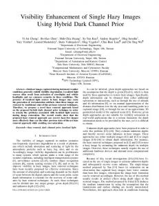
1. Introduction Outdoor images captured in bad weather are prone to yield poor visibility, such as fade surface color, reduced contrast, and blurred scene details (see Figure 1(a)). Thus, removing such negative effects and recovering the realistic clear-day image have strong implications in computer vision applications, such as aerial imagery [1], image classification [2, 3], remote sensing [4], and object recognition [5]. Directly employing traditional image processing techniques [6–9] to enhance the global contrast or local contrast of hazy image is probably the most intuitive and simplest way to recall the visibility of buried regions. But the dehazing effect of these techniques is somehow limited, since the degradation mechanism of hazy image is neglected. By means of the atmospheric scattering model (ASM), subsequent research works [10, 11] mainly concentrate on using multiple images or external information to derive the depth map and the other unknown parameters. Although these techniques are able to achieve impressive results, the prerequisites of

implementation may be difficult to fulfill in many practical cases. Recently, single image dehazing has attracted the most research attentions, and some meaningful significant progress has been made by utilizing powerful image priors. However, these methods may fail under some particular situations. For instance, Fattal [12] presented a transmission estimation method based on the assumption that the surface shading is uncorrelated with the scene transmission in a local patch, whereas this method is unreliable for thick haze image because of the insufficient color information. Zhu et al. [13] proposed the color attenuation prior (CAP) for single image dehazing and create a linear model for modeling the scene depth under this prior, which allows us to directly obtain scene depth. But the constant scattering coefficient may lead to unstable recovery quality, especially for inhomogeneous hazy image. Yoon et al. [14] presented a spatially adaptive dehazing method that merges color histograms with consideration of the wavelength-dependent atmospheric turbidity. However, due to the insufficient wavelength

2

Mathematical Problems in Engineering

(a)

(b)

(c)

(d)

Figure 1: Comparison with the traditional image processing techniques. (a) Hazy image. (b) The result of histogram equalization. (c) The result of multiscale retinex. (d) Our result.

information, this method is challenged when processing dense haze image. Benefiting from prevailing deep learning framework, Cai et al. [15] designed a trainable end-to-end system for the transmission estimation, but the dehazing effect is limited, which may be caused by the insufficient samples that are used to train this system. C. O. Ancuti and C. Ancuti [16] first present a fusion-based dehazing strategy; the main advantage of this method is its linear complexity and it can be implemented in real time, yet the dehazing effect is highly dependent on the haze-feature weight maps. He et al. [17] discovered the dark channel prior (DCP) which is a kind of statistics of the haze-free outdoor images. With this prior and ASM, we can directly estimate the thickness of haze and thus recover visually pleasing result. Unfortunately, DCP approach may not well handle the brightness region where the brightness is inherently similar to the atmospheric light. To deal with this problem, a hybrid DCP was proposed by Huang et al. [18], which also has the ability to circumvent halo effects and to avoid underexposure in the restoration output. Meanwhile, Chen and Huang [19] further developed a dual DCP that uses the big size dark channel and the small size dark channel in order to address the interference of localized light sources. Afterward, Chen et al. [20] provided the Bi-Histogram modification strategy to accurately adjust haze thickness in the transmission map (obtained using DCP) by combining the gamma correction and histogram equalization. In addition to above improved methods, some other techniques [21, 22] were developed to boost the performance. Nevertheless, due to the inaccurate clustering methods, there seems to be no significant improvement on the accuracy of the estimated transmission map. Kim et al. [23] improved the visual clarity by maximizing the contrast information and minimizing information loss in the local patch. Furthermore, Meng et al. [24] proposed an image dehazing method by combining boundary constraint and contextual regularization. The method could exclude image noise and recover the interesting image details and structures. Despite the very

great success for single image dehazing, as we discussed above, almost all the dehazing methods still have two common limitations. That is because the ASM is modeled under the assumption that the illumination is even distributed and the light is scattered only once during the propagation, and we will make more detailed explanation in Section 2. In this paper, based on our previous work [25] and the multiple-scattering theory [26], we redefine a more robust ASM which is more in line with the real world. Further, based on this redefined ASM, a fast single image dehazing algorithm using dual prior knowledge is also proposed. In addition to the positive performance of the redefined ASM, the corresponding dehazing algorithm also has several advantages over the existing state-of-the-art techniques. First, due to the designed scene-wise APSF kernel prediction mechanism, our technique can well eliminate the multiple-scattering effect within each segmented scene. Second, by jointly utilizing the DCP and the maximizing contrast prior (MCP) [27], the ill-posed dehazing problem can be converted into a one-dimensional searching problem, which can effectively decrease the uncertainty of the dehazing problem. Experimental results, as shown in Figure 1, demonstrate that the proposed algorithm achieves better restoration of the edge contrast and color vividness compared with traditional image processing techniques including histogram equalization and the multiscale retinex [8].

2. The Redefined Atmospheric Scattering Model In computer version and computational photography, the ASM proposed by Nayar and Narasimhan [10, 11] is widely used to describe the degradation mechanism of hazy images, and it can be expressed as 𝐼 (𝑥, 𝑦) = 𝐿 ∞ ⋅ 𝜌 (𝑥, 𝑦) ⋅ 𝑡 (𝑥, 𝑦) + 𝐿 ∞ ⋅ (1 − 𝑡 (𝑥, 𝑦)) , (1)

Mathematical Problems in Engineering

3

Scene depth

Scene depth Scene reflection light

Atmospheric light Scattering component

Scene reflection light

Atmospheric light Scattering component

(a)

(b)

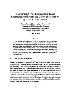
Figure 2: Illustrations of single-scattering effect and multiple-scattering effect. (a) The atmospheric scattering model for single-scattering effect. (b) The atmospheric scattering model for multiple-scattering effect.

where (𝑥, 𝑦) is the pixel index, 𝐼(𝑥, 𝑦) is the input hazy image, 𝐿 ∞ is the atmospheric light which is usually assumed to be a constant [10–24], 𝜌(𝑥, 𝑦) is the scene albedo, and 𝑡(𝑥, 𝑦) is the media transmission. In (1), the first term is named as direct attenuation, which describes how the scene radiance is attenuated by the suspended particles in the medium. The right term is called airlight, which demonstrates the influence of previously scattered light in the imaging procedure. Although the ASM is physically valid under general conditions (see Figure 2(a)), two inner defects of this model still exist: (1) The constant-𝐿 ∞ definition implies that the illuminance is even distributed throughout the entire image, and therefore ASM may not be in accordance with some of the real scenarios. (2) It is well known that the ASM is modeled under the single-scattering assumption; however, the light should be scattered multiple times by the suspended particles before reaching the camera, as can be seen in Figure 2(b). Our previous work [25] has unveiled that the first defect can be addressed by redefining the constant atmospheric light 𝐿 ∞ as the scene-wise variable, which varies spatially but is constant within each scene. To tackle the second limitation, in this paper we introduced the atmospheric point spread function (APSF) [28] to describe influence of multiple scattering and note that both the direct attenuation and airlight must be scattered multiple times during the propagation process. Consequently, a more robust ASM can be redefined as 𝐼 (𝑥, 𝑦) = (𝐿 (𝑖) ⋅ 𝜌 (𝑥, 𝑦) ⋅ 𝑡 (𝑖) + 𝐿 (𝑖) ⋅ (1 − 𝑡 (𝑖))) ∗ ℎ (𝑖)

(𝑥, 𝑦) ∈ Ω𝑖 ,

(2)

where Ω𝑖 is the 𝑖th set of pixel index, ∗ represents the convolution operator, ℎ(𝑖), 𝐿(𝑖), and 𝑡(𝑖) are the scattering kernel, scene illuminance, and scene transmission, respectively, which are all fixed in the 𝑖th index set. Obviously, the proposed ASM is more concise compared with the existing one, while the uneven-illumination problem and the multiple-scattering effect can be well physically explained by introducing scene-wise strategy and APSF.

3. The Proposed Algorithm According to our previous work [25, 29, 30], we can segment a hazy image into 𝑁 nonoverlapping scenes {Ω1 , Ω2 , . . . , Ω𝑁} using 𝑘-means clustering technique and further compute the corresponding haze density {𝑄(1), 𝑄(2), . . . , 𝑄(𝑁)} by assuming that the haze density is constant within each scene (default value of the number of scenes is 𝑁 = 3). Now, the goal of dehazing is to estimate the APSF kernel, scene illuminance, and scene transmission for each scene, which is an ill-posed problem in nature. Fortunately, many image priors have been explored; this inspired us to address this issue by fully leveraging their latent statistical relationship. 3.1. A Scene-Wise APSF Kernel Prediction Mechanism. In [26], Narasimhan and Nayar created an analytic model for the glow around a point source. However, owing to the deconvolution complexity, the convergence of the optimal solution is unreliable for all the optical thickness values. Similar to [28], we introduce the generalized Gaussian distribution model (GGDM) [31] to approximate the APSF, and the modified APSF for neighborhood can be modeled as ℎAPSF (𝑥, 𝑦; 𝑇, 𝑞) =

󵄩𝑘𝑇 󵄨 󵄨𝑘𝑇 󵄩 exp {− 󵄩󵄩󵄩𝑥 − 𝑥, 𝑦 − 𝑦󵄩󵄩󵄩 / 󵄨󵄨󵄨𝐴 (𝑘𝑇, (1 − 𝑞) /𝑞)󵄨󵄨󵄨 } 4 ⋅ Γ2 (1 + 1/𝑘𝑇) ⋅ 𝐴 (𝑘𝑇, (1 − 𝑞) /𝑞)

(3) ,

where (𝑥, 𝑦) is the center index of neighborhood, 𝑞 represents the forward scattering parameter which is correlated with the haze density, 𝑇 = − ln(𝑡) is the optical thickness, 𝑘 is a constant that is correlated with 𝑇 (default value is set as 𝑘 = 0.2), Γ(⋅) is the gamma function, and 𝐴(⋅) represents the scale parameter: 𝐴 (𝑘𝑇,

𝑞2 Γ (1/𝑘𝑇) 1−𝑞 )=√ . 𝑞 Γ (3/𝑘𝑇)

(4)

As aforementioned, the haze density, illuminance, and transmission within each scene are approximately the same,

4

Mathematical Problems in Engineering

and considering the similarity between 𝑞 and 𝑄 within each scene [26], we might as well assume that 𝑞 = 𝑄 for simplicity; thus the scattering kernel for each scene can be simplified as ℎ (𝑖) = 𝑓 (𝑡 (𝑖) , 𝑄 (𝑖)) = ℎAPSF (𝑥, 𝑦; 𝑇 (𝑖) , 𝑞 (𝑖)) ⇐⇒ ℎAPSF (𝑥, 𝑦; − ln (𝑡 (𝑖)) , 𝑄 (𝑖))

(𝑥, 𝑦) ∈ Ω𝑖 ,

(5)

dark 𝜌scene (𝑖) = ( min

where 𝑓 is the simplified APSF description and 𝑇(𝑖) and 𝑞(𝑖) are optical thickness and forward scattering parameter for the 𝑖th scene, respectively. Accordingly, (2) can be rewritten as 𝐼 (𝑥, 𝑦) = (𝐿 (𝑖) ⋅ 𝜌 (𝑥, 𝑦) ⋅ 𝑡 (𝑖) + 𝐿 (𝑖) ⋅ (1 − 𝑡 (𝑖))) ∗ 𝑓 (𝑡 (𝑖) , 𝑄 (𝑖))

(𝑥, 𝑦) ∈ Ω𝑖 .

where 𝑐 is the color channel index and Ω(𝑥, 𝑦) is a local patch centered at (𝑥, 𝑦). Undoubtedly, the information contained in the 𝑖th set of pixel index Ω𝑖 is more sufficient than that contained in Ω(𝑥, 𝑦), so DCP can also be applied to a scenewise strategy and become more robust. Formally, the dark dark (𝑖) can be defined as channel of 𝑖th scene 𝜌scene min 𝜌𝑐 (𝑥󸀠 , 𝑦󸀠 )) 󳨀→ 0.

𝑐∈{𝑅,𝐺,𝐵} (𝑥󸀠 ,𝑦󸀠 )∈Ω𝑖

(8)

Having the scene-based DCP, we can take the min operation in each scene in (6); that is, dark dark 𝐼scene (𝑖) = (𝐿 (𝑖) ⋅ 𝜌scene (𝑖) ⋅ 𝑡 (𝑖) + 𝐿 (𝑖) ⋅ (1 − 𝑡 (𝑖)))

∗ 𝑓 (𝑡 (𝑖) , 𝑄 (𝑖))

(6)

(𝑥, 𝑦) ∈ Ω𝑖 ,

(9)

where 3.2. Model Simplification via DCP. To further alleviate the model complexity, we intend to leverage the relationship between the model parameters using DCP [17]. Let us here recall the dark channel prior (DCP) which is a kind of statistics of the haze-free outdoor images: in most of the nonsky patches, at least one color channel has very low intensity at some pixels (even tends to be zero), and it can be described as

Putting (8) into (9), the scene illuminance 𝐿(𝑖) can be simply estimated as

𝜌𝑐 (𝑥󸀠 , 𝑦󸀠 )) 󳨀→ 0, (7)

For more clarity, we substitute (11) back into (6); thus the function used for restoring the scene albedo can be expressed by

dark 𝜌patch (𝑥, 𝑦) = ( min

min 󸀠

𝑐∈{𝑅,𝐺,𝐵} (𝑥󸀠 ,𝑦 )∈Ω(𝑥,𝑦)

𝜌 (𝑥, 𝑦) =

𝜌 (𝑥, 𝑦)

min 𝐼 (𝑥󸀠 , 𝑦󸀠 )) .

𝑐∈{𝑅,𝐺,𝐵} (𝑥󸀠 ,𝑦󸀠 )∈Ω𝑖

𝐿 (𝑖) =

dark 𝐼scene (𝑖) . (1 − 𝑡 (𝑖)) ∗ 𝑓 (𝑡 (𝑖) , 𝑄 (𝑖))

dark deconv (𝐼 (𝑥, 𝑦) , 𝑓 (𝑡 (𝑖) , 𝑄 (𝑖))) ⋅ (1 − 𝑡 (𝑖)) ∗ 𝑓 (𝑡 (𝑖) , 𝑄 (𝑖)) − 𝐼scene (𝑖) dark 𝐼scene (𝑖) ⋅ 𝑡 (𝑖)

where deconv is the deconvolution operator. Considering the constancy of transmission within each scene, the restoration function is equivalent to

=

dark 𝐼scene (𝑖) = ( min

(𝑥, 𝑦) ∈ Ω𝑖 ,

(13)

(𝑥, 𝑦) ∈ Ω𝑖 .

Since 𝑄(𝑖) can be determined by using our previous work [25], the scene albedo 𝜌 is a function with respect to the scene transmission 𝑡(𝑖), which means that the restoration function can be concisely expressed by 𝜌 (𝑥, 𝑦) = dehaze (𝑡 (𝑖))

(𝑥, 𝑦) ∈ Ω𝑖 .

(14)

3.3. Scene Albedo Restoration Using MCP. On the basis of the maximizing contrast prior (MCP) [27], the contrast for a clear-day image is higher than that of the corresponding

(11)

(12)

hazy one. Therefore, we can estimate the transmission 𝑡(𝑖) by maximizing the contrast within each scene; that is, 𝑡 (𝑖) = argmax {∇𝜌 (𝑥, 𝑦)} = −argmin {∇ (dehaze (𝑡 (𝑖)))}

dark deconv (𝐼 (𝑥, 𝑦) , 𝑓 (𝑡 (𝑖) , 𝑄 (𝑖))) ⋅ (1 − 𝑡 (𝑖)) − 𝐼scene (𝑖) dark 𝐼scene (𝑖) ⋅ 𝑡 (𝑖)

(10)

(𝑥, 𝑦) ∈ Ω𝑖 ,

(15)

where ∇ is gradient operator. To obtain each scene transmission 𝑡(𝑖) accurately, we employ Fibonacci method [32] to solve this one-dimensional searching problem (15). If we remove the haze or fog thoroughly, the recovery results may seem unnatural. Thus, we optionally keep a small amount of haze into the dehazed image by adjusting ̃𝑡(𝑖) = 𝜀 ⋅ 𝑡(𝑖), and we fix 𝜀 = 1.1 in our experiments. Once the transmission map ̃𝑡 has been determined, we can recover the haze-free image via (12). Figures 3(a)–3(c) provide two dehazing examples using the proposed technique. As we can see, due to the 𝐾means clustering technique used in the segmentation process [25], the edge structure of the recovered images is not consistent with that of the input images. This is because image segmentation is inherently a scene-wise process that will blur the edges in the transmission map. Inspired by [25], we utilize

Mathematical Problems in Engineering

(a)

5

(b)

(c)

(d)

(e)

Figure 3: Comparison of dehazing quality before and after refinement via GTV. (a) Hazy images. (b) The transmission maps before edge refinement. (c) The recovered results using (b). (d) The transmission maps after edge refinement. (e) The recovered results using (d).

the guided total variation (GTV) model to increase the edgeconsistency property, and therefore optimal ̃𝑡 can be obtained by solving the following energy function: 󵄩 󵄩2 󵄩 󵄩2 𝐸 (𝑡)̌ = 󵄩󵄩󵄩󵄩𝑡 ̌ − ̃𝑡󵄩󵄩󵄩󵄩2 + 𝜆 1 ⋅ (1 − 𝑊) ⋅ 󵄩󵄩󵄩󵄩∇𝑡󵄩󵄩󵄩󵄩̌ 2 + 𝜆 2 󵄩 󵄩2 ⋅ 𝑊 ⋅ 󵄩󵄩󵄩󵄩∇𝑡 ̌ − ∇𝐼󵄩󵄩󵄩󵄩2 ,

(16)

where guidance image 𝐼 is the gray component of 𝐼, edge weight 𝑊 = 1 − exp(−|∇𝐺|), and 𝜆 1 and 𝜆 2 are regularization parameters (default setting is the same as [25]). As shown in Figures 3(d) and 3(e), the edge-inconsistency problem is well tackled after refinement, the transmission maps are more in line with our intuition, and the corresponding dehazing results are more natural and realistic.

4. Experiments In order to verify the superiority of our dehazing technique, we test it on various types of hazy images and conduct the comparisons with several state-of-the-art dehazing methods, including Tarel and Hautiere [33], He et al. [17], Meng et al. [24], Cai et al. [15], Zhu et al. [13], C. O. Ancuti and C. Ancuti [16], Choi et al. [34], and Wang et al. [35]. All the methods are implemented in MATLAB 2010a on a personal computer with 2.6 GHz Intel(R) Core i5 processor and 8.0 GB RAM. The parameters in our approach are described in Section 3, and the parameters in the eight state-of-the-art dehazing methods are set to be optimal according to [13, 15–17, 24, 33–35] for fair comparison. 4.1. Qualitative Comparison. As all the state-of-the-art dehazing methods are able to generate good results using general hazy images, it is difficult to rank all the dehazing methods visually. Therefore, we carry out these methods on the two benchmark images and five challenging hazy images, including dense haze image, the misty image, the hazy image with large sky region, the hazy image with large scale white/gray region, and the uneven-illumination hazy image. Figure 4 shows the qualitative comparison for different dehazing techniques on these challenging images. The input hazy images are displayed in Figure 4(a); Figures

4(b)–4(j) demonstrate the results of Tarel and Hautiere [33], He et al. [17], Meng et al. [24], Cai et al. [15], Zhu et al. [13], C. O. Ancuti and C. Ancuti [16], Choi et al. [34], Wang et al. [35], and the proposed method, respectively. In Figure 4(b), Tarel and Hautiere’s method utilizes a geometric criterion to tackle the ambiguity between the image color and haze; thus it may fail for the dense haze image (see the third image of Figure 4(b)). As we can see from the fifth image and sixth image of Figure 4(b), halo artifacts can be found nearby the depth jumps, since the involved median filter has poor edge-preserving property. In addition, the color of the sky region in the fifth image in Figure 4(b) is significantly distorted; this is because the estimated atmospheric veil is an extreme case based on the DCP and therefore the transmission will be overestimated inevitably. As shown in Figure 4(c), He et al.’s method can produce reasonable dehazing results for most images. However, DCP cannot be applied to the region where the brightness is similar to the atmospheric light; thus the sky region in the fifth image of Figure 4(c) is obviously overenhanced. Similarly, the results of Meng et al.’s method also suffer from the more serious overenhancement phenomenon. The reason can be explained: the boundary constraint could not address the limitation of DCP and the depth-local-constant assumption that uses 3×3 block is bound to further reduce the robustness of DCP (see the fifth image in Figure 4(d)). As we observed in Figures 4(e) and 4(f), although Cai et al.’s method and Zhu et al.’s method can avoid the overenhancement and halo artifacts by adopting these learning strategies, haze residual can be found in the third and fifth images of Figures 4(e) and 4(f). Furthermore, Cai et al.’s method is not reliable when processing the single-tone image (color shifting is noticeable in the third image of Figure 4(e)). It can be found in Figures 4(g) and 4(h) that C. O. Ancuti and C. Ancuti’s method and Choi et al.’s method may not work well once the hazy image is dark or haze is dense; this is because the accuracy of the weight maps is challenged when severe dark aspects of the preprocessed image dominate, especially in the third image of Figures 4(g) and 4(h). In Figure 4(i), the removing haze ability of Wang et al.’s method is relatively modest, since the control factor is set as a constant empirically. Besides, all the above methods cannot well handle the uneven-illumination

6

Mathematical Problems in Engineering

The first benchmark image

The second benchmark image

Dense haze image

Misty image

Hazy image with large sky region

Hazy image with large scale white/gray region

Uneven-illumination hazy image (a)

(b)

(c)

(d)

(e)

(f)

(g)

(h)

(i)

(j)

Figure 4: Qualitative comparison of different methods on challenging hazy images. (a) Hazy image. (b) Tarel and Hautiere’s results. (c) He et al.’s results. (d) Meng et al.’s results. (e) Cai et al.’s results. (f) Zhu et al.’s results. (g) C. O. Ancuti and C. Ancuti’s results. (h) Choi et al.’s results. (i) Wang et al.’s results. (j) Ours.

hazy image (the shadow regions in the seventh row of Figure 4 still look dim after restoration). In contrast, our technique successfully unveils the more scene details of the shadow regions. More importantly, our technique yields better visibility for all the experimental hazy images by eliminating the multiple-scattering effect, as shown in Figure 4(j). 4.2. Quantitative Comparison. In order to perform quantitative evaluation and rate these algorithms, we adopt several widely used indicators, including the percentage of new visible edges 𝐸, contrast restoration quality 𝑅, Fog Aware Density Evaluator (FADE), Structural Similarity (SSIM), mean squares error (MSE), and color fidelity (𝐻). According to [36], indicator 𝐸 measures the ratio of newly visible edges after restoration, and 𝑅 is a metric that verifies the mean ratio of the gradients at visible edges. The indicator FADE is proposed by [34], which is an assessment of haze removal ability. SSIM [37] is used for evaluating the ability to maintain the edge structural information of the dehazing methods.

MSE indicates the average difference between the recovered result and the real haze-free image (or ground truth image). 𝐻 [38] is used to measure the degree of color retention for the restored image. In general, higher values of 𝐸, 𝑅, and SSIM or the lower values of FADE, MSE, and 𝐻 imply better visual improvement after restoration. Figure 5 shows the recovery results of different methods on the four synthetic hazy images which are synthesized based on the Stereo Datasets [39–41] and ASM. In Figure 5, from left to right, we show synthesized hazy images, the results of Tarel and Hautiere [33], He et al. [17], Meng et al. [24], Cai et al. [15], Zhu et al. [13], C. O. Ancuti and C. Ancuti [16], Choi et al. [34], Wang et al. [35], and the proposed method, as well as the ground truth images for fair comparison. The corresponding quantitative assessment results for the dehazing results shown in Figure 5 are depicted in Figure 6. Analyzing the data of Figures 6(a) and 6(b), our dehazing results achieve the top values of FADE and 𝑅 for all the hazy images, which means that the images recovered using

Mathematical Problems in Engineering

7

Table 1: Time consumption comparison between Tarel and Hautiere, He et al., Meng et al., Cai et al., Zhu et al., C. O. Ancuti and C. Ancuti, Choi et al., Wang et al., and our method. Image resolutionTarel and Hautiere 100 × 100 0.5580 200 × 200 0.7541 300 × 300 1.5729 400 × 400 3.2726 500 × 500 6.4017 600 × 600 15.9577 700 × 700 18.5932 800 × 800 30.3173 900 × 900 47.8541 1000 × 1000 67.6774

He et al. Meng et al. 0.7715 1.1450 0.8435 1.2730 0.9335 1.4819 0.9727 1.7164 1.0755 1.9791 1.2508 2.3356 1.4849 2.7702 1.6843 2.9401 1.8191 3.3742 2.0667 3.8347

Cai et al. Zhu et al. C. O. Ancuti and C. Ancuti Choi et al. Wang et al. 0.6981 0.2041 1.4599 2.6727 0.6912 0.9136 0.2776 1.6819 5.8877 0.7597 1.4969 0.3271 1.8652 10.4068 0.7982 2.6782 0.4538 2.2550 17.0303 0.8512 3.9295 0.5292 2.8496 26.8812 0.8745 5.5260 0.7959 3.1234 37.3098 0.9258 7.2436 1.0236 3.3229 52.7681 0.9541 9.3592 1.4342 4.0019 74.4012 0.9916 12.8897 1.5354 4.7334 91.5810 1.0297 14.3210 1.9078 5.4656 118.3491 1.0689

Ours 0.2415 0.4078 0.6174 0.8223 1.0418 1.2588 1.3945 1.5082 1.7412 1.8872

(a)

(b)

(c)

(d)

Figure 5: Quantitative comparison of different methods on synthetic and real-world hazy images. From left to right: hazy images, Tarel and Hautiere’s results, He et al.’s results, Meng et al.’s results, Cai et al.’s results, Zhu et al.’s results, C. O. Ancuti and C. Ancuti’s results, Choi et al.’s results, Wang et al.’s results, and our results and the ground truth images.

the proposed approach contain more information of target details. According to Figure 6(c), our results yield the top value for Figures 5(b) and 5(c), and our method achieves the second top or third top value for Figures 5(a) and 5(d), but the results must be balanced because the number of recovered visible edges can be increased by noise amplification. For instance, Tarel and Hautiere’s results have the highest value for Figure 5(a), whereas the overenhancement can be noticed in the cup and head of sculpture. As can be seen in Figure 6(d), the average MSE values of the recovery results of the proposed technique are relatively larger than others. This is because our method has the illumination compensation ability that may cause the difference between the recovery result and the ground truth image. For the rest of indicators, as shown in Figures 6(e) and 6(f), our method outperforms other methods in general, which proves the outstanding dehazing effect of the proposed technique. The computational complexity is another important evaluation factor for a dehazing method. In Table 1, we provide the time consumption comparison between Tarel and

Hautiere [33], He et al. [17] (accelerated using the guided image filtering [42]), Meng et al. [24], Cai et al. [15], Zhu et al. [13], C. O. Ancuti and C. Ancuti [16], Choi et al. [34], Wang et al. [35], and our method for the images with different resolution. As we can see, the proposed technique is much faster than those of Tarel and Hautiere [33], Cai et al. [15], C. O. Ancuti and C. Ancuti [16], and He et al. [17, 42]. Although our method is slightly slower than Zhu et al. [13] and Wang et al. [35], the dehazing quality of our method is obviously better than that of Zhu et al. [13] and Wang et al. [35]. In summary, the proposed technique has a better application prospect compared to the other methods, and we attribute these advantages to the improved ASM and the corresponding dehazing strategy.

5. Discussion and Conclusions In this paper, by taking the uneven-illumination condition and the multiple-scattering effect into consideration, we have proposed a more robust ASM to overcome the inherent

8

Mathematical Problems in Engineering 6

0.9 0.8

5

0.7

2

4

0.6

1.5

0.5

R 3

0.4

E 1

Figure 5(d)

Figure 5(a)

Tarel and Hautiere

Cai et al.

Choi et al.

Tarel and Hautiere

Cai et al.

Choi et al.

Tarel and Hautiere

Cai et al.

Choi et al.

He et al.

Zhu et al.

Wang et al.

He et al.

Zhu et al.

Wang et al.

He et al.

Zhu et al.

Wang et al.

Meng et al.

C. O. Ancuti and C. Ancuti

Ours

Meng et al.

C. O. Ancuti and C. Ancuti

Ours

Meng et al.

C. O. Ancuti and C. Ancuti

Ours

(a)

(b)

(c)

1

0.14

0.25

0.9

0.12

0.8

0.1

0.7

0.08

0.6

SSIM

0.06

0.2 0.15 H

0.5 0.4

0.1

0.3

0.04

0.2

0.02

0.05

0.1 0

Figure 5(d)

Figure 5(c)

Figure 5(b)

Figure 5(a)

Figure 5(d)

0 Figure 5(c)

Figure 5(d)

Figure 5(c)

Figure 5(b)

Figure 5(a)

0

Figure 5(a)

MSE

Figure 5(c)

0 Figure 5(d)

0 Figure 5(a)

0.5

Figure 5(d)

Figure 5(c)

Figure 5(b)

Figure 5(a)

0

1

Figure 5(c)

0.1

Figure 5(b)

0.2

Figure 5(b)

2

0.3

Figure 5(b)

FADE

2.5

Tarel and Hautiere

Cai et al.

Choi et al.

Tarel and Hautiere

Cai et al.

Choi et al.

Tarel and Hautiere

Cai et al.

Choi et al.

He et al.

Zhu et al.

Wang et al.

He et al.

Zhu et al.

Wang et al.

He et al.

Zhu et al.

Wang et al.

Meng et al.

C. O. Ancuti and C. Ancuti

Ours

Meng et al.

C. O. Ancuti and C. Ancuti

Ours

Meng et al.

C. O. Ancuti and C. Ancuti

Ours

(d)

(e)

(f)

Figure 6: Quantitative comparison of recovered images shown in Figure 5. (a) Fog Aware Density Evaluator of different algorithms. (b) Contrast restoration quality of different algorithms. (c) The percentage of new visible edges of different algorithms. (d) The mean squares error of different algorithms. (e) The structural similarity of different algorithms. (f) The color fidelity of different algorithms.

limitation of the existing one. Based on this redefined ASM, a fast single image dehazing method has been further presented. In this method, we can effectively eliminate the multiple-scattering effect within each segmented scene via the proposed scene-wise APSF kernel prediction mechanism. Moreover, by sufficiently utilizing the existing prior knowledge, the dehazing problem can be subtly converted into a one-dimensional searching problem, which allows us to directly estimate the scene transmission and thereby recover a visually realistic result via the proposed ASM. The extensive experimental results have revealed the advance of the proposed technique compared with several state-of-theart alternatives.

Conflicts of Interest The authors declare that there are no conflicts of interest regarding the publication of this paper.

Acknowledgments This study was supported in part by the National Natural Science Foundation of China [61571241], IndustryUniversity-Research Prospective Joint Project of Jiangsu Province [BY2014014], Key University Science Research Project of Jiangsu Province [15KJA510002], and Postgraduate

Mathematical Problems in Engineering Research & Practice Innovation Program of Jiangsu Province [KYLX16_0665].

References [1] G. Woodell, Z. Rahman, S. E. Reichenbach et al., “Advanced image processing of aerial imagery,” in Proceedings of the Defense and Security Symposium, Orlando, Fla, USA, 2006, 62460E–62460E. [2] L. Shao, L. Liu, and X. Li, “Feature learning for image classification via multiobjective genetic programming,” IEEE Transactions on Neural Networks and Learning Systems, vol. 25, no. 7, pp. 1359–1371, 2014. [3] S. L. Zhang and T. C. Chang, “A Study of Image Classification of Remote Sensing Based on Back-Propagation Neural Network with Extended Delta Bar Delta,” Mathematical Problems in Engineering, vol. 2015, Article ID 178598, 2015. [4] J. Han, D. Zhang, G. Cheng, L. Guo, and J. Ren, “Object detection in optical remote sensing images based on weakly supervised learning and high-level feature learning,” IEEE Transactions on Geoscience and Remote Sensing, vol. 53, no. 6, pp. 3325– 3337, 2015. [5] Z. Zhang and D. Tao, “Slow feature analysis for human action recognition,” IEEE Transactions on Pattern Analysis and Machine Intelligence, vol. 34, no. 3, pp. 436–450, 2012. [6] T. K. Kim, J. K. Paik, and B. S. Kang, “Contrast enhancement system using spatially adaptive histogram equalization with temporal filtering,” IEEE Transactions on Consumer Electronics, vol. 44, no. 1, pp. 82–87, 1998. [7] J. A. Stark, “Adaptive image contrast enhancement using generalizations of histogram equalization,” IEEE Transactions on Image Processing, vol. 9, no. 5, pp. 889–896, 2000. [8] Z.-U. Rahman, D. J. Jobson, and G. A. Woodell, “Multi-scale retinex for color image enhancement,” in Proceedings of the 1996 IEEE International Conference on Image Processing, ICIP’96. Part 2 (of 3), pp. 1003–1006, September 1996. [9] S. Lee, “An efficient content-based image enhancement in the compressed domain using retinex theory,” IEEE Transactions on Circuits and Systems for Video Technology, vol. 17, no. 2, pp. 199– 213, 2007. [10] S. K. Nayar and S. G. Narasimhan, “Vision in bad weather,” in Proceedings of the 7th IEEE International Conference on Computer Vision (ICCV ’99), vol. 2, pp. 820–827, IEEE, Kerkyra, Greece, September 1999. [11] S. G. Narasimhan and S. K. Nayar, “Contrast restoration of weather degraded images,” IEEE Transactions on Pattern Analysis and Machine Intelligence, vol. 25, no. 6, pp. 713–724, 2003. [12] R. Fattal, “Single image dehazing,” ACM Transactions on Graphics, vol. 27, no. 3, article 72, 2008. [13] Q. Zhu, J. Mai, and L. Shao, “A fast single image haze removal algorithm using color attenuation prior,” IEEE Transactions on Image Processing, vol. 24, no. 11, pp. 3522–3533, 2015. [14] I. Yoon, S. Jeong, J. Jeong, D. Seo, and J. Paik, “Wavelengthadaptive dehazing using histogram merging-based classification for UAV images,” Sensors, vol. 15, no. 3, pp. 6633–6651, 2015. [15] B. Cai, X. Xu, K. Jia, C. Qing, and D. Tao, “DehazeNet: An end-to-end system for single image haze removal,” IEEE Transactions on Image Processing, vol. 25, no. 11, pp. 5187–5198, 2016. [16] C. O. Ancuti and C. Ancuti, “Single image dehazing by multiscale fusion,” IEEE Transactions on Image Processing, vol. 22, no. 8, pp. 3271–3282, 2013.

9 [17] K. He, J. Sun, and X. Tang, “Single image haze removal using dark channel prior,” IEEE Transactions on Pattern Analysis and Machine Intelligence, vol. 33, no. 12, pp. 2341–2353, 2011. [18] S.-C. Huang, B.-H. Chen, and Y.-J. Cheng, “An efficient visibility enhancement algorithm for road scenes captured by intelligent transportation systems,” IEEE Transactions on Intelligent Transportation Systems, vol. 15, no. 5, pp. 2321–2332, 2014. [19] B.-H. Chen and S.-C. Huang, “An advanced visibility restoration algorithm for single hazy images,” ACM Transactions on Multimedia Computing, Communications, and Applications (TOMM), vol. 11, no. 4, 2015. [20] B.-H. Chen, S.-C. Huang, and J. H. Ye, “Hazy image restoration by bi-histogram modification,” ACM Transactions on Intelligent Systems and Technology, vol. 6, no. 4, article 50, 2015. [21] Y. Li, Q. Miao, J. Song, Y. Quan, and W. Li, “Single image haze removal based on haze physical characteristics and adaptive sky region detection,” Neurocomputing, vol. 182, pp. 221–234, 2016. [22] B. Jiang, W. Zhang, J. Zhao et al., “Gray-scale image Dehazing guided by scene depth information,” Mathematical Problems in Engineering, vol. 2016, Article ID 7809214, 10 pages, 2016. [23] J.-H. Kim, W.-D. Jang, J.-Y. Sim, and C.-S. Kim, “Optimized contrast enhancement for real-time image and video dehazing,” Journal of Visual Communication and Image Representation, vol. 24, no. 3, pp. 410–425, 2013. [24] G. Meng, Y. Wang, J. Duan, S. Xiang, and C. Pan, “Efficient image dehazing with boundary constraint and contextual regularization,” in Proceedings of the 14th IEEE International Conference on Computer Vision (ICCV ’13), pp. 617–624, IEEE, Sydney, Australia, December 2013. [25] M. Ju, D. Zhang, and X. Wang, “Single image dehazing via an improved atmospheric scattering model,” The Visual Computer, 2016. [26] S. Narasimhan and S. Nayar, “Shedding light on the weather,” in Proceedings of the CVPR 2003: Computer Vision and Pattern Recognition Conference, pp. I-665–I-672, Madison, WI, USA. [27] R. T. Tan, “Visibility in bad weather from a single image,” in Proceedings of the 26th IEEE Conference on Computer Vision and Pattern Recognition (CVPR ’08), pp. 1–8, Anchorage, Alaska, USA, June 2008. [28] R. He, Z. Wang, Y. Fan, and D. Dagan Feng, “Multiple scattering model based single image dehazing,” in Proceedings of the 2013 IEEE 8th Conference on Industrial Electronics and Applications, ICIEA 2013, pp. 733–737, aus, June 2013. [29] Z. Gu, M. Ju, and D. Zhang, “A Single Image Dehazing Method Using Average Saturation Prior,” Mathematical Problems in Engineering, vol. 2017, Article ID 6851301, 2017. [30] M. Ju, Z. Gu, and D. Zhang, “Single image haze removal based on the improved atmospheric scattering model,” Neurocomputing, vol. 260, pp. 180–191, 2017. [31] S. Metari and F. Deschˆenes, “A new convolution kernel for atmospheric point spread function applied to computer vision,” in Proceedings of the 2007 IEEE 11th International Conference on Computer Vision, ICCV, bra, October 2007. [32] K. J. Overholt, “Efficiency of the Fibonacci search method,” BIT Journal, vol. 13, no. 1, pp. 92–96, 1973. [33] J. Tarel and N. Hautiere, “Fast visibility restoration from a single color or gray level image,” in Proceedings of the IEEE 12th International Conference on Computer Vision (ICCV ’09), pp. 2201–2208, September 2009. [34] L. K. Choi, J. You, and A. C. Bovik, “Referenceless prediction of perceptual fog density and perceptual image defogging,” IEEE

10

[35]

[36]

[37]

[38]

[39]

[40]

[41]

[42]

Mathematical Problems in Engineering Transactions on Image Processing, vol. 24, no. 11, pp. 3888–3901, 2015. W. Wang, X. Yuan, X. Wu, and Y. Liu, “Fast Image Dehazing Method Based on Linear Transformation,” IEEE Transactions on Multimedia, vol. 19, no. 6, pp. 1142–1155, 2017. ´ Dumont, “Blind N. Hauti`ere, J.-P. Tarel, D. Aubert, and E. contrast enhancement assessment by gradient ratioing at visible edges,” Image Analysis and Stereology, vol. 27, no. 2, pp. 87–95, 2008. Z. Wang, A. C. Bovik, H. R. Sheikh, and E. P. Simoncelli, “Image quality assessment: from error visibility to structural similarity,” IEEE Transactions on Image Processing, vol. 13, no. 4, pp. 600– 612, 2004. D. J. Jobson, Z. ur Rahman, and G. A. Woodell, “Statistics of visual representation,” in Proceedings of the Visual Information Processing XI, vol. 4736 of Proceedings of SPIE, pp. 25–35, Orlando, Fla, USA, 2002. D. Scharstein and R. Szeliski, “High-accuracy stereo depth maps using structured light,” in Proceedings of the IEEE Computer Society Conference on Computer Vision and Pattern Recognition (CVPR ’03), vol. 1, pp. I-195–I-202, IEEE, June 2003. D. Scharstein and C. Pal, “Learning conditional random fields for stereo,” in Proceedings of the IEEE Computer Society Conference on Computer Vision and Pattern Recognition (CVPR ’07), IEEE, Minneapolis, Minn, USA, June 2007. D. Scharstein and R. Szeliski, “A taxonomy and evaluation of dense two-frame stereo correspondence algorithms,” International Journal of Computer Vision, vol. 47, no. 1–3, pp. 7–42, 2002. K. He, J. Sun, and X. Tang, “Guided image filtering,” IEEE Transactions on Pattern Analysis and Machine Intelligence, vol. 35, no. 6, pp. 1397–1409, 2013.

Advances in

Operations Research Hindawi Publishing Corporation http://www.hindawi.com

Volume 2014

Advances in

Decision Sciences Hindawi Publishing Corporation http://www.hindawi.com

Volume 2014

Journal of

Applied Mathematics

Algebra

Hindawi Publishing Corporation http://www.hindawi.com

Hindawi Publishing Corporation http://www.hindawi.com

Volume 2014

Journal of

Probability and Statistics Volume 2014

The Scientific World Journal Hindawi Publishing Corporation http://www.hindawi.com

Hindawi Publishing Corporation http://www.hindawi.com

Volume 2014

International Journal of

Differential Equations Hindawi Publishing Corporation http://www.hindawi.com

Volume 2014

Volume 2014

Submit your manuscripts at https://www.hindawi.com International Journal of

Advances in

Combinatorics Hindawi Publishing Corporation http://www.hindawi.com

Mathematical Physics Hindawi Publishing Corporation http://www.hindawi.com

Volume 2014

Journal of

Complex Analysis Hindawi Publishing Corporation http://www.hindawi.com

Volume 2014

International Journal of Mathematics and Mathematical Sciences

Mathematical Problems in Engineering

Journal of

Mathematics Hindawi Publishing Corporation http://www.hindawi.com

Volume 2014

Hindawi Publishing Corporation http://www.hindawi.com

Volume 2014

Volume 2014

Hindawi Publishing Corporation http://www.hindawi.com

Volume 2014

#HRBQDSDĮ,@SGDL@SHBR

Journal of

Volume 201

Hindawi Publishing Corporation http://www.hindawi.com

Discrete Dynamics in Nature and Society

Journal of

Function Spaces Hindawi Publishing Corporation http://www.hindawi.com

Abstract and Applied Analysis

Volume 2014

Hindawi Publishing Corporation http://www.hindawi.com

Volume 2014

Hindawi Publishing Corporation http://www.hindawi.com

Volume 2014

International Journal of

Journal of

Stochastic Analysis

Optimization

Hindawi Publishing Corporation http://www.hindawi.com

Hindawi Publishing Corporation http://www.hindawi.com

Volume 2014

Volume 2014