Vision-based Kinematic Modelling of Some Parallel Manipulators for

Proceedings of EuCoMeS, the first European Conference on Mechanism Science Obergurgl (Austria), February 21–26 2006 Manfred Husty and Hans-Peter Schr¨ocker, editors

Vision-based Kinematic Modelling of Some Parallel Manipulators for Control Purposes Nicolas Andreff∗

Philippe Martinet∗

In this paper, it is recalled that computer vision, used as an exteroceptive redundant metrology mean, simplifies the control of a Gough-Stewart parallel robot. Indeed, contrary to the usual methodology where the robot is modeled independently from the control law which will be implemented, we take, since the early modeling stage, into account that vision will be used for control. Hence, kinematic modeling and projective geometry are fused into a control-devoted vision-based kinematic model through the observation of its legs. Thus, this novel vision-based kinematic modeling is extended to two other parallel manipulator families, namely Orthoglide and I4L. Inspired by the geometry of lines, this kind of model unifies and simplifies both identification and control. Indeed, it has a reduced parameter set and yields a linear solution to calibration. Using the same models, visual servoing schemes are presented, where the directions of the non-rigidly linked legs are servoed, rather than the end-effector pose.

1 Introduction Parallel mechanisms are such that there exist several kinematic chains (or legs) between their base and their mobile platform (or end-effector). Therefore, they may exhibit a better repeatability (see Merlet (2000)) than serial mechanisms but not a better accuracy, as stated in Wang and Masory (1993), because of the large number of links and passive joints. There can be two ways to compensate for the low accuracy. The first way is to perform a kinematic calibration of the mechanism and the second one is to use a control law which is robust to calibration errors. The latter is the ultimate goal of the present work. There exists a large amount of work on the control of parallel mechanisms 1 . Let us immediately discard joint control, since it does not take into account the kinematic closures and may therefore FR TIMS - CNRS 2856, UBP-CNRS-IFMA, 27 avenue des Landais, 63177 Aubi`ere Cedex, France [email protected] 1 See http://www-sop.inria.fr/coprin/equipe/merlet for a long list of references.

∗

1

EuCoMeS 1st European Conference on Mechanism Science

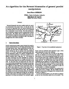
(a) Gough-Stewart platform

(b) Orthoglide

(c) I4L

Figure 1: The manipulators studied in this paper, here equipped with a visual target for calibration purposes. yield high internal forces (see Dasgupta and Mruthyunjaya (1998)). Moreover, since there may exist several end-effector poses associated to a given joint configuration, a simple joint control may converge to the wrong end-effector pose, even though it converges to the correct joint configuration. Alternately, Cartesian control consists in computing at each sample time the instantaneous Cartesian velocities that drive an adequate error signal to zero. Actuation is then naturally achieved through the use of the differential inverse kinematic model which transforms Cartesian velocities into admissible joint velocities. Usually, the error signal is made of the current and desired end-effector pose, which appears in the inverse differential kinematic model of parallel mechanisms (while for serial mechanisms the latter only depends on the joint values). Consequently, one needs be able to estimate or measure the end-effector pose. As far as we know, all the effort has been put on the estimation of the end-effector pose through the forward kinematic model and the joint measurements. However, this yields much trouble, related to the fact that there is usually no closed-form expression of the forward kinematic model of a parallel mechanism. Hence, one numerically inverts the inverse kinematic model, which has a closed-form expression for most of the parallel mechanisms. However, it is known (see Merlet (1990) or Husty (1996)) that this numerical inversion requires high order polynomial root determination, with several possible solutions: Dietmaier (1998) identified up to 40 real solutions for a Gough-Stewart platform (introduced by Gough and Whitehall (1962) and Stewart (1965)). Much of the work is thus devoted to solving this problem accurately and in real-time (see for instance Zhao and Peng (2000)) or to designing parallel mechanisms with algebraic forward kinematic model, such as the ones by Kim and Tsai (2002) or Gogu (2004). Alternately, one of the promising paths lies in the use of the so-called metrological redundancy introduced by Baron and Angeles (1998), which simplifies the kinematic models by introducing additional sensors into the mechanism and thus yields easier control as in Marquet (2002). Computer vision being an efficient way of estimating the end-effector pose, it is a good alternative to use it for Cartesian control of parallel mechanisms. It can be done in two correct manners. Visual servoing First, one can perform visual servoing (see Espiau et al. (1992)) by using the measured end-effector pose directly in the error signal as in Martinet et al. (1996), thus relieving oneself from the forward kinematic problem. This is the choice made by Koreichi et al.

2

N. Andreff and P. Martinet.: Vision-based Kinematic Modelling . . . for Control Purposes

(1998), Kino et al. (1999) and Kallio et al. (2000) (for parallel robots with a reduced number of degrees of freedom), by observation of the robot end-effector and the use of standard kinematic models. A novel approach However, the previous approach consists solely in a simple adaptation of now classical control schemes, which, although very efficient, are not very innovative. Moreover, the direct application of visual servoing techniques assumes implicitly that the robot inverse differential kinematic model is given and that it is calibrated. Therefore, modeling, identification and control have small interaction with each other. Indeed, the model is usually defined for control using proprioceptive sensing only and does not foresee the use of vision for control, then identification and control are defined later on with the constraints imposed by the model. This is useful for modularity but this might not be efficient in terms of accuracy as well as of experimental set-up time. On the opposite, a unified framework for modeling, identification and control, apart from being definitely more satisfying for the mind, would certainly open a path to higher efficiency. Indeed, instead of having identification and control being driven by the initial modeling stage, one could have a model taking into account the use of vision for control and hence for identification. To do so, it is necessary to fuse robot kinematics and projective geometry into a projective kinematic model. Thus, we propose a novel third way to use vision, which gathers the advantages of redundant metrology and visual servoing while avoiding most of their drawbacks. Moreover, observing the end-effector of a parallel mechanism by vision may be incompatible with its application. For instance, it is not wise to imagine observing the end-effector of a machining tool. On the opposite, it should not be a problem to observe the legs of the mechanism, even in such extreme cases. Thereby, vision would be turned from an exteroceptive sensor to a somewhat more proprioceptive sensor. This brings us back to the redundant metrology paradigm. Parallel mechanisms are most often designed with slim and rectilinear legs. Therefore, the line geometry (described in Pl¨ ucker (1865); Semple and Kneebone (1952)) is certainly the heart of the unification, all the more as line geometry is also widely used in computer vision as in Faugeras (1993) and has already been used for visual servoing as in Andreff et al. (2002); Mahony and Hamel (2005). Previous work on kinematic calibration by Renaud et al. (2005) already considered vision as a way to deliver contact-less metrological redundancy. However, to the exception of Renaud et al. (2004), the models that were calibrated remain classical. Indeed, vision was only used for sensing and neither modeling nor control was questioned from the vision point of view. A first step in this direction was made in Andreff et al. (2005) were vision was used already at the modeling stage in order to derive a visual servoing scheme based on the observation of the leg directions of a Gough-Stewart parallel robot. Consequently, the contribution of this paper is to present an additional step towards an original and unifying vision-based modeling and identification and control framework of parallel mechanisms by observing their legs with a camera fixed with respect to the base. Vision-based modeling of a Gough-Stewart platform is recalled then extended to two other classes of parallel mechanisms: the Orthoglide from Wenger and Chablat (2002) and the I4L from Krut et al. (2003) (Figure 1).

3

EuCoMeS 1st European Conference on Mechanism Science

2 Preliminaries The present work assumes that the vision system is calibrated, which is not anymore a strong hypothesis, since accurate and easy-to-use camera calibration software can easily be found on the Web2 . Since we plan to use line geometry as a central element for modeling, a representation for lines suited to control and identification is needed. Among the work on visual servoing from lines found in Espiau et al. (1992); Andreff et al. (2002); Mahony and Hamel (2005); Malis et al. (2002), we prefer the so-called Bi-normalized Pl¨ ucker coordinates representation in Andreff et al. (2002) which turns out to be coherent with kinematic modeling of parallel mechanisms. In such a representation, a straight line in the 3D space, being oriented according to Stolfi (1991), is modeled by the triplet (u, h, h) where u is the unit vector giving the spatial direction of the line, h is also a unit vector and h is a non-negative scalar. They are defined by hh = −−→ OP × u where O is the center of projection and P is any point on the line. Notice that, using this notation, the well-known (normalized) Pl¨ ucker coordinates used in Pl¨ ucker (1865); Pottmann et al. (1998) are the couple (u, hh) . An interesting property of this representation is that h = (hx , hy , hz )T represents the image projection of the line, i.e. the equation of the image line verifies hx x + h y y + h z = 0

(1)

where x and y are the coordinates of a point in the image. The interpretation of the scalar h is the orthogonal distance of the line to the center of projection.

3 Vision-based kinematics of a Gough-Stewart platform Consider the hexapod in Figure 1(a). It has 6 legs of varying length qi , i ∈ 1..6, attached to the base by spherical joints located in points Ai and to the moving platform (end-effector) by spherical joints located in points Bi . The inverse kinematic model of such an hexapod is given by −−−→ −−−→ ∀i ∈ 1..6, qi2 = Ai Bi T Ai Bi (2) −−−→ expressing that qi is the length of vector Ai Bi . This model can be expressed in any Euclidean reference frame. Hence, it can be expressed in the base frame Rb , in the end-effector frame Re or in the camera frame Rc . Hereafter, the reference frame in which vectors and points are expressed will be denoted by a left upper-script. Notice that, slightly abusively, c Ai denotes both the coordinates in Rc of −−−→ point Ai and those of vector Oc Ai , where Oc is the origin of Rc . The Euclidean transformation from frame i to frame j will be denoted by its rotation matrix i Rj and its translation vector i t . According to Andreff et al. (2005) and assuming a calibrated camera, one can express the j vision-based kinematics of the hexapod in the camera frame. To do so, instead of the inverse kinematic model, we used the so-called implicit kinematic model, suggested by Wampler et al. (1995), which relates the end-effector pose and the joint values in an invariant form expressing 2

See for instance http://www.vision.caltech.edu/bouguetj/calib doc/.

4

N. Andreff and P. Martinet.: Vision-based Kinematic Modelling . . . for Control Purposes

the kinematic closure constraints. However, rather than using a scalar invariant form as it is usually done, we use a vector invariant form: q i c ui = c R e e B i + c t e − c A i

(3)

where c ui , i = 1..6 are the unit vectors giving the direction of each leg in the camera frame. Differentiating it with respect to time and knowing that c ui , i = 1..6 are unit vectors (i.e. cu ˙ Ti c ui = 0) yields the vision-based differential inverse kinematic model

c q˙ = c Dinv τc c

with

= MTi c τc

with

cu ˙

i

 uT1 (c A1 × c u1 )T   .. c inv Dc = −  ...  . c uT ( c A × c u ) T 6 6 6 ¡ ¤ ¢ £ 1 MTi = − I3 − c ui c uTi I3 −[c Ai + qi c ui ]× qi c

(4)

(5)

where c τc is the Cartesian velocity of the camera frame, considered as attached to the base frame and moving with respect to a fixed end-effector, expressed in itself and []× denotes the antisymmetric matrix associated to the vector cross-product. Then, assuming cylindrical legs and extracting their edges (c hei 1 and c hei 2 ) from the image, one can reconstruct the direction of each leg by c

ui =

c h e1 i kc hei 1

× c hei 2 × c hei 2 k

(6)

and use it together with (4) and (5) to derive a control law of the form: +

d T diag(q)E q˙ = −λc\ Dinv c N

(7)

with E = (eT1 , ..., eT6 )T , ei = c ui × c udi , NT = (N1 , ..., N6 )T , NTi = [c udi ]× MTi , and where the hat means that only an estimate can be used. For instance, this estimate can be chosen as the the matrix expressed at convergence or computed at each iteration from sensor information. Discussion From (3), it is clearly easier to recover the end-effector pose knowing the direction of the legs than their lengths, since more equations are available. Moreover, the solution to this problem can be found using linear algebra as proved by Baron and Angeles (1998). Hence, it is wiser to sense direction than the length. It can be done in two ways: the first one is by using extra joint sensors together with either an accurate calibration step or a careful mechanical design, the second one is to use vision which can directly measure the direction in space. However, if one gets rid of length sensing, the length appearing in (5) is not any more available at control time, but Andreff and Martinet (2005) showed that a constant average length can be used instead without loss of accuracy. In conclusion, observing the leg directions of the Gough-Stewart platform is enough to uniquely define its end-effector pose and to perform Cartesian control. The purpose of the next two sections is to establish, for two other parallel mechanisms, the equivalence between the endeffector pose and adequate vision observation, as well as the differential models associated to the latter, paving the way for their future control.

5

EuCoMeS 1st European Conference on Mechanism Science

4 Vision-based kinematics of the Orthoglide family The Orthoglide, shown in Figure 1(b) and introduced by Wenger and Chablat (2002), is a parallel manipulator with 3 perpendicular linear joints. Each joint is linked to the end-effector by an articulated parallelogram. From this mechanism, a whole family can be derived by relaxing the orthogonality assumption. To establish the inverse kinematic model of parallel mechanisms, one often expresses kinematic chain closure around a given element of the mechanism. For instance, in the Gough-Stewart case, it is done around the length-varying legs. In the case of the Orthoglide family, although Wenger and Chablat (2002) obtain the kinematic model more easily when the joint axes are orthogonal, one may apply the same methodology and close the kinematic chain around the articulated parallelogram of each leg. As seen above in the Gough-Stewart case, it is preferable to express the kinematic closure in vector form (rather than in scalar form, so that one keeps the ability to choose the optimal sensing method). One can express this constraint: −−−→ A i B i = L i ui (8) in any reference frame, where Ai is the attachment point of the parallelogram onto the ith linear joint, Bi the attachment point onto the end-effector, L is the equivalent length of the parallelogram and ui is the unit vector from Ai to Bi . Using Ai = Oi + qi zi where zi is the direction of the ith joint axis and Oi is its origin (defined by the zero of the sensor), as well as the fact that Bi has a constant expression in the end-effector frame, one can express (8) in any reference frame R∗ as: ∗

Re e Bi + ∗ te − ∗ Oi − qi ∗ zi = Li ∗ ui

(9)

where it shall be noticed that ∗ Re is constant by design. Consequently, the terms ∗ Re e Bi and ∗ O merge into a single kinematic parameter ∗ C = ∗ O − ∗ R e B . i i i e i Since the parallelograms are made of two cylinders with square section, it is here again very easy to measure ui directly in the camera frame and the above expression can be instantiated in the camera frame, to obtain the vision-based implicit kinematic model of the Orthoglide: c

te − c Ci − qi c zi = Li c ui

(10)

where {c Ci , c zi , Li , i = 1..3} form the kinematic parameter set to be calibrated, here in the camera frame rather than in the base frame. Note that calibration becomes a linear problem if one measures c te , qi and c ui . Once again, one shall notice that it is easier to solve for the forward kinematic problem if one measures the leg directions but not the joint displacements (intersection of 3 lines) than if one measures the joint displacements but not the leg directions (intersection of 3 spheres). Nevertheless, the main point in (10) is that knowing the leg directions is equivalent to knowing the end-effector pose. Time differentiating (10) yields: c

ve − q˙i c zi = Li c u˙ i

(11)

Since ui is a unit vector, it is orthogonal to its time derivative, thus: c Tc ve ui

− q˙i c zTi c ui = 0

6

(12)

N. Andreff and P. Martinet.: Vision-based Kinematic Modelling . . . for Control Purposes

The above two expressions yield the vision-based differential inverse kinematic model: q˙i = c

u˙ i =

c uT i c ve c zT c u i i µ ¶ c z c uT 1 i i c ve I3 − c T c Li zi ui

(13) (14)

which is singular when the parallelogram of any leg is embedded in the orthogonal plane to the same leg joint axis. Discussion Recall that Cartesian control can be achieved in three ways. In the first standard case, the control feedback consists of the end-effector pose obtained by solving the forward kinematic problem, thus requiring the calibration of the full kinematic parameter set. In the second case known as 3D pose visual servoing Martinet et al. (1996), the control feedback consists of the end-effector pose measured by vision, thus requiring to fix a visual target onto the end-effector as well as camera calibration and end-effector to visual target calibration (also known as hand-eye calibration) but reducing the set of kinematic parameters to be calibrated to { c zi , i = 1..3} since the only required kinematic knowledge lies in (13) to convert the end-effector velocity obtained by the visual servoing control law into joint velocities. Finally, in the third case, the control feedback consists of the leg direction measurements, thus yielding:   ˆ + c u1 − c uref M1 1 ref  c ˆ 2  (15) ve = −λ M c u2 − c u2  , λ > 0 c u − c uref ˆ3 M 3 3 ˆ i , i = 1..4 are estimates of the matrices in equation (14). Actual joint actuation is then where M obtained using (13). In such a scheme, one needs to calibrate the camera and the kinematic parameters { c zi , Li , i = 1..3} since both (13) and (14) are used for control, but one is relieved from adding a visual target and from hand-eye calibration. Moreover, as the leg lengths Li act as gains in the control, they can be replaced here also by their CAD value without any loss of accuracy. Consequently, this third scheme is the one requiring minimal instrumentation and calibration burden.

5 Vision-based kinematics of the I4L family The I4L robot, shown in (Figure 1(c)) and introduced in Krut et al. (2003), is a parallel manipulator composed of 4 parallel linear joints, aligned by pairs (Figure 2(a)). Each joint is linked to the end-effector by an articulated parallelogram. Moreover, the moving nacelle is separated into two parts (Figure 2(b)), whose relative translation T is transformed into a proportional end-effector rotation θ = T /K. From this mechanism, a whole family can be derived by relaxing the parallelism and alignment assumptions. Here again, we express the closure of the kinematic chains around each parallelogram yielding the same equation as (9), with the same notation transposed to the I4L. Here, we take into account the articulated nacelle by: Bi = E + (δi Kθ + ²i S)xb + σi Dyb

7

(16)

EuCoMeS 1st European Conference on Mechanism Science q4

q3

B3 A3

A4 2S

B3 B1

A1

y b x b O q1

B4 2D B2 L

B4 y

xe

e

y

ze E(X, θ Y, Z)

2H

A2

B1

B

zb xb B2

T

q2

(a) Global kinematic description

(c) Motions leaving the leg directions constant.

(b) Articulated nacelle

Figure 2: I4L mechanism geometry with E, the end-effector position, δ3 = δ4 = ²2 = ²4 = σ3 = σ4 = 1, δ1 = δ2 = 0, ²1 = ²3 = σ1 = σ2 = −1 and the other notation defined in Figure 2. Then, the implicit kinematic model in vector form is Li ui = E + δi Kθxb + ²i S xb + σi Dyb − Oi −qi zi (17) {z } | Ci =CST

for which exists a unique solution to (E, θ, qi , i = 1..4) when ui , i = 1..4 are measured and adequate calibration of (K, S, D, Li , Ci , zi , i = 1..4), which is here again a linear problem, is done. However, the above result is not true in the configuration presented in Krut et al. (2003) where all joint axes are parallel, which yields a two dimensional solution subspace (shown in Figure 2(c)) to (17). Leaving that point for a short while, one comes back to almost the same point as for the Orthoglide and one can derive the vision-based differential inverse kinematic model of the I4L, expressed in the camera frame: µ ¶ c uT ¡ ¢ c ve i c I 3 δ i K xb q˙i = c T c (18) ω zi ui ¶ µ ¶ µ c z c uT ¡ ¢ c ve 1 i i c c I3 δi K xb (19) I3 − c T c u˙ i = ω Li zi ui where ω is the angular velocity of the end-effector frame around the constant zb axis. Using the latter expression, one can use a control law similar to (15) provided that the set uref i , i = 1..4 is equivalent to the end-effector pose, i.e. that (17) admits a unique solution: µc

ve ω

¶

    ˆ 1 + c u − c uref M 1 1     .. = −λ  ...   ,λ > 0 . ref c c ˆ M4 u − u 4

(20)

4

ˆ i , i = 1..4 are estimates of the matrices in equation (19). where M In the configuration introduced in Krut et al. (2003) where the actuator axes are all parallel (i.e. zi = ±xb , ∀i), equation (18) becomes ³ ´ µc v ¶ c uT c y c uT c z e i b i b q˙i = 1 ± c uT c x ± c uT c x δi K (21) ω b b i i This is the expression of the differential inverse kinematic model of the I4L which was reported in Renaud et al. (2004), where the signs depend on the assembly direction of each actuator. In

8

N. Andreff and P. Martinet.: Vision-based Kinematic Modelling . . . for Control Purposes

the same configuration, equation (19) becomes c

u˙ i =

1 ³ I3 − Li

c x c uT b i c xT c u i b

0

´ µc v ¶ e

(22)

ω

which is coherent with the fact that only translations of the nacelle along y b and zb modify the leg directions, while a translation of the nacelle along xb do not (see Figure 2(c)) and a rotation of the end-effector corresponds to a relative translation of the two halves of the nacelle, obtained by globally translating the planar sub-mechanism (A1 A2 B2 B1 ), see Figure 2(a). The control proposed in (20) was simulated in two configurations: when all the joints are parallel and when joints 2 and 4 are lifted upwards in order to make a 5 degree angle with respectively joints 1 and 3 (Figure 3(a)). The initial end-effector pose is defined by b E = (0.5, 0.1, −1)T , T = −0.1 and the desired one by b E = (0, 0, −0.5)T , T = 0. Figure 5 displays the time evolution of the error between the current end-effector pose and the desired one in the two cases. In the non singular case, even though only the leg directions are controlled, the endeffector pose converges to the desired one. However, in the parallel case, only the components along b y and b z converge, while the position along b x and the rotation around b z are not affected by the control, as expected. 0.6

X

0.4

Y

Z

0.2 (meters)

0.20

−0.50

−1.20 −1.1

Z

0

T

−0.2 −0.4

0.0

−0.6

Y −1.9 1.1

0

20

0.0 X

40

60

80

(iteration number)

100

120

1.9

(a) Non singular configuration

(b) Time evolution of the pose error while controlling the leg directions of an I4L like robot: parallel (dashed) and non singular (solid) configurations

Discussion Here again, the kinematic model was expressed in a vector invariant form −−−−−−−−−→ Ai (q)Bi (b Te ) = Li ui

(23)

from which we exhibited a differential kinematic model relating the end-effector Cartesian velocity to the time derivative of the leg directions and to the joint velocities, using a reduced set of kinematic parameters. This control can be achieved without measuring the actuated joint values, but rather the leg directions in space, which can easily be done by vision. However, in the case where all joints are parallel, the equivalence between leg directions and end-effector pose is lost. Does that mean that the vision-based modeling fails in the case where all joint axes are parallel ? No, but we need to go a bit deeper into projective geometry and consider the second component hi of the Bi-normalised Pl¨ ucker coordinates of the lines Li

9

EuCoMeS 1st European Conference on Mechanism Science

passing through Ai and Bi . Indeed, to separate the various solutions in Figure 2(c) even though the joint axes were hidden, the reader would use the image of the mechanism legs and more specifically the image of Li , i = 1..4, which is exactly hi as stated in section 2. Similarly, a camera placed above the mechanism will record the projection of each leg onto the image, from which it is rather easy, under the cylindrical leg assumption, to extract both ui and hi . Then, another step is required for control, which requires deriving a closed form expression for the time derivative of the latter unit vectors, but not for the vectors themselves since such an expression is complex and useless. However, this is the matter of a future paper.

6 Conclusions In this paper, we have confirmed that it is not wise to measure the actuated joint values to perform easy kinematic analysis and control of parallel mechanisms. Instead, it is wiser to measure adequately chosen internal values, namely the direction of the legs. This corresponds more or less to measuring passive joint values. However, since these directions are essentially spatial quantities, it would require tedious mechanical design to measure them using standard joint sensors, and we prefer to use vision, which is a tool perfectly suited to that task. Doing so, we have also confirmed that implicit kinematic models in vector form should be preferred to scalar inverse kinematic models. Measuring by vision the leg directions, we thus can measure the differential kinematic model rather than estimate it through solving for the forward kinematic problem. This reduces drastically the computational cost as well as the size of the kinematic parameter set, although these parameters are not intrinsically related to the mechanism but depend also on the relative location of the camera with respect to the mechanism. However, taking this global approach, we could express a vision-based kinematic model which is suited to the control of parallel mechanisms, without needing any static kinematic model. Moreover, this work shows not only that, as in the other fields of robotics, vision is efficient, but even better that vision and parallel mechanisms form a natural couple.

Acknowledgement This study was jointly funded by CPER Auvergne 2003-2005 program, by the CNRS-ROBEA program through the MP2 project and the EU-IP project NEXT no. NMP2-CT-2005-011815 .

References N. Andreff, B. Espiau, and R. Horaud. Visual servoing from lines. Int. Journal of Robotics Research, 21(8):679–700, Aug. 2002. N. Andreff, A. Marchadier, and P. Martinet. Vision-based control of a Gough-Stewart parallel mechanism using legs observation. In Proc. Int. Conf. Robotics and Automation (ICRA’05), pages 2546–2551, Barcelona, Spain, May 2005. N. Andreff and P. Martinet. Visual servoing of a Gough-Stewart parallel robot without proprioceptive sensors. In Fifth Int. Workshop on Robot Motion and Control (RoMoCo’05), Dymaczewo, Poland, June 23-25 2005.

10

N. Andreff and P. Martinet.: Vision-based Kinematic Modelling . . . for Control Purposes

L. Baron and J. Angeles. The on-line direct kinematics of parallel manipulators under jointsensor redundancy. In Advances in Robot Kinematics, pages 126–137. Kluwer, 1998. B. Dasgupta and T. Mruthyunjaya. Force redundancy in parallel manipulators: theoretical and practical issues. Mech. Mach. Theory, 33(6):727–742, 1998. P. Dietmaier. The Stewart-Gough platform of general geometry can have 40 real postures. In J. Lenarˇciˇc and M. L. Husty, editors, Advances in Robot Kinematics: Analysis and Control, pages 1–10. Kluwer, 1998. B. Espiau, F. Chaumette, and P. Rives. A New Approach To Visual Servoing in Robotics. IEEE Trans. on Robotics and Automation, 8(3), June 1992. O. Faugeras. Three-Dimensional Computer Vision - A Geometric Viewpoint. Artificial intelligence. MIT Press, Cambridge, MA, 1993. G. Gogu. Fully-isotropic T3R1-type parallel manipulator. In J. Lenarˇciˇc and C. Galletti, editors, On Advances in Robot Kinematics, volume Kluwer Academic Publishers, pages 265–272. 2004. V. Gough and S. Whitehall. Universal tyre test machine. In Proc. FISITA 9th Int. Technical Congress, pages 117–137, May 1962. M. Husty. An algorithm for solving the direct kinematics of general Gough-Stewart platforms. Mech. Mach. Theory, 31(4):365–380, 1996. P. Kallio, Q. Zhou, and H. N. Koivo. Three-dimensional position control of a parallel micromanipulator using visual servoing. In B. J. Nelson and E. Jean-Marc Breguet, editors, Microrobotics and Microassembly II, Proceedings of SPIE, volume 4194, pages 103–111, Boston, USA, Nov. 2000. H. Kim and L.-W. Tsai. Evaluation of a Cartesian parallel manipulator. In J. Lenarˇciˇc and F. Thomas, editors, Advances in Robot Kinematics: Theory and Applications. Kluwer Academic Publishers, June 2002. H. Kino, C. Cheah, S. Yabe, S. Kawamua, and S. Arimoto. A motion control scheme in task oriented coordinates and its robustness for parallel wire driven systems. In Int. Conf. Advanced Robotics (ICAR’99), pages 545–550, Tokyo, Japan, Oct. 25-27 1999. M. Koreichi, S. Babaci, F. Chaumette, G. Fried, and J. Pontnau. Visual servo control of a parallel manipulator for assembly tasks. In 6th Int. Symposium on Intelligent Robotic Systems, SIRS’98, pages 109–116, Edimburg, Scotland, July 1998. S. Krut, O. Company, M. Benoit, H. Ota, and F. Pierrot. I4: A new parallel mechanism for scara motions. In Proceedings of the 2003 International Conference on Robotics and Automation, Taipei, Taiwan, 2003. R. Mahony and T. Hamel. Image-based visual servo control of aerial robotic systems using linear image features. IEEE Transactions on Robotics, 21(2):227–239, Apr. 2005.

11

EuCoMeS 1st European Conference on Mechanism Science

E. Malis, J. Borrelly, and P. Rives. Intrinsics-free visual servoing with respect to straight lines. In IEEE/RSJ Int. Conf. on Intelligent Robots Systems, pages 384–389, Lausanne, Switzerland, Oct. 2002. F. Marquet. Contribution a ` l’´etude de l’apport de la redondance en robotique parall`ele. PhD thesis, LIRMM - Univ. Montpellier II, Oct. 2002. P. Martinet, J. Gallice, and D. Khadraoui. Vision based control law using 3d visual features. In Proc. World Automation Congress, WAC’96, Robotics and Manufacturing Systems, volume 3, pages 497–502, Montpellier, France, May 1996. J.-P. Merlet. An algorithm for the forward kinematics of general 6 d.o.f. parallel manipulators. Technical Report 1331, INRIA, Nov. 1990. J.-P. Merlet. Parallel robots. Kluwer Academic Publishers, 2000. J. Pl¨ ucker. On a new geometry of space. Philosophical Transactions of the Royal Society of London, 155:725–791, 1865. H. Pottmann, M. Peternell, and B. Ravani. Approximation in line space – applications in robot kinematics and surface reconstruction. In J. Lenarˇciˇc and M. L. Husty, editors, Advances in Robot Kinematics: Analysis and Control, pages 403–412. Kluwer Academic Publishers, 1998. P. Renaud, N. Andreff, P. Martinet, and G. Gogu. Kinematic calibration of parallel mechanisms: A novel approach using legs observation. IEEE Transactions on Robotics, 2005. In press. P. Renaud, N. Andreff, F. Pierrot, and P. Martinet. Combining end-effector and legs observation for kinematic calibration of parallel mechanisms. In IEEE Int. Conf. on Robotics and Automation (ICRA 2004), pages 4116–4121, New Orleans, USA, May 2004. J. Semple and G. Kneebone. Algebraic Projective Geometry. Oxford Science Publication, 1952. D. Stewart. A platform with six degrees of freedom. In Proc. IMechE (London), volume 180, pages 371–386, 1965. J. Stolfi. Oriented Projective Geometry. Academic Press, 1991. C. Wampler, J. Hollerbach, and T. Arai. An implicit loop method for kinematic calibration and its application to closed-chain mechanisms. IEEE Transactions on Robotics and Automation, 11(5):710–724, 1995. J. Wang and O. Masory. On the accuracy of a Stewart platform - Part I: The effect of manufacturing tolerances. In IEEE Int. Conf. on Robotics and Automation (ICRA 1993), pages 114–120, 1993. P. Wenger and D. Chablat. Design of a three-axis isotropic parallel manipulator for machining applications: The orthoglide. In C. Gosselin and I. Ebert-Uphoff, editors, Proc. of the Workshop on Fundamental Issues and Future Research Directions for Parallel Mechnanisms and Manipulators, Quebec City, October 2002. X. Zhao and S. Peng. Direct displacement analysis of parallel manipulators. Journal of Robotics Systems, 17(6):341–345, 2000.

12