human and monkey visual subordinate categorization strat- egies. Neither the humans nor ... embedded in a very high-dimensional space hampers the detailed ...
Visual Categorization and Object Representation in Monkeys and Humans N. Sigala1 , F. Gabbiani2 , and N. K. Logothetis1
Abstract & We investigated the influence of a categorization task on the extraction and representation of perceptual features in humans and monkeys. The use of parameterized stimuli (schematic faces and fish) with fixed diagnostic features in combination with a similarity-rating task allowed us to demonstrate perceptual sensitization to the diagnostic dimensions of the categorization task for the monkeys. Moreover, our results reveal important similarities between
INTRODUCTION A basic cognitive capacity of primates, as well as of many other species, is the ability to make sense of the perceptual world by discriminating features and categorizing objects. The goal of our experiments was to gain insight into the mechanisms underlying this capacity. Monkeys, whose visual system is similar to that of humans (Van Essen, Drury, Joshi, & Miller, 1998) are ideal subjects for such research, because they are adept at a variety of visual discrimination tasks and are capable of some stimulus generalization (Fabre-Thorpe, Richard, & Thorpe, 1998; Neiworth & Wright, 1994). They are, therefore, excellent models for combined behavioral and electrophysiological approaches. A few studies have systematically tried to elucidate the ways that features are extracted and represented by nonhuman primates in the context of a categorization task (Delorme, Richard, & Fabre-Thorpe, 2000; Vogels, 1999a, 1999b; Sugihara, Edelman, & Tanaka, 1998; Sands, Lincoln, & Wright, 1982). These studies have shown that rhesus monkeys are capable of representing natural objects at basic (e.g., trees vs. nontrees; Vogels, 1999a, 1999b) or superordinate (animals or food; Delorme et al., 2000; Fabre-Thorpe et al., 1998; Sands et al., 1982) levels, and that they can recover a low-dimensional configuration of a set of artificial objects built into a high-dimensional parameter space, based on their objective similarity (Sugihara et al., 1998). However, the use of either uncontrolled stimulus sets or of stimuli
1
Max-Planck Institute for Biological Cybernetics, College of Medicine © 2002 Massachusetts Institute of Technology
2
Baylor
human and monkey visual subordinate categorization strategies. Neither the humans nor the monkeys compared the new stimuli to class prototypes or based their decisions on conditional probabilities along stimulus dimensions. Instead, they classified each object according to its similarity to familiar members of the alternative categories, or with respect to its position to a linear boundary between the learned categories. &
embedded in a very high-dimensional space hampers the detailed investigation of fine discriminations. Consequently, it still remains to be shown which features of the objects are represented and how these representations are affected by categorization. For a more detailed study of visual object categorization and representation, we employed a subordinate classification task. Subordinate categories are defined by small changes in the perceptible details of the stimuli, making them harder to distinguish than basic categories. As such, a subordinate categorization task is suitable for the study of feature extraction and representation. By adopting a well-studied stimulus set (Brunswik faces; Brunswik & Rieter, 1938) as well as a novel one (fish outlines), we were able to compare our results from humans and rhesus monkeys with those of influential human psychophysical studies on categorization (Nosofsky, 1991; Reed, 1972).
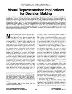
RESULTS Stimuli, Tasks, and Models of Categorization The stimuli were line drawings of faces or fish. Each schematic face consisted of an outline and four varying dimensions: the eye height (EH), the eye separation (ES), the nose length (NL), and the mouth height (MH). Each dimension could take three discrete values (34 = 81 possible combinations). The schematic fish also had four variable dimensions, namely the shape of the dorsal fin (DF), tail (T), ventral fins (VF), and mouth (M). Figure 1a and b depicts the three different values that each dimension could take for face and fish outlines, respectively. The patterns on the left consist of the Journal of Cognitive Neuroscience 14:2, pp. 187- 198
a
2
1
3
b
c 2 1 Eye height
3 Mouth height
Eye separation
3 2 1 Nose length
Figure 1. Parameterized variation of stimulus features. (a) The first stimulus set consisted of Brunswik faces differing along four dimensions: eye height (EH), eye separation (ES), nose length (NL), and mouth height (MH). Each dimension took three discrete values. Three examples are illustrated from left to right with minimal, intermediate and maximal values for all four dimensions, respectively. (b) The second stimulus set consisted of fish outlines and also varied along four dimensions, namely the shape of the dorsal fin (DF), tail (T), ventral fins (VF), and mouth (M). In this case also, each dimension took three discrete values. From left to right: minimal, intermediate and maximal value for all four dimensions, respectively. (c) Graphical representation of the four dimensions characterizing the face stimuli. Eye and mouth heights were measured from face center. Stimuli in (a) labeled accordingly in (c). Grid intersection points represent all possible stimuli (9 £ 9 = 81) obtained from combinations of three discrete values along each dimension.
minimum feature values, the ones in the middle of the intermediate values and the ones on the right of the maximum values. (The size difference from minimum to medium and from medium to maximum values for any dimension of the face outlines corresponds to 0.38 in visual angle). The 4-D vectors of parameters characterizing each stimulus were represented by their projections onto two 2-D plots consisting of the first two dimensions (EH, ES for faces; DF, T for fish) and the last two dimensions (NL, MH for faces; VF, M for fish). Figure 1c shows the projections of the left (1), middle (2), and right (3) faces of Figure 1a. The first task of the subjects was to rate 20 stimuli from each set for their similarity following a protocol of triad comparisons (see Methods). Three stimuli were presented simultaneously (as in Figure 1a and b) and the subjects had to compare the pattern in the middle with the one on its right and on its left. They indicated which one was more similar to it by pressing a corresponding lever. The subjects’ responses were first converted to a 188
Journal of Cognitive Neuroscience
matrix of pairwise dissimilarities between the stimuli. These dissimilarities were then used to find a 4-D configuration of 20 vectors whose pairwise Euclidean distances best approximated them (see Methods). This psychophysical representation of the stimuli could then be directly compared with the original, physical one. Figure 2a illustrates the original, physical configuration of 20 faces along 2 £ 2 projections. The labeling and colors are related to the design of the following separate task that the subjects had to perform. For this second task, the subjects initially learned to classify 10 stimuli (training exemplars) in two categories (see Methods for training protocol). In the next phase, the subjects categorized another 10, and later 24, novel stimuli (test exemplars). The physical configuration of the training and of 10 (out of 24) test exemplars can be seen in Figure 2a. The red circles correspond to the training exemplars of one class and the yellow circles to the training exemplars of the other class. The first two test exemplars were the prototype of each category (purple circles; labeled 1 and 2), formed by averaging the dimension values of the five corresponding training exemplars. The blue circles illustrate eight further test exemplars chosen to span a large area of the stimulus space between and around the training exemplars. The categories were chosen to be separable along two of the four dimensions of the stimuli. Specifically, for Brunswik faces, they were separable along the (EH, ES), but not along the (NL, MH), dimensions (Figure 2a, solid line). For fish outlines, they were separable along (DF, T), but not along (VF, M). Linear separability is a prerequisite for the prototype and boundary models to operate, although there is no evidence that natural categories conform to linear separability (Medin & Schaffer, 1978), or that linearly separable categories are learned more readily than nonlinearly separable ones (Medin & Schwanenflugel, 1981). However, it has been argued that linear classification may be a very natural decision strategy, albeit not constraining for the human classification ability (Ashby & Gott, 1988). To evaluate the strategy used by subjects during classification of stimulus patterns, a total of seven models were fitted to the experimental classification probabilities. They can be broadly divided into prototype, exemplar, boundary, and probability-based models (see Methods for mathematical descriptions). Prototype models postulate that subjects classify stimuli by comparing their similarity to the prototypes of each category (Figure 2b). Two different prototype models were tested. The weighted prototype similarity model (WPSM; Nosofsky, 1991) assumes that similarity decays exponentially with distance and that distance is weighted along each stimulus dimension according to the attention that it receives from the subject. The weighted prototype model (WPM; Reed & Friedman 1973; Reed, 1972), on Volume 14, Number 2
0.9 Eye separation
b
1.0 2
1
Boundary model
3
1
0.8 0.7 3 4 5 0.6 0.5
25
34
1 2
28
7
1345
0.2 0.3 0.4 0.5 0.6 0.7 0.6 Mouth height
Prototype model
16
Eye height 16 34
1
3138
0.8
0.3
Exemplar model
Cue Validity model
2
0.7
0.9
Dimension 2
a
1
4
24 7
1973) takes in addition into account the relative frequency of appearance of each stimulus dimension value during the training session. The questions that can be addressed by assessing these models are: (1) How do the categorization data of the two species compare? (2) Are there differences in goodness of fit for the data between the broad classes of models? (3) Is the exponential decrease of similarity with distance necessary to explain the categorization performance? (4) Do the scaled distances derived from the subjects’ responses improve the fit of the models?
2 2 25
5
0.4 0.5 0.6 Nose length
54 0.7 Dimension 1
Figure 2. Distribution of stimuli and models of categorization. (a) Plot of dimension values taken by 20 schematic faces used both for similarity and categorization tasks (see Figure 1c). Training exemplars (labeled 1- 5) for Category 1 and 2 are represented by red and yellow circles, respectively. Note that the 2-D representation of two different stimuli may overlap. The first two test exemplars (purple circles) were prototypes for Categories 1 and 2 (labeled accordingly). Blue circles: eight test exemplars used during the transfer phase of the categorization task. Note that the two categories were linearly separable along the (EH, ES) dimensions (solid line) but not along the (NL, MH) dimensions (see Figure 1 for abbreviations). (b) Models of subject categorization performance in terms of physical or psychophysical stimulus dimension values. Prototype models (1) postulate that test exemplars are categorized according to their similarity to class prototypes whereas exemplar models (2) assume that similarity to each training exemplar is taken into account. Boundary models (3) assume that a decision boundary underlies categorization performance whereas cue validity models (4) rely on diagnostic feature values along each dimension.
the other hand, assumes a linear decay of similarity with weighted distance. Exemplar models postulate that subjects classify stimuli by computing their similarity to all category exemplars (Figure 2c). We tested the generalized context model (GCM; Nosofsky, 1991) that assumes exponential decay of similarity with weighted distance and the average distance model (ADM; Reed, 1972; Reed & Friedman, 1973), where similarity decays linearly with weighted distance. In boundary models, the stimuli are categorized according to their position with respect to a boundary in stimulus space (Figure 2d). The model tested was the probit linear model (PBI; Ashby & Gott, 1988; Finney, 1971), which posits a hyperplane as boundary. Finally, probability models assume that the subject uses the conditional probability of category ownership based on the stimulus values along each dimension (Figure 2e). In the weighted cue validity model (WCVM; Reed, 1972; Reed & Friedman, 1973), these conditional probabilities are weighted by the attention assigned to each dimension, while the weighted frequency cue validity model (WFCVM; Reed, 1972; Reed & Friedman,
Psychophysical Stimulus Representation Before and After Categorization To investigate how the subjects’ representation of the stimuli was affected by categorization, we collected similarity ratings before and after the categorization task was performed. Figure 3a illustrates the resulting psychophysical representation of face stimuli (triangles) for one monkey prior to the categorization task. Patterns perceived as more similar are closer on the corresponding 2-D plots, while the ones that are perceived as less similar are further apart. The relationship between psychophysical (triangles) and physical (circles) stimuli is indicated by the length of the line segments connecting corresponding points. Clearly, this monkey did not represent any of the dimensions in a consistent way, resulting in a configuration that did not capture the physical distinctiveness of the stimuli, despite its well-above chance performance at the matching control task (71%, chance: 50%, for a 2AFC task). In contrast, the human subject illustrated in Figure 3c was able to extract and represent the different dimensions distinctly and veridically with respect to the original configuration. A second set of similarity ratings was collected after the subjects learned to categorize the stimuli. The resulting psychophysical representations are illustrated in Figure 3b and d for the same subjects as in Figure 3a and c, respectively. The human subject’s representation did not change and was again closely related to the physical stimulus configuration along all four dimensions. In contrast, the monkey’s representation became closer to the physical configuration, particularly along Dimensions 1 and 2, which were the diagnostic dimensions for the preceding categorization task. To quantify this effect, the distances between psychophysical and physical stimuli along Dimensions 1 and 2 (¢ 12) and Dimensions 3 and 4 (¢ 34) were averaged over all stimuli before and after categorization. They are reported in Figure 4a (mean ± SEM) for the same monkey and human subjects of Figure 3. As may be seen from the figure, the psychophysical representation of the human subject before categorization was more faithful to the physical stimuli (corresponding to lower distance differences) than the monkey’s representation ( p < .005, Sigala, Gabbiani, and Logothetis
189
a
0.9
0.7
0.8 0.7
0.7
0.8 0.7
0.8
0.8
0.5 0.2 0.3 0.4 0.5 0.6 0.7
b
Monkey, after cat.
0.9
0.9 0.3
0.4
0.5
0.6
0.7
0.6 0.7
0.8 0.7
Eye separation
0.6 Mouth height
0.6 Eye separation
Human, before categorization 0.6
0.9
0.5 0.2 0.3 0.4 0.5 0.6 0.7
d
Human, after cat.
0.9
0.7
0.6
0.3
0.4
0.5
0.6
0.7
0.4
0.5
0.6
0.7
0.6 0.7
0.8
0.8
Mouth height
0.9
c
Monkey, before categorization 0.6
0.8
0.6 0.9
0.5 0.2 0.3 0.4 0.5 0.6 0.7
0.9
0.5 0.3
0.4
Eye height
0.5
0.6
0.7
Nose length
0.2 0.3 0.4 0.5 0.6 0.7 Eye height
0.3
Nose length
Figure 3. Psychophysical representation of face stimuli. Stimulus representation for a single monkey subject before (a) and after (b) categorization (triangles: psychophysical representation based on similarity ratings; circles: physical stimulus values). Lines connect matching psychophysical and physical stimulus representations. When several patterns share the same combination of physical dimension values, multiple triangles are connected to the same circle. Longer lines correspond to less faithful psychophysical representation of corresponding physical stimulus values. Color code as in Figure 2. Normalized fit stress sn = 0.0095 and 0.0145, respectively. Psychophysical and physical representations before (c) and after (d) categorization for a single human subject. Normalized fit stress: sn = 0.0077 and 0.0059, respectively.
paired t test; Smith- Satterthwaite statistics). No statistically significant change in the human representation
Distance difference
a
0.1
**
0
b
1 0.5 0
190
before cat. after cat.
0.2 faces
12 34 Monkey
12 34 Human
occurred following categorization ( p > .41), while the monkey’s representation of the first two dimensions significantly improved ( p < .005; Figure 4a, **) and was indistinguishable from the human one ( p > .15). A similar decrease in ¢ 12 but not in ¢ 34 after categorization was observed in a second monkey. Similarly, ¢ 12 and ¢ 34 remained unchanged in data pooled from three human subjects before categorization when compared to five subjects pooled after categorization, confirming the single subject result. In the case of the fish stimuli, data pooled from two monkeys tested before and after categorization showed the same improvement in the representation of the two diagnostic dimensions ( p < .005; Figure 4b, **) while the representation of Dimensions 3 and 4 was unaffected ( p > .19; Figure 4b). In contrast, the human
fish *
** 12 34 Monkey
12 34 Human
Journal of Cognitive Neuroscience
Figure 4. Effects of categorization on the representation of the stimuli. (a) Mean distance difference between psychophysical and physical stimuli along the (EH, ES) dimensions (¢ 12) and the (NL, MH) dimensions (¢ 34) before and after categorization averaged over 20 schematic faces (error bars are standard error of mean). Same monkey and human subjects as in Figure 3. (b) Average distance difference along the (DF, T) and (VF, M) dimensions before and after categorization for fish outlines. Data before and after categorization taken from two different monkeys and a single human subject. See Figure 1 for abbreviations. Significance levels (t test): ** corresponds to p < .005 and * to p < .01.
Volume 14, Number 2
a
Monkeys 1
Observed Probability
subject depicted in Figure 4b showed an increase in the distance difference, ¢ 34, along Dimensions 3 and 4 ( p < .01; Figure 4b, *) corresponding to a less faithful representation of the ventral fin and mouth of the fish. A similar result was observed in data pooled from four human subjects tested before categorization of fish stimuli when compared to five different subjects tested afterwards. Thus, the humans showed a selective decrease in perceptual sensitivity to the nondiagnostic dimensions of the fish stimuli. To minimize the possibility that the stimulus configurations based on the subjects’ similarity ratings were obtained by chance, we compared them to random configurations generated in Monte Carlo simulations (see Methods). For Brunswik faces, the monkey and human configurations were on average 11 and 15 times closer to the physical than to random configurations, respectively. This supports the conclusion that they reflect the subjects’ internal representation of the stimuli.
1
GCM
WPSM
0.8
0.8
0.6
0.6
0.4
0.4
0.2 0
0
1
-ln(L)= 69.9 0.2 0.4 0.6 0.8 1
0.2 0 1
PBI
0.8
0.6
0.6
0.4
0.4
0
b
0
Humans 1
-ln(L)= 73.0 0.2 0.4 0.6 0.8 1
0.2 0
0.6
0.6
The categorization strategies adopted by monkeys and humans were investigated by fitting the parameters of categorization models to experimental probabilities using maximum likelihood. Overall, the models performed similarly for monkeys and humans for both stimulus size sets (20 or 34). In Figure 5 each plot reports the observed categorization probabilities versus the ones predicted by the model. Thus, a perfect fit would correspond to all points falling along the diagonal (dashed lines in Figure 5) and, conversely, the worst fits are those with the largest scatter of points around the diagonal. For both monkeys and humans, the exemplar models best fit the data, followed by the boundary, prototype and probability models. Similar results were obtained with 20 faces, as illustrated by the log-likelihoods reported in Table 1. The higher performance of the generalized context model was corroborated in humans by pairwise comparisons of model log-likelihoods pooled across different subjects and face stimuli: The GCM performed significantly better than the probability model (WFCVM; p < .002, Wilcoxon signed rank test for paired observations, 19 experiments). It also performed significantly better than the prototype model on the same data set ( p < .002). To further rule out the WPSM, we considered more closely the classification probabilities of the two prototypes and of two test faces (7 and 8, Figure 2a) that had similar distances to the exemplars but eccentric spatial positions (Nosofsky, 1991; Reed, 1972). A bad fit of the GCM probabilities for these faces would support a prototype categorization strategy. The GCM, however, predicted these classification probabilities as accurately as the WPSM. Thus, it appears unlikely that humans or
0.4
0.4
Observed Probability
Categorization of Face and Fish Stimuli by Monkeys and Humans
0.8
0
0
1
-ln(L)= 95.4 0.2 0.4 0.6 0.8 1
0.2 0
0
0.8
0.6
0.6
0.4
0.4
0
-ln(L)= 129.4 0
0.2 0.4 0.6 0.8 1
0.2 0.4 0.6 0.8 1 WFCVM
0.8
0.2
-ln(L)= 144.2
1
PBI
0.2 0.4 0.6 0.8 1
WPSM
0.8
0.2
-ln(L)= 116.1
0
1
GCM
0.2 0.4 0.6 0.8 1 WFCVM
0.8
0.2
-ln(L)= 75.1
0
0.2 0
0
-ln(L)= 250.8 0.2 0.4 0.6 0.8 1
Predicted probability
Figure 5. Model fit results for classifications of 34 faces. Each panel reports the experimentally observed probability of correct categorization in Class 1 versus the one predicted by the corresponding model for 34 faces. (a) Data from two monkeys. (b) Data from six humans. Abbreviations: GCM = generalized context model, WPSM = weighted prototype similarity model, PBI = probit linear model, WFCVM = weighted frequency cue validity model, ¡ln(L) = minus log-likelihood of mean square fit.
monkeys relied on conditional probabilities of the stimulus cues or on abstracted prototypes to categorize the stimuli. In contrast to these results, the slightly larger log-likelihood fit values of the boundary model (PBI) were not significantly different from those of the GCM ( p > .15, Wilcoxon signed rank test for paired observations, n = 19). Thus, in our data set, humans and monkeys most likely used either an exemplarbased, or a boundary-based categorization strategy for face stimuli. Sigala, Gabbiani, and Logothetis
191
Table 1. Performance of Categorization Models [¡ln(L)] Exemplar
Prototype
Stimulus Set Size
GCM
ADM
WPSM
Monkeys (n = 3)
20
49.4
50.4
Monkeys (n = 2)
34
69.9
Humans (n = 6)
20
Humans (n = 6)
Probability Based
WPM
Boundary PBI
WCVM
WFCVM
60.5
60.2
53.4
73.0
73.0
70.5
75.1
75.0
73.0
116.4
116.1
58.6
58.8
86.0
85.9
71.4
117.5
119.3
34
95.4
104.7
144.2
144.2
129.4
243.5
250.9
Monkey (n = 1)
20
25.5
26.1
28.7
28.0
26.3
36.6
36.6
Monkey (n = 1)
34
51.9
51.8
53.0
53.0
51.8
80.6
79.6
Humans (n = 6)
20
42.8
49.2
108.8
97.8
65.3
133.0
134.7
Humans (n = 3)
34
61.5
60.8
66.9
62.8
58.6
149.9
150.0
Stimuli Face outlines
Fish outlines
GCM = generalized context model; ADM = average distance model; WPSM = weighted prototype similarity model; WPM = weighted prototype model; PBI = probit boundary model; WCVM = weighted cue validity model; WFCVM = weighted frequency cue validity model; ¡ln(L) = minus log-likelihood of least square fit.
Fitting the same models to experimental probabilities obtained from one monkey and six humans on a set of 20 fish stimuli yielded similar results to those described for
faces (Table 1). In human subjects, the exemplar model performed statistically better than probability and prototype models ( p < .05, Wilcoxon signed rank test on
Table 2. Model Parameters and Summary Fits Parameters Model
Fits s
¡ln(L)
%Var
0.362
0.415
69.9
95.9
0.186
0.001
0.005
75.1
94.6
¡2.152
¡0.744
¡2.369
1
73.0
94.8
0.016
0.312
95.4
97.8
0.175
0.239
0.160
0.000
0.001
144.2
91.4
7.348
¡2.203
¡2.607
¡0.959
¡1.302
1
129.4
92.4
0.012
0.360
0.514
0.123
0.003
0.010
0.010
51.9
95.2
0.013
0.367
0.511
0.090
0.032
0.001
0.005
53.0
95.0
¡0.626
1.462
1
51.8
95.4
0.983
¡0.034
0.161
0.010
¡0.247
0.007
0.423
0.504
61.5
98.4
0.001
0.999
0.000
0.000
0.095
0.257
66.9
97.6
0.076
1.958
0.143
0.029
0.274
1
58.6
98.5
c
w1
w2
w3
w4
5.321
0.654
0.042
0.197
0.108
0.052
0.571
0.019
0.225
-
7.720
11.144
0.503
¡0.470
0.018
0.427
b
Face outlines GCM
Monkeys (n = 2)
WPSM PBI GCM
Humans (n = 6)
WPSM PBI
-
0.265
0.090
0.142
Fish outlines GCM
Monkey (n = 1)
WPSM PBI GCM WPSM PBI
Humans (n = 3)
1.499 1.239 -
0.000
GCM = generalized context model; WPSM = weighted prototype similarity model; PBI = probit boundary model; %Var = percentage of variance accounted for; ¡ln(L) = minus log-likelihood of least square fit. See Methods for a description of model parameters.
192
Journal of Cognitive Neuroscience
Volume 14, Number 2
Observed probability
a
Linear decrease
Exponential decrease 1
1
GCM
0.8
0.8
0.6
0.6
0.4
0.4
0.2 0
0
0.2 0.4 0.6 0.8 1 0 0.2 0.4 0.6 0.8 Predicted probability
0.8
0.8
0.6
0.6
0.4
0.4
0.2
1
Physical distances 1
GCM
GCM
0.2 -ln(L)= 49.4
0
- ln(L)=70.5
0
Psychophysical distances 1
0
ACM
0.2 -ln(L)= 69.9
b Observed probability
paired observations, n = 6 subjects). The boundary model (PBI), however, could not be distinguished from the exemplar model on the basis of fit likelihood ( p > .37). When the stimulus set size was increased to 34 fish stimuli, the boundary model had a log-likelihood of fit better than the exemplar model, with the largest improvement seen in human subjects (Table 1). This increase in PBI performance paralleled a shift in the classification strategy used both by monkeys and humans from face to fish stimuli. Table 2 P reports P4 the normalized attentional weights (w1, . . .w4; iˆ1 wi ˆ 1) associated with each stimulus dimension for the GCM and WPSM as well as the corresponding (unnormalized) vector of weights associated with the PBI. All models were fitted on 34 face or fish stimuli. In both monkeys and humans, the weights were distributed along all four dimensions for face stimuli, with an emphasis on the first dimension (EH). In contrast, for fish stimuli the largest attentional weight was placed on the second dimension (T) and this was essentially the only dimension taken into account by human subjects during the categorization task (Table 2, third line from bottom). Thus, the loss in perceptual sensitivity along Dimensions 3 and 4 evident after categorization in humans (Figure 4b) immediately followed a task in which their attention was almost exclusively focused on the second dimension. The change of strategy of the human subjects could be related to the fact that the fish outlines might have been a more unfamiliar stimulus set for them than the face outlines. Additionally we tested the hypothesis that similarity decays exponentially with the distance between the stimuli, assumed in GCM and WPSM, by comparing their performance to two models that assumed a linear decay, ADM and WPM. Figure 6a illustrates the fit of experimental categorization probabilities for 34 faces using either the GCM or the ADM model and the physical dimension values of the stimuli. As illustrated in Table 1, neither the GCM nor the WPSM performed consistently better than the ADM or WPM across different stimulus sets. In humans, for both faces and fish the GCM did not perform statistically better than the ADM ( p > .22, n = 19 and p > .18, n = 6, respectively; Wilcoxon signed rank test on paired observations). The same held true for the WPSM and the WPM. The performance of exemplar and prototype models based on an exponential decay of similarity with distance will be equivalent to the one of linear models when the exponential rate of decay of similarity with distance is well approximated by a linear function over the stimulus set. Table 2 gives the values of the parameter, c, characterizing the rate of exponential decay of similarity with distance. In general, c took values that required at least two terms to approximate the GCM or WPSM by a power expansion of similarity as a function of the distance between stimuli. Thus, in spite of the fact that the GCM and WPSM were not equivalent to the ADM or WPM, their
0
-ln(L)= 50.5
0.2 0.4 0.6 0.8 1 0 0.2 0.4 0.6 0.8 Predicted probability
1
Figure 6. Comparison of exponential versus linear decay of similarity with distance and of psychophysical versus physical distance. (a) Data fit with exemplar models having exponential (GCM) versus linear (ADM) relation between distance and similarity (34 faces; data from two monkeys). (b) Data fit with models using psychophysical versus physical stimulus parameterizations (20 faces; data from three monkeys).
predictions were similar, in both humans and monkeys, for the categorization task considered. Finally the effect of the psychologically scaled distances on the performance of the models was investigated. Figure 6b illustrates the results obtained on a set of 20 Brunswik faces fitted with the GCM when either the psychophysical or the physical stimulus representations were used. No marked or consistent differences were observed either for face or fish stimuli between these two types of fits in the remainder of monkey categorization experiments. In humans, the GCM fitted with psychophysical dimension values did not significantly outperform the GCM fitted directly with the physical stimulus values for both faces and fish ( p > .15, n = 19 and p > .5, n = 6, respectively; Wilcoxon signed rank test on paired observations). Furthermore, we computed the average distance difference, ¢ psy, between psychophysical and physical stimuli as well as the difference, ¢ LL, between log-likelihoods of the GCM model fitted to psychophysical and physical stimulus representations. If categorization decisions depended on the psychophysical rather than the physical stimulus representation, one would expect a significant positive correlation between ¢ psy and ¢ LL. Data pooled from 13 experiments with Brunswik faces on human subjects Sigala, Gabbiani, and Logothetis
193
yielded a modest positive correlation, r = .19, which was, however, not significant ( p > .25, t test).
DISCUSSION An important methodological difference between our study and earlier ones (Reed, 1972) was that we gathered complete similarity and categorization data from single subjects instead of averaging partial data sets over a large number of them. The disadvantages associated with each of these alternatives have been discussed in the literature (Nosofsky, 1992): The main issue in single subject studies is to avoid memorization of test exemplars. To address this point, we introduced delays between testing sessions and differences irrelevant to the categorization task between the test exemplars presented across sessions (see Methods). The results were consistent across subjects, as illustrated by comparisons between single-subject data and averaging over three to six subjects, and robust to changes in stimulus set size, from 20 to 34 objects. Thus, a possible memorization of test exemplars is unlikely to have played a predominant role in the outcome of our experiments. Besides the impracticability of averaging data from a large number of monkeys, single subject studies are well suited for subsequent comparisons with electrophysiological data on object categorization. The experiments presented here reveal many similarities between the strategies used by monkeys and humans in a subordinate categorization task. In both species, exemplar and boundary models clearly and consistently outperformed prototype and probability models in accounting for their categorization performance. Thus, it appears unlikely that either monkeys or humans abstracted a prototype to categorize face or fish objects, or used a strategy based on conditional probabilities along each stimulus dimension, as postulated by probability models. In contrast, boundary models could not be ruled out as a plausible alternative to exemplar models. This is in agreement with recent human psychophysics results (Maddox & Ashby, 1998; Nosofsky, 1998) that emphasize the similarity in the predictions made by these two types of models. Furthermore, our results suggest that models assuming exponential decay of similarity with distance (GCM, WPSM) were not inferior to the models assuming linear decay (ADM, WPM). A proper test of this hypothesis, however, would require a task with stimuli that vary along one dimension and with enough distinctive responses that would eliminate the occurrence of generalization errors (Shepard, 1958). Since that was not the case in our experimental design, our results should not be generalized outside the context presented. Moreover, our results show that the psychophysical stimulus representation was not necessary to explain the categorization performance of both monkeys and humans. An exemplar model like the ADM, based on the 194
Journal of Cognitive Neuroscience
Euclidean distance across the physical stimulus representation, was as successful as an exemplar model like the GCM, based on the psychophysical stimulus representations of humans or monkeys, to explain categorization data. These results suggest that both monkeys and humans are able to learn a surprisingly accurate representation of the physical stimulus configuration and use it directly to implement categorization decisions. In the case of the monkeys, this is highly important, since the number of the necessary similarity-rating responses, from which the psychophysical representations derive, can be exorbitant. Finally, our findings demonstrate the influence of categorization on perception and provide further evidence that perceptual features are adjusted in response to experience and task demands. The use of well-controlled stimuli with fixed diagnostic features in combination with a similarity-rating task allowed us to demonstrate the direct influence of a supervised categorization task on the representation of the stimulus dimensions. This is consistent with current research in human psychophysics (Schyns & Rodet, 1997; Schyns, Goldstone, & Thibaut, 1998; Goldstone, 1994). To the best of our knowledge, this effect has not been shown before in the nonhuman primate categorization literature. Additionally, the distribution of attentional weights along the different dimensions during categorization was similar in monkeys and humans for Brunswik faces, but differed more markedly for fish. Human subjects, in contrast to monkeys, relied almost exclusively on the second stimulus dimension at the expense of the other ones. This fact presumably explains their loss of perceptual sensitivity along the last two, nondiagnostic dimensions after categorization. Under these circumstances, the increase in fit performance observed for the PBI is consistent with earlier human psychophysical observations that report better fits of the PBI when the decision boundary follows one of the stimulus dimensions (McKinley & Nosofsky, 1996). Taken together, our results establish monkeys as a good model to study the neural basis of subordinate categorization. They also allow us to make certain predictions regarding the activity of neurons in the visual areas involved in object representation. Cells in inferior temporal cortex have been reported to play an important role in the representation of objects that monkeys have been trained to identify (Kobatake, Wang, & Tanaka, 1998; Logothetis, Pauls, & Poggio, 1995). However, the exact mechanisms with which this feature selectivity is achieved have not been studied. Our predictions are consistent with the so-called ‘‘functionality principle’’ (Schyns & Murphy, 1994), which can be summarized as follows: ‘‘If a fragment of a stimulus categorizes objects (i.e., distinguishes members from nonmembers), the fragment is instantiated as a unit in the representational code of object concepts.’’ Our working hypothesis is that the ability to distinctively Volume 14, Number 2
represent the diagnostic dimensions is likely to be reflected in an enhanced neuronal representation of those dimensions and their combinations. Such an enhancement may be the result of changes in the tuning of neural responses, of an increase in the population of cells exhibiting a response bias for the diagnostic features, or of both. These predictions were recently shown to hold in combined behavioral and electrophysiological experiments. Specifically, recordings in the inferior temporal cortex showed that neurons were selectively tuned to the stimulus features that were diagnostic for the categorization task (Sigala & Logothetis, in press).
METHODS The study involved a total of 12 humans and 3 adult, male rhesus monkeys (Macaca mulatta) weighing 12.0 to 15.0 kg. All studies were approved by the local authorities and were in full compliance with the guidelines of the European Community (EUVD 86/609/EEC) for the care and use of laboratory animals. Surgery After training, two of the three animals underwent surgery to place a scleral eye search coil (Judge, Richmond, & Chu, 1980) and a custom-made head post. Stimulus Presentation and Data Collection Schematic face line drawings were adapted from Nosofsky (1991). A second set of faces reduced by 50% in size and a third one for which the role of dimensions (1,2) and (3,4) in the categorization task were inverted were also presented to some subjects (Ss). Fish stimuli were designed by first fitting scanned fish outlines with cubic spline curves. Four control points of the cubic splines were then selected and moved along a line perpendicular to the outline to obtain smooth deformations of the fish shape. Stimuli were presented on a 21-in. monitor placed at a distance of 97 cm from the Ss. The angular size subtended by each face line drawing was 2.4 £ 4.4 degrees and the angular size of the fish line drawings was 3.5 £ 2.4 degrees. Eye movements of the monkeys were recorded by virtue of the scleral search coil technique and sampled at 200 Hz (CNC Engineering, Seattle, WA). Animal Training and Task Description Categorization Task The animals were trained to perform following standard operant conditioning techniques with positive reinforcement. They were seated in a custom-made primate chair with two response levers mounted in front. During the learning phase, the monkeys were presented with 10
exemplars in random order. Five of them belonged to Class 1 and were assigned to one lever, and five of them belonged to Class 2 and were assigned to the other lever. Lever assignment was predetermined by the experimenter. The Ss received feedback for correct and false responses in the form of low- and high-pitched tones, respectively. After the monkeys reached a minimum of 75% correct, they were trained with blocks of presentations, and got a juice reward after five consecutive correct responses. The feedback for incorrect responses was an auditory signal and a delay of 2 sec before the next stimulus presentation. After Ss reached a performance level of 85% correct for the 10 exemplars, they were presented with these training exemplars as controls, interleaved with another 10, and later 24 new ones. The Ss got feedback for incorrect classification of the training exemplars only. The new exemplars were presented three times during this phase, while each training exemplar was presented three times and an additional time for each misclassification it received. The Ss repeated this transfer task five times with a 1- to 2-day interval between sessions. The categorization data consisted for each subject of 15 classifications per stimulus. In addition to the delay introduced between sessions to minimize possible memorization of test exemplars, some stimulus characteristics not critical for the categorization task (e.g., for the face line drawings, shape of face outlines or of the eyes) were changed from one session to the next. Human Ss also performed the task under conditions that resembled those implemented during the psychophysical testing of the monkeys. Similarity Judgment Task To directly compare data from humans and monkeys, similarity ratings were obtained for a subset of 20 stimuli using a protocol of triad comparisons. The monkeys were trained with a plethora of stimuli ranging from colored squares to simple line drawings before they were presented the final set of schematic faces and fish. Initially they viewed ‘‘control’’ trials, where the middle stimulus was identical either to the one on its right or on its left. The monkeys were trained to press the lever corresponding to the stimulus matching the middle one (left or right) to obtain juice. After the monkeys reached a criterion of 80% correct, they were trained with blocks of presentations, and got juice reward after five consecutive correct responses. The feedback for incorrect responses was an auditory signal and a delay of 2 sec before the next stimulus presentation. The data used to rate stimulus similarity were collected after 80% correct was reached on blocks of trials. The similarity data came exclusively from the trials where all three stimuli were different, so-called ‘‘test’’ trials. These trials are the only ones that human Ss saw. In these trials, the Ss reported their subjective judgment of similarity, and their reSigala, Gabbiani, and Logothetis
195
sponse was considered correct. To evaluate the monkeys’ performance, test trials were always presented among twice as many control trials randomly intermixed in the blocks of presentations. Half (1710) of the 3420 triads of 20 stimuli that had the largest Euclidean distances between the left and right stimuli were selected. This criterion effectively excluded triads for which the left and right stimuli were more closely related to each other than to the middle stimulus. For monkeys, a total of 5130 triads (including control triads) were presented per stimulus set. The monkeys’ performance on the control triads for the data presented here was over 78% correct, except for the data presented in Figure 3a, where it was 71% correct. Data Analysis Psychophysical Stimulus Configuration The responses to triad stimuli were used to build a symmetric dissimilarity matrix, (dijexp)i,j = 1,. . .,20, where the indices i and j run over the set of presented stimuli. For each triad (i,j,k), dijexp was incremented by 1 and djkexp by 2 when the subject chose i to be closer to j than k and vice versa. In parallel, a symmetric Euclidean dissimilarity matrix, (dijeucl)i,j = 1,. . .,20, was obtained by incrementing dijeucl by 1 and deucl by 2 when the Euclijk dean distance, d eucl(i,j), between the physical parameter configurations of stimuli i and j was smaller than d eucl( j,k) and vice versa. In case of a tie, d eucl(i,j) = eucl d eucl( j,k), both dij eucl and djk were incremented by 1.5. The experimental ‘‘distance’’ matrix d exp(i,j) was obtained from dijexp, dijeucl, and d eucl(i,j) as follows: d exp …i; j† ˆ
dexp ij deucl ij
d eucl …i; j†
Note that d exp(i,j) = d eucl(i,j) if the Ss’ assessment of similarity matches the one obtained from the Euclidian distance between the stimuli. Next, a 4-D configuration of 20 vectors x1,. . ., x20 where xi = (xi 1, xi2, xi3, xi 4)0, which best fitted the experimental ‘‘distances’’, was obtained by minimizing the normalized stress, s n = s s /h2, where
20 P
i; jˆ1
srand
as a measure of the relative difference in distance between the psychophysical and physical representations on the one hand and the psychophysical and random configurations on the other hand. Categorization Models All the models categorized a stimulus i by computing the evidence that it belonged to Category 1 (E1) or Category 2 (E2). When the difference, E1(i)¡E2(i), exceeded a certain threshold value, t, i was classified in Category 1 (C1). Zero mean Gaussian noise independent of the stimuli and identically distributed across trials was assumed to contribute to the decision process so that the actual decision rule was E1 …i† ¡ E2 …i† ‡ n > t ) i 2 C1 :
…2†
…1†
d exp …i; j†2 . Iterative numerical methods to
Probit Linear Model (PBI; Ashby & Gott, 1988; Nosofsky, 1986)
solve this least squares problem were adapted from a technical report of J. de Leeuw (available at http:// home.stat.ucla.edu/¹deleeuw/work/papers/130.ps.gz). Each solution was checked to be a local minimum of Equation 1 and a candidate global minimum was searched by repeatedly applying the algorithm to at least 10 different starting configurations or by tunneling (Groenen & Heiser, 1996). 196
¢ psy ¡ ¢ rand ¡ ¢ psy
Both the standard deviation of the noise, s, and the threshold, t, were free parameters adjusted to best fit the experimental data. Each model had three or four additional free parameters that are described separately below. The evidence difference, E1(i)¡E2(i), was computed for each stimulus i from the vector x i = (xi1, xi2, xi3, xi4)0 composed either of the physical dimension values or the psychophysical ones obtained from similarity ratings (see above).
ss ˆ s s …x1 ; . . . ; x20 † 20 1 X ˆ …d exp …i; j† ¡ d eucl …xi ; xj ††2 2 i;jˆ1 and h2 ˆ
The normalized stress, sn, is invariant under scaling, reflection, rotation, and translation. Thus, the configuration closest (in the mean square sense) to the physical configuration was obtained by a combination of such transformations (Procrustes transformation; Borg & Groenen, 1997) and is called the psychophysical stimulus representation (Figure 3). To verify that the Ss’ psychophysical configurations were not obtained by chance, random configurations were generated by Monte Carlo simulation and Procrustes transformed to match the physical configuration as closely as possible. Let ¢ psy denote the residual squared distance between physical and psychophysical stimulus representations and let ¢ rand , srand denote the corresponding mean and standard deviation for random configurations. We used
Journal of Cognitive Neuroscience
This model assumes that categorization relies on the position of the stimulus xi = (xi1,xi2,xi3,xi4)0 with respect to a hyperplane boundary described by a vector w = (w1,w2,w3,w4)0 orthogonal to it. The evidence difference is given by the scalar product w0¢xi . Thus, the magnitude of the components of w characterize the weighting of each stimulus dimension. Note that since Equation 2 is Volume 14, Number 2
homogeneous, only five out of the six parameters (w1,w2,w3,w4,s,t) are effectively needed to specify the model. s was therefore set equal to 1 following usual conventions (Table 2). Generalized Context Model (GCM; Nosofsky, 1991) The model assumes that the evidence for stimulus i is obtained by computing its similarity to category exemplars. Let {y1,. . .y5} and {z1,. . .z5} be the exemplars defining Category 1 and 2, respectively. First, the weighted Euclidian distance between stimulus i and category exemplars was computed, !1=2 4 X dw …xi ; yj † ˆ wk …xik ¡ yjk †2 kˆ1
dw …xi ; zj † ˆ
4 X kˆ1
wk …xik ¡ zjk †
The factors wk (0 µ wk µ 1,
4 P
2
!1=2
wk ˆ 1) reflect the
kˆ1
relative weight given by the subject to each dimension k. Similarity was assumed to depend exponentially on distance, s…xi ; yj † ˆ e¡cdw …xi ;yj † ; s…xi ; zj † ˆ e¡cdw …xi ;zj † and the evidence was obtained by summing similarity over all category exemplars E1 …i† ˆ
5 X kˆ1
s…xi ; yk †; E2 …i† ˆ
5 X kˆ1
s…xi ; zk †
This model is identical to the GCM, except that the weighted Euclidian distance dw (xi,yj) is taken as a measure of dissimilarity between the stimulus and category exemplars. The evidence is obtained by summing the dissimilarity over all exemplars: 5 X jˆ1
dw …xi ; zj † ¡
5 X jˆ1
This model is identical to the WPSM except that the weighted Euclidean distance dw (xi ,pj ) is taken as a measure of dissimilarity between the stimulus and exemplars, E1(i)¡E2(i) = dw (xi ,p2)¡dw (xi ,p1). The remaining two models were defined only in terms of the physical stimulus dimension values. Weighted Cue Validity Model ( WCVM; Reed, 1972) This model assumes that the value taken by each stimulus dimension is used as an ideal cue to category ownership, c1m …i† ˆ p…C1jxim †
where p(C1jxi m ) is the conditional probability of Category 1 membership given the value taken by dimension m for stimulus i. The evidence is a weighted sum over all cues, E1 …i† ˆ
4 X
mˆ1
wm c1m …i†;
4 X
mˆ1
wm ˆ 1
where the wm s reflect the relative weight given by the subject to each dimension. Weighted Frequency Cue Validity Model (WFCVM; Reed, 1972) This model is identical to the WCVM, except that a cue is affected by its frequency of appearance during the training session, 1 c1m …i† ˆ p ‡ p…C1jxim † ¢ …1 ¡ p† 2
Average Distance Model (ADM; Reed, 1972; Reed & Friedman, 1973)
E1 …i† ¡ E2 …i† ˆ
Weighted Prototype Model (WPM; Reed, 1972; Reed & Friedman, 1973)
dw …xi ; yj †
Weighted Prototype Similarity Model (WPSM; Nosofsky, 1991) In this model, similarity between the stimulus and class prototypes p1, p2 is assumed to underlie classification performance: E1(i) = s(xi ,p1), E2(i) = s(xi ,p2), where 1 1 p1 ˆ ¤ 5iˆ1 yi and p2 ˆ ¤ 5iˆ1 zi 5 5
where p = 1/(1+F(xim )) and F(xim ) is the number of class exemplars yi, zj having the same value along dimension m as xi . In other words, it is assumed that when a cue recurs more often during training, the subject will pay more attention to it. Optimal model parameters were obtained by minimizing the negative log-likelihood of the model given the experimental classification probabilities using a simplex algorithm. Model fit performance was assessed by computing their deviance relative to expected chi-squared distributions (Finney, 1971), as well as by comparing two different models’ deviances and log-likelihoods of fit across Ss using a Wilcoxon signed rank test on paired observations. All data analysis was performed with Matlab5 (The Mathworks, Natick, MA).
Acknowledgments N.S. thanks A. Tolias, M. Silver, A. Siapas, A. Ghazanfar, and D. Blaurock for comments on the manuscript and D. Sheinberg and J. Pauls for discussions and help at various stages of the Sigala, Gabbiani, and Logothetis
197
project. Part of this work was carried out in the laboratory of C. Koch at Caltech. F.G. thanks C. Koch for his hospitality and encouragement over the course of this project. This work was supported by the Max Planck Society, the Sloan Foundation, the Keck Foundation, and the NSF-sponsored Engineering Reseach Center at Caltech. Reprint requests should be sent to Natasha Sigala, MaxPlanck Institute for Biological Cybernetics, Spemannstrasse 38, 72076 Tuebingen, Germany, or via e-mail: natasha.sigala@ tuebingen.mpg.de.
REFERENCES Ashby, F. G., & Gott, R. E. (1988). Decision rules in the perception and categorization of multidimensional stimuli. Journal of Experimental Psychology: Learning, Memory, and Cognition, 14, 33- 53. Borg, I., & Groenen, P. J. F. (1997). Modern multidimensional scaling: Theory and applications. New York: Springer-Verlag. Brunswik, E., & Rieter, L. (1938). Eindruckscharaktere schematisierter Gesichter. Zeitschrift Fuer Psychologie, 142, 67- 134. Delorme, A., Richard, G., & Fabre-Thorpe, M. (2000). Ultrarapid categorisation of natural scenes does not rely on colour cues: A study in monkeys and humans. Vision Research, 40, 2187- 2200. Fabre-Thorpe, M., Richard, G., & Thorpe, S. J. (1998). Rapid categorization of natural images by rhesus monkeys. NeuroReport, 9, 303- 308. Finney, D. J. (1971). Probit analysis. Cambridge: Cambridge University Press. Goldstone, R. (1994). Influences of categorization on perceptual discrimination. Journal of Experimental Psychology: General, 123, 178- 200. Groenen, P. J. F., & Heiser, W. J. (1996). The tunneling method for global optimization in multidimensional scaling. Psychometrika, 61, 529- 550. Judge, S., Richmond, B., & Chu, F. (1980). Implantation of magnetic search coils for measurement of eye position: An improved method. Vision Research, 20, 535- 538. Kobatake, E., Wang, G., & Tanaka, K. (1998). Effects of shapediscrimination training on the selectivity of IT zcells in adult monkey. Journal of Neurophysiology, 80, 324- 330. Logothetis, N. K., Pauls, J., & Poggio, T. (1995). Shape representation in the inferior temporal cortex of monkeys. Current Biology, 5, 552- 563. Maddox, W. T., & Ashby, F. G. (1998). Selective attention and the formation of linear decision boundaries: Comment on McKinley and Nosofsky (1996). Journal of Experimental Psychology: Human Perception and Performance, 24, 301- 321. McKinley S. C., & Nosofsky, R. M. (1996). Selective attention and the formation of linear decision boundaries. Journal of Experimental Psychology: Human Perception and Performance, 22, 294- 317. Medin, D. L., & Schaffer, M. M. (1978). Context theory of classification learning. Psychological Review, 85, 207- 238.
198
Journal of Cognitive Neuroscience
Medin, D. L., & Schwanenflugel, P. J. (1981). Linear separability in classification learning. Journal of Experimental Psychology: Human Learning and Memory, 7, 355- 368. Neiworth J. J., & Wright, A. A. (1994). Monkeys (Macaca mulatta) learn category matching in a nonidentical same- different task. Journal of Experimental Psychology: Animal Behavior Processes, 20, 429- 435. Nosofsky, R. M. (1986). Attention, similarity, and the identification- categorization relationship. Journal of Experimental Psychology: General, 115, 39- 57. Nosofsky, R. M. (1991). Tests of an exemplar model for relating perceptual classification and recognition memory. Journal of Experimental Psychology: Human Perception and Performance, 17, 3- 27. Nosofsky, R. M. (1992). Exemplar-based approach to relating categorization, identification, and recognition. In F. G. Ashby (Ed.), Multidimensional models of perception and cognition (pp. 363- 393). Hillsdale, NJ: Erlbaum. Nosofsky, R. M. (1998). Selective attention and the formation of linear decision boundaries: Reply to Maddox and Ashby (1996). Journal of Experimental Psychology: Human Perception and Performance, 24, 322- 339. Reed, S. K. (1972). Pattern recognition and categorization. Cognitive Psychology, 3, 382- 407. Reed, S. K., & Friedman M. P. (1973). Perceptual vs. conceptual categorization. Memory and Cognition, 1, 157- 163. Sands, S. F., Lincoln, C. E., & Wright, A. A. (1982). Pictorial similarity judgments and the organization of visual memory in the rhesus monkey. Journal of Experimental Psychology: General, 111, 369- 389. Schyns P. G., Goldstone, R., & Thibaut J. P. (1998). The development of features in object concepts. Behavioral and Brain Sciences, 21, 1- 54. Schyns, P. G., & Murphy, G. L. (1994) The ontogeny of part representation in object concepts. In D. L. Medin (Ed.), The psychology of learning and motivation (pp. 305- 354). San Diego, CA: Academic Press. Schyns, P. G., & Rodet, L. (1997). Categorization creates functional features. Journal of Experimental Psychology: Learning Memory and Cognition, 23, 681- 696. Shepard, R. N. (1958). Stimulus and response generalization: Tests of a model relating generalization to distance in psychological space. Journal of Experimental Psychology, 55, 509- 523. Sigala, N., & Logothetis, N. K. (in press). Visual categorization shapes feature selectivity in the primate temporal cortex. Nature. Sugihara, T., Edelman, S., & Tanaka, K. (1998). Representation of objective similarity among three-dimensional shapes in the monkey. Biological Cybernetics, 78, 1- 7. Van Essen, D. C., Drury, H. A., Joshi, & Miller, M. I. (1998). Functional and structural mapping of human cerebral cortex: Solutions in the surfaces. Proceedings of the National Academy of Sciences, U.S.A., 95, 788- 795. Vogels, R. (1999a). Categorization of complex visual images by rhesus monkeys: Part 1. Behavioural study. European Journal of Neuroscience, 11, 1223- 1238. Vogels, R. (1999b). Categorization of complex visual images by rhesus monkeys: Part 2. Single-cell study. European Journal of Neuroscience, 11, 1239- 1255.
Volume 14, Number 2