Nov 8, 2012 - of measurements, e.g. ping, traceroute, DNS resolution and HTTP queries ... Network operators strongly dem
Visual Discovery of the Correlation between BGP Routing and Round-Trip Delay Active Measurements Giordano Da Lozzo · Giuseppe Di Battista · Claudio Squarcella
Received: 30 August 2012 / Accepted: 8 November 2012
Abstract Inter-domain routing data and Internet active probing measurements are two types of information commonly available in huge datasets and subject to extensive, focused analysis. However, the study of the correlation between these two complementary types of information still remains one of the most challenging problems in today’s research in networking. In this paper we describe a metaphor for the visualization of the interplay between the routing information exchanged via BGP and the round-trip delay measurements collected by several geolocated probes. We implemented a prototype based on the above metaphor. Our prototype highlights both the Autonomous System topology and the latency associated with each AS-path over time. Further, it shows how probes are partitioned into clusters associated with each border gateway, based on observed traffic patterns. The resulting visualization allows the user to explore the dynamics of the correlation between the two types of information. Keywords Information Visualization · Network Dynamics · Active Measurement Networks · Inter-domain Routing · Visual Correlation
Work partially supported by EU FP7 STREP Project “Leone: From Global Measurements to Local Management”, grant no. 317647. G. Da Lozzo · G. Di Battista · C. Squarcella Department of Informatics and Automation, Roma Tre University, Rome, Italy Tel.: +39-06-57333215 Fax: +39-06-57333612 E-mail: {dalozzo,gdb,squarcel}@dia.uniroma3.it First IMC Workshop on Internet Visualization (WIV 2012), November 13, 2012, Boston, Massachusetts, USA.
2
Giordano Da Lozzo et al.
1 Introduction Huge quantities of BGP updates and probe-originated active measurements (for short active measurements) are nowadays publicly available to researchers in time-labeled collections. BGP routing data is collected by well-known projects such as the RIPE NCC Routing Information Service (RIS) [17] and the University of Oregon RouteViews Project [26]. These services provide access to BGP routing tables and routing updates. They rely on a large set of vantage points, called collector peers, which frequently coincide with border gateways of Autonomous Systems (for short ASes). The routing data is collected and published on the Web and gives a significant view of the worldwide BGP connectivity. More precisely, the RIS and RouteViews projects collect data from about 600 and 150 different ASes, respectively. At the same time, large scale active measurements are conducted by several probing infrastructures. These include RIPE Atlas [18], CAIDA Ark [6], M-Lab [14], and AGCOM MisuraInternet [1]. Each of them collects data coming from different types of measurements, e.g. ping, traceroute, DNS resolution and HTTP queries against several targets. The size of such measurement networks is significant. The largest is Atlas, with more than 1, 500 probes deployed worldwide. Network operators strongly demand tools capable of effectively displaying such data. We identify two major features that a visualization tool should address to accomplish such a goal. First, it should provide a clear way to infer the correlations between variations in the inter-domain routing and variations in the performed active measurements. This has at least the following advantages: (a) understanding how different AS-paths affect performance; (b) finding bottlenecks at the AS level; and (c) checking if service level agreements offered by different upstream Internet Service Providers (ISPs) are actually enforced. Second, such a tool should highlight the relationship between intra-domain and inter-domain routing, proposing a visual partitioning of the probes hosted by an AS with respect to the border gateways that route their outbound traffic. The design of such a visualization tool is challenging for at least the following reasons. First, the geographical information can be incomplete. As an example, some entities are precisely geolocated (e.g. Atlas probes) while other entities have unknown or approximate coordinates (e.g. border gateways). Further, large transit ASes [11] are huge bodies distributed over countries and even continents. Thus, a purely geographical representation of all the entities is either impossible or meaningless. Second, both the datasets and the status of their correlations evolve over time and a visualization system should preserve the user’s mental map, while dealing with such dynamic data. Finally, due to the large amount of BGP routing information and active measurements a mechanism must be provided to select and navigate relevant portions of data. We present a metaphor that combines geographical and non-geographical information and displays the interplay between BGP routing and round-trip delay. We achieve this goal by: (a) visually separating entities which are geolocated from entities which are not; (b) using animation to convey the temporal evolution of the data; and (c) requiring the user to select specific pairs of
Visual Discovery of the Correlation between BGP Routing and Round-Trip Delay
3
measurement targets and sources. This allows us to cope with the size of the datasets, reducing the complexity of the visualization. We implemented our metaphor into a prototype. It takes routing data from the already mentioned RIS. The data on round-trip delay comes from Atlas, whose probes are capable of doing standard active measurements and a limited number of destinations are periodically subject to such measurements. These include most of the root name servers and some online services offered by the RIPE NCC. The historical data collected by most of the probes is published on the Web. Our paper is organized as follows. Section 2 contains a brief summary of the state of the art on Internet visualization and Internet data correlation. Section 3 provides a detailed description of our visualization metaphor, from user requirements to technical and algorithmic details. Section 4 explains how RIS and Atlas data can be used as an input for our prototype. Section 5 contains conclusions and ideas for future work.
2 Related Work The state of the art in Internet visualization is populated with many different results. We focus on those that, in our opinion, are closely relevant to this work. The BGP routing information collected by collector peers is the input for a number of tools. BGPlay [8] shows the evolution of the routing history of an IP prefix, using a dynamic topological representation. BGPlay Island [9] is a variant of BGPlay that uses a topographic metaphor to show the hierarchy of ISPs. NetViews [27] offers a real-time geographical visualization of BGP updates. Other related tools include Link-Rank [13] and Cyclops [7]. Visualization systems for active measurements also appear in the literature. GTrace [15] shows traceroutes enriched with geographical information. The IP-paths are drawn as line-joined nodes on a world map. Walrus is a tool that visualizes large graphs in 3-dimensional space and has been used to visualize round-trip delay [5]. Many active measurement projects [18,14,6] publish simple visualizations of their data as interactive plots, graphs, and maps. The analysis and correlation of multiple Internet data sources has seen a growing interest over the past years. A framework to analyze the impact of routing changes on network delays between end hosts is presented in [16]. The authors explain some of the observed delay fluctuations with respect to routing events, while some routing effects are isolated and associated with predictable effects on the delay. Bush et al. [4] question the methods to understand and control reachability over the Internet. They devise a methodology, called dual probing, to partially compensate the limitations of publicly available datasets and tools. Roughan et al. [21] focus on the inherent limitations that arise when the same datasets are used to discover the Internet topology at the AS level.
4
Giordano Da Lozzo et al.
3 Visualization Metaphor The design of a suitable visualization metaphor implies an initial abstraction of the main features of our data. A SourceProbe is a probe that periodically performs round-trip delay measurements against a set of targets. A SourceBG is a border gateway that acts as a collector peer. A Target is a service publicly reachable on the Internet, subject to periodic measurements originated by SourceProbes. A SourceAS is an AS that hosts at least one SourceProbe and at least one SourceBG. A TargetAS is an AS that hosts at least one Target. 3.1 Main Requirements The input data that the user specifies consists of the following parameters: (a) a SourceAS , e.g. an access provider [11], that the user would like to monitor; (b) a Target that corresponds to a service that is relevant for the SourceAS ; and (c) a time window of interest. The baseline consists in having a clear map of both the portion of AS topology and the set of SourceProbes that are directly related to the specified SourceAS and Target. This implies the visualization of the AS-graph induced by the SourceAS , the TargetAS , and all the other ASes that appear in at least one of the AS-paths selected by the SourceBGs. Basic information for the SourceProbes consists of their geolocation and IP prefix. At the same time we want to visualize the evolution of each of the two datasets. For BGP routing data that means showing the AS-path selected by each SourceBG over time. For SourceProbes that corresponds to showing changes in the round-trip delay measured by each SourceProbe to reach the selected Target. The third and most challenging requirement consists in capturing the correlation between the two datasets. For BGP that means enriching routing data with a visual indication of the related round-trip delay, inferred with some correlation technique. For SourceProbes that translates to showing their association to a SourceBG. 3.2 Metaphor Outline We propose the following metaphor. The SourceAS is a circle that contains a geographical map. Each SourceProbe is a triangle placed on the map based on its geolocation. Each SourceBG is a rectangle with a distinctive color that is placed on the external border of the SourceAS . The TargetAS is a blue circle. The remaining ASes are dark circles. The edges of the AS-graph are straight rectangular dark bridges. The transition zone between the geographical and the topological representations is a grey rectangle containing the SourceBGs and the ASes which have direct peerings with them. The visualization evolves dynamically, showing the evolution of the two datasets over time. The round-trip delay measured by each SourceProbe to
Visual Discovery of the Correlation between BGP Routing and Round-Trip Delay
5
reach the Target is encoded in a scale of color from red to green, ranging from large to small round-trip delay values. Each SourceProbe is assigned the appropriate color. When the round-trip delay measured by a SourceProbe changes, the color of the latter is updated accordingly. The AS-path chosen by each SourceBG is represented as a curve connecting the SourceBG and the TargetAS by following the corresponding route in the displayed AS-graph. When a SourceBG chooses a new AS-path, the corresponding curve is modified with a simple linear morphing procedure reflecting the change. Note that although animation is not generally seen [20] as an appropriate tool for trend visualization, we leverage it to represent changes in the data by means of smooth transitions. The correlation between the set of SourceProbes and the set of SourceBGs of the SourceAS is rendered as follows. Given a SourceAS containing k SourceBGs BG1 , . . . , BGk , such a correlation defines a partitioning of the SourceProbes in at most k disjoint clusters µ1 , . . . , µk . We depict such a partitioning by enclosing each cluster µi in a simple closed region, which is also connected to the corresponding SourceBG BGi . Whenever a SourceProbe is no longer associated with a SourceBG BGi , the boundary of the cluster µi is recomputed and a linear morphing procedure is applied to animate the transformation from the old to the new boundary. AS-paths are also enhanced with correlation data. More precisely, each curve originating from a SourceBG BGi has a color that reflects the average round-trip delay measured by all the probes in µi . The user can interact with the visualization by hovering the main elements to show a popup enclosing textual information. Observe that most of such information is already conveyed by other graphical features in the proposed metaphor. Popups are only used to show exact numerical values and to put together data pertaining to the same entities. For each SourceProbe the popup contains the coordinates, the IP prefix and the measured round-trip delay. For each SourceBG the popup shows the IP address and the average round-trip delay. Figure 1 presents two examples of our visualization metaphor. Fig. 1(a) shows an example AS-graph, with AS0 as the SourceAS hosting eleven SourceProbes and three SourceBGs. In Fig. 1(b) the same graph is pictured after some changes in the underlying data: AS-path updates, fluctuations in the round-trip delay, and a change of correlation between SourceProbes and SourceBGs. Refer to the captions of the two figures for a more detailed explanation. Note that our metaphor presents a mixture of geographical and topological features. We do not use real coordinates for transit ASes because their geographical distribution can be extremely large and that can cause visual cluttering. All the SourceProbes are instead placed at their geographical location, because the visual footprint is much more limited and it is interesting to look for patterns when the SourceProbes are divided into clusters. Finally, we do not show the geographical information of the SourceBGs, even when
6
Giordano Da Lozzo et al.
(a) Initial state of the visualization. AS0 is the SourceAS and AS5 is the TargetAS . AS1, AS2, AS3 and AS4 complete the AS-graph. BG1, BG2 and BG3 are the SourceBGs of AS0. The AS-paths start from the SourceBGs and end at AS5. AS0 contains 11 probes, partitioned between the SourceBGs. Note that probe n.7 does not belong to any cluster.
(b) Visualization after the animation. BG3 follows a different path to reach AS5. The AS-path chosen by BG2, the two probes in its cluster, and the probe n.1 have new colors, reflecting changes in the measured round-trip delay. The clusters have changed too, with probe n.1 moving from BG1 to BG3. c OpenStreetMap conFig. 1 Example visualization using our metaphor. Map images ⃝ tributors, CC BY-SA (http://www.openstreetmap.org/, http://creativecommons.org/ licenses/by-sa/2.0/).
it is known. Instead, we prefer to use them as a visual feature to bridge the relationship between the geographical and the topological representation. The expected size of the input data was carefully taken into account while designing the interface to ensure its readability. In particular the presence of a large number of ASes and SourceProbes may have a negative impact. With respect to the number of ASes, previous research shows that both the average AS-path length [12] and the average number of different AS-paths seen by
Visual Discovery of the Correlation between BGP Routing and Round-Trip Delay
7
a single AS to reach a given prefix [23] are usually small. Also, the number of AS-paths that are visible at the same time in our interface is bounded by the number of collector peers of the SourceAS . Note that about 95% of the ASes participating in the RIS Project [17] have less than five border gateways peering with route collectors. As for round-trip delay measurements publicly available, note that the number of SourceProbes per AS is also generally small. For example, Atlas statistics [?, atlas]how that less than 2% of ASes have more than ten probes. Hence, any dataset with comparable features is suitable for our metaphor.
3.3 Algorithms and Implementation The layout of the AS-graph is obtained by applying a standard graph drawing algorithm suited for layered graphs (see, e.g., the method described by Sugiyama et al. [25]). Our procedure works as follows. First, vertices are assigned to vertical layers such that (a) the SourceAS and the TargetAS are the only vertices assigned to the right-most and to the left-most layers, respectively; (b) the other ASes are assigned internal layers according to a breadthfirst visit of the AS-graph starting at the SourceAS . Second, a permutation of the vertices of the internal layers is performed in an attempt to reduce the number of edge crossings. The result layout meets the requirements of the visualization since it conveys the left-to-right flow of the traffic directed from the SourceAS to the TargetAS . Once the AS-graph layout has been computed, the AS-path chosen by each SourceBG is drawn from the SourceAS to the TargetAS inside the AS-graph’s edges and vertices. This kind of problem is the same that arises when drawing metro maps (see, e.g., the work of Argyriou et al. [2]). In our setting, each edge of the AS-graph is traversed by parallel AS-path segments, so that no two of them cross inside the edge. Thus, we only allow AS-paths to cross inside vertices. This produces two positive visual effects. First, the resulting drawing is more readable, as each AS-path can be easily followed thanks to its color and to the lack of crossings on the edges. Second, the animation of each ASpath preserves the user’s mental map, since it appears as a simple translation of the segments lying in the interior of each edge. The animation that illustrates each AS-path change is performed as follows. Let p1 and p2 be the initial and final AS-path, respectively. First, dummy vertices are introduced in the polyline representation of the shortest of the two AS-paths, so that the number of vertices in p1 and p2 coincides. A bijection is found that binds together pairs of vertices of p1 and p2 at the same topological distance from the SourceBG. Second, a linear interpolation is computed between each of such pairs of vertices, transforming the curve for p1 in the one for p2 . See the work of Colitti et al. [8] and Bespamyatnikh [3] for known polyline morphing algorithms. The boundary of each cluster µi of SourceProbes is computed as follows. First, an Euclidean minimum spanning tree (EMST) T (µi ) is computed that
8
Giordano Da Lozzo et al.
connects the SourceProbes in µi and the SourceBG BGi . Shamos et al. [22] describe an O(n log n) time algorithm for computing an EMST of a set of n points in the plane. Second, a bottom-up traversal of T (µi ) is performed for determining a polyline cycle B(µi ) surrounding T (µi ) and arbitrarily close to it. That is the boundary of the cluster. Observe that this technique may lead to partial overlaps between clusters. Further, it gives a tree-like appearance to each cluster. This could suggest that the intra-domain routing in the SourceAS follows the paths of the tree. Of course, this is not true and could mislead the user. To address these limitations, we are currently working on new algorithms to show clusters as disjoint regions with a more “cloud-like” appearance. We implemented a prototype, which we call Hydra, based on the described metaphor. The source code is open and freely accessible online, together with supplementary material that highlights the main features of the prototype [10].
4 Case Study: Atlas and RIS In this section we give details on the work that we did on RIS and Atlas data, which represent an interesting case study for the metaphor presented in Section 3. The first step consisted in selecting a subset A of ASes hosting at least one collector peer and at least one Atlas probe. Each AS in A can be used as SourceAS . After processing metadata published by the RIPE NCC, we found out that A contains about 25% of the ASes hosting at least one RIS collector peer. After finding A, we looked for evidence of actual correlation between the two data sources in the following way. We identified a sample set T of 4 destinations targeted by periodic round-trip delay measurements, focusing on targets deployed at unique physical locations (i.e. there is no replication with anycast or load balancing). For each target t ∈ T we used RIPEstat [19] to identify the most specific IP prefix pt containing t and appearing in BGP updates collected by the RIS. We visualized the routing history related to pt with Historical BGPlay [24] and retained in A only the ASes a ∈ A with one or more collector peers cpa presenting an interesting routing behavior, e.g. many AS-path changes. We obtained about 10 ASes for each target. Observe that this result is very conservative, since Historical BGPlay considers only a small subset of RIS collector peers and uses a coarse-grained database of RIBs, updated every 8 hours. We identified each of such occurrences with a pair (cpa , t). For each pair (cpa , t) we retrieved the RIS data corresponding to prefix pt and collector peer cpa . For each target t that appears in at least one pair (cpa , t) we retrieved ping data from all Atlas probes in a. To reduce the noise, we filtered the ping data and only retained the minimum of the three round-trip delay values measured at each ping. For each pair a ∈ A, t ∈ T we compared the BGP routing data collected for all collector peers cpa ∈ a with the filtered round-trip delay data retrieved for all the probes in a.
Visual Discovery of the Correlation between BGP Routing and Round-Trip Delay
9
Algorithm 1 Correlation Algorithm Input: BGPcp ordered sequence of time instants c0 , c1 , . . . , cN −1 , cN . c0 and cN are the start and end observation instants, while c1 , . . . , cN −1 are the instants in which an AS-path change is announced by the collector peer cp; RT Dp round-trip delay measurements performed by the probe p of the SourceAS ; δ, ϵ empirically tuned constants. Output: CORRELAT IONp correlation array between the collector peer cp and the probe p ComputeCorrelation(BGPcp , RT Dp , δ, ϵ) CORRELAT IONp ← [ ] for all i ∈ 1, . . . , N do S< ← [RT Dp [ci−1 ], . . . , RT Dp [ci ]] S> ← [RT Dp [ci ], . . . , RT Dp [ci+1 ]] /* Arithmetic Mean */ M< ← mean(S< ) M> ← mean(S> ) /* Variance */ V< ← variance(S< ) V> ← variance(S> ) if |M< − M> | > δ ∧ max(V< , V> ) < ϵ then CORRELAT IONp [ci ] ← 1 else CORRELAT IONp [ci ] ← 0 end if end for return CORRELAT IONp
The final correlation step of our method is the most challenging. Our current, simple approach consists of the following steps. For each pair (cpa , t) we identify an ordered sequence of time instants C in which an AS-path change is observed. We also include in C the start and end observation instants, denoted as c0 and cN , respectively. For each probe hosted by the AS a and for each instant ci ∈ C \ {c0 , cN } we respectively denote as S< and S> the two sets of measurement values collected in the time windows (ci−1 , ci ) and (ci , ci+1 ), respectively. For the two sets we calculate the arithmetic mean (M< , M> ) and the variance (V< , V> ): if both V< and V> are below a threshold ε and |M< − M> | is above a threshold δ we conclude that there is a correlation between the probe and cpa . The constants ε and δ are tuned empirically. In our preliminary studies we found that small values for ε and δ (in the order of 2 or 3 milliseconds) are generally appropriate. Based on the above steps we derived the Correlation Algorithm. See listing 1 for its pseudocode. The careful analysis of individual graphs yields promising results. Figure 2 shows an example comparison between the routing history of a collector peer and the measurements performed by an Atlas probe. Both devices are hosted by the same AS, whose number is kept anonymous for privacy reasons. In the top graph the collector peer selects a different AS-path to reach the target IP prefix for a limited amount of time. Within the same time window, the probe
10
Giordano Da Lozzo et al. RIS collector peer: Peer1
AS-Path
AS-path2
AS-path1 t0
t1
t2
t3
t2
t3
Round-trip delay (ms)
Atlas probe: Probe1 240 220 200 180 160 t0
t1
Fig. 2 Visual evidence of the correlation.
in the bottom graph shows a related change in the round-trip delay to reach the same target. Aligning the two graphs along the same time scale reveals the common pattern. Our correlation method has some limitations. First, there is an inherent mismatch between the two datasets: Atlas ping data is round-trip by definition, while BGP routing changes only cover the one-way AS-path to reach the target AS. Therefore our analysis lacks half of the potential correlations that could arise by taking into account round-trip BGP data. Furthermore, both datasets contain noisy and incomplete data. Our preprocessing and filtering steps are not enough to fully avoid this issue. However, the focus of the paper is the visualization metaphor that is completely open for different and more sophisticated correlation methods.
5 Conclusions and Future Work We presented a visualization metaphor and implemented a prototype to analyze the correlation between BGP routing data and round-trip delay measurements. We dealt with huge datasets containing topological, geographical, and temporal information, often intertwined in complex relationships. To the best of our knowledge our prototype is the first visual tool that aims at unveiling the peculiarities of such an interesting scenario. In the future we will extend our approach to round-trip BGP routing data and Atlas traceroute data, in order to improve our methodology and obtain better and more prominent correlations.
Visual Discovery of the Correlation between BGP Routing and Round-Trip Delay
11
On the visualization side, we will evaluate the possibility of taking into account two or more SourceASes at the same time. Such an improvement would allow the end user to compare and assess the quality of the service offered by different upstream ISPs. We plan to publish our tool as an online service once our correlation dataset is sufficiently rich and stable. In preparation for that we will conduct a user study to assess the effectiveness of the visualization metaphor and improve it where needed. We will also optimize the algorithms for the visualization and the animation of data. We plan to study how to draw AS-paths reducing mutual overlaps and crossings. Finally, we will focus on different ways to represent clusters of probes, in order to achieve a smoother animation.
References 1. Agcom: Italian Project for Measuring and Testing the Quality of Internet Connection. https://www.misurainternet.it (2008) 2. Argyriou, E.N., Bekos, M.A., Kaufmann, M., Symvonis, A.: On Metro-Line Crossing Minimization. J. Graph Algorithms Appl. 14(1), 75–96 (2010) 3. Bespamyatnikh, S.: An Optimal Morphing Between Polylines. Int. J. Comput. Geometry Appl. 12(3), 217–228 (2002) 4. Bush, R., Maennel, O., Roughan, M., Uhlig, S.: Internet Optometry: Assessing the Broken Glasses in Internet Reachability. In: Proceedings of the 9th ACM SIGCOMM conference on Internet measurement conference, IMC ’09, pp. 242–253. ACM, New York, NY, USA (2009). DOI 10.1145/1644893.1644923. URL http://doi.acm.org/10.1145/ 1644893.1644923 5. CAIDA: Round-Trip Time Internet Measurements from CAIDA’s Macroscopic Internet Topology Monitor. http://www.caida.org/research/performance/rtt/walrus0202 (2001) 6. CAIDA: Archipelago Measurement Infrastructure. http://www.caida.org/projects/ ark (2006) 7. Chi, Y.J., Oliveira, R., Zhang, L.: Cyclops: the AS-level Connectivity Observatory. SIGCOMM Comput. Commun. Rev. 38(5), 5–16 (2008). DOI 10.1145/1452335.1452337. URL http://doi.acm.org/10.1145/1452335.1452337 8. Colitti, L., Di Battista, G., Mariani, F., Patrignani, M., Pizzonia, M.: Visualizing Interdomain Routing with BGPlay. Journal of Graph Algorithms and Applications, Special Issue on the 2003 Symposium on Graph Drawing, GD ’03 9(1), 117–148 (2005) 9. Cortese, P.F., Di Battista, G., Moneta, A., Patrignani, M., Pizzonia, M.: Topographic Visualization of Prefix Propagation in the Internet. IEEE Transactions on Visualization and Computer Graphics 12(5), 725–732 (2006) 10. Da Lozzo, G., Di Battista, G., Squarcella, C.: Visual Discovery of the Correlation between BGP Routing Changes and Round-Trip Delay Active Measurements. http: //dia.uniroma3.it/~compunet/projects/hydra (2012) 11. Dhamdhere, A., Dovrolis, C.: Ten Years in the Evolution of the Internet Ecosystem. In: Proceedings of the 8th ACM SIGCOMM IMC (2008) 12. Huston, G.: Potaroo. www.potaroo.net (2012) 13. Lad, M., Zhang, L., Massey, D.: Link-Rank: a Graphical Tool for Capturing BGP Routing Dynamics. In: Network Operations and Management Symposium, 2004. NOMS 2004. IEEE/IFIP, vol. 1, pp. 627 –640 Vol.1 (2004). DOI 10.1109/NOMS.2004.1317749 14. M-Lab: Measurement Lab. http://www.measurementlab.net (2010) 15. Periakaruppan, R., Nemeth, E.: GTrace - A Graphical Traceroute Tool. In: Proceedings of the 13th USENIX conference on System administration, LISA ’99, pp. 69–78. USENIX Association, Berkeley, CA, USA (1999). URL http://dl.acm.org/citation. cfm?id=1039834.1039844
12
Giordano Da Lozzo et al.
16. Pucha, H., Zhang, Y., Mao, Z.M., Hu, Y.C.: Understanding Network Delay Changes caused by Routing Events. In: Proceedings of the 2007 ACM SIGMETRICS international conference on Measurement and modeling of computer systems, SIGMETRICS ’07, pp. 73–84. ACM, New York, NY, USA (2007). DOI 10.1145/1254882.1254891. URL http://doi.acm.org/10.1145/1254882.1254891 17. RIPE NCC: Routing Information Service (RIS). http://www.ripe.net/data-tools/ stats/ris/routing-information-service (1999) 18. RIPE NCC: RIPE Atlas. http://atlas.ripe.net (2010) 19. RIPE NCC: RIPEstat. https://stat.ripe.net (2011) 20. Robertson, G., Fernandez, R., Fisher, D., Lee, B., Stasko, J.: Effectiveness of Animation in Trend Visualization. IEEE Transactions on Visualization and Computer Graphics 14, 1325–1332 (2008). DOI 10.1109/TVCG.2008.125. URL http://portal.acm.org/ citation.cfm?id=1477066.1477431 21. Roughan, M., Willinger, W., Maennel, O., Perouli, D., Bush, R.: 10 Lessons from 10 Years of Measuring and Modeling the Internet’s Autonomous Systems. IEEE Journal on Selected Areas in Communications 29(9), 1810–1821 (2011). URL http://dblp. uni-trier.de/db/journals/jsac/jsac29.html#RoughanWMPB11 22. Shamos, M.I., Hoey, D.: Closest-point problems. In: FOCS, pp. 151–162. IEEE Computer Society (1975) 23. Siganos, G., Faloutsos, M.: Bgp routing: A study at large time scale. In: in Proc. IEEE Global Internet (2002) 24. Squarcella, C.: Historical BGPlay. https://labs.ripe.net/Members/csquarce/ content-historical-bgplay (2010) 25. Sugiyama, K., Tagawa, S., Toda, M.: Methods for Visual Understanding of Hierarchical Systems. IEEE Trans. Syst. Man Cybern. SMC-11(2), 109–125 (1981) 26. University of Oregon: RouteViews Project. http://www.routeviews.org (1997) 27. Yan, H., Massey, D., McCracken, E., Wang, L.: BGPMon and NetViews: Real-Time BGP Monitoring System. In: INFOCOM (2009)