Visual Field Map Organization in Human Visual Cortex - InTechOpen

Chapter 2

Visual Field Map Organization in Human Visual Cortex Alyssa A. Brewer and Brian Barton Additional information is available at the end of the chapter http://dx.doi.org/10.5772/51914

1. Introduction The search for organizing principles of visual processing in cortex has proven long and fruitful, demonstrating specific types of organization arising on multiple scales (e.g., magnocellular / parvo-cellular pathways [1] and ocular dominance columns [2]). One of the more important larger scale organizing principles of visual cortical organization is the visual field map (VFM): neurons whose visual receptive fields lie next to one another in visual space are located next to one another in cortex, forming one complete representation of contralateral visual space [3]. Each VFM subserves a specific computation or set of computations; locating these VFMs allows for the systematic exploration of these computations across visual cortex [4, 5]. It has been suggested that this retinotopic organization of VFMs allows for efficient connectivity between neurons that represent nearby locations in visual space, likely necessary for such processes as lateral inhibition and gain control [6-9]. This chapter will discuss the primary neuroimaging techniques used for measuring human VFMs, our current understanding of the organization of visuospatial representations across human visual cortex, the present state of our knowledge of white matter connectivity among these representations, and how these measurements inform us about the functional divisions of visual cortex in human.

2. Neuroimaging methods for measuring human visual field maps VFMs are routinely measured in the in vivo human brain using functional magnetic resonance imaging (fMRI) (e.g., [10-15]). The fMRI paradigms for these measurements take advantage of knowledge gleaned from electrophysiological measurements of visual cortex in animal models about the structure and stimulus preferences of VFMs. In monkey, as in human, visual information travels from the retina through the lateral geniculate nucleus (LGN) of the thalamus to primary visual cortex (area V1) in the posterior occipital lobe [16]. © 2012 Brewer and Barton, licensee InTech. This is an open access chapter distributed under the terms of the Creative Commons Attribution License (http://creativecommons.org/licenses/by/3.0), which permits unrestricted use, distribution, and reproduction in any medium, provided the original work is properly cited.

30 Visual Cortex – Current Status and Perspectives

Primate visual cortex has been parcellated into multiple visual areas defined by their unique cytoarchitectonic structures, connectivity, functional processing, and visual field topography [14, 17-20]. In the more anterior areas of the occipital lobe and in the parietal and temporal lobes, the definitions and functions of many of these areas are still being investigated. These areas were first demonstrated in monkey, and it has been possible to identify several homologous visual areas in human posterior occipital cortex (e.g., [12, 21]). In human measurements, the most compelling evidence for visual areas is the VFMs, also commonly called retinotopic maps. In short, a VFM is a visual area with a complete representation of visual space, where neurons that represent adjacent locations on the retina (and visual space) are also adjacent in cortex [12]. Because many computations are required to create our visual experience, our brains have many specialized VFMs which perform one or more of those computations across the entire visual scene (e.g., motion perception happens throughout our visual field, not just in the upper left quadrant). By taking advantage of the knowledge of the retinotopic organization of visual input, multiple cortical VFMs can be measured using fMRI with respect to the two orthogonal dimensions needed to identify a unique location in visual space: eccentricity and polar angle. This chapter will review two of the most powerful fMRI techniques for very detailed measurements of VFM in individual subjects: travelling wave retinotopy (TWR) [10] and population receptive field (pRF) modeling [22].

2.1. The standard paradigm: Travelling wave retinotopy TWR has been the gold standard for visual field mapping since its development in the mid 1990‘s (Figure 1) [10, 23-26]. This technique uses two types of periodic stimuli that move smoothly across a contiguous region of visual space to measure the orthogonal dimensions of polar angle and eccentricity. One stimulus is designed to elicit each voxel‘s preferred polar angle by presenting a high-contrast, flickering checkerboard stimulus shaped like a wedge that spans the fovea to periphery along a small range of specific polar angles (Figure 2A). The wedge stimulus rotates either clockwise or counterclockwise in discrete even steps around the central fixation point to sequentially activate distinct polar angle representations of visual space. The second stimulus is designed to elicit each fMRI voxel‘s preferred eccentricity by presenting a stimulus shaped like a ring, which expands or contracts in discrete even steps between the central fovea and the periphery (Figure 2B). The measurement of these two, orthogonal dimensions is vital for the correct definition of VFMs, as these two measurements allow for the unique mapping of the responses of the neurons within a single voxel in cortex to a unique location in visual space. If only a single dimension is measured, the cortical response can only be localized to a broad swath of visual space, which does not allow for accurate delineation of VFM boundaries, as discussed further below. These traveling-wave stimuli are typically comprised of a set of high contrast checkerboard patterns that are designed to maximally stimulate primary visual cortex and generally elicit an fMRI signal modulation on the order of 1%–3% (Figures 1-2). This modulation is

Visual Field Map Organization in Human Visual Cortex 31

typically 15–20 standard deviations above the background noise. Stimuli comprised of other shapes (e.g., faces, objects) have also been used in studies interested in measuring the retinotopic organization of higher order visual cortex, but the high contrast checkerboard stimulus has proven to drive even these regions well in many studies[26, 27].

Figure 1. Visual Field Mapping Time Series Analysis. Each row represents the activity and analysis of a time series of a single 6-cycle scan of one type of experimental stimuli (expanding rings or rotating wedges) for a single voxel. Black dots indicate simulated raw data points of % blood oxygen leveldependent (BOLD) modulation. The red lines indicate the peak activations per cycle for an imaginary set of voxels, which are the measurements used by the traveling wave retinotopy (TWR) analysis. The blue dotted line represents a sinusoidal fit of the simulated data points, which are the measurements used by population receptive field (pRF) modeling. Rows (A) and (B) represent time series of voxels with identical %BOLD modulation, but different peak responses, which indicate different stimulus selectivity (different ‘phases’ of response). For example, (A) might represent a voxel with a preferred eccentricity tuning of 5° eccentric to fixation, whereas (B) might have a preferred tuning of only 2° eccentric to fixation. Rows (A) and (C) represent time series of voxels with identical peak responses, indicating identical stimulus selectivity. However, (C) has much lower %BOLD modulation than (A), which may be due to two primary factors: differences in local vasculature or broader receptive field tuning for (C) than (A).

In each scan, only one stimulus is presented, and all of visual space is cycled through several times with each stimulus (Figure 1). Typically, several scans are then averaged together for each stimulus type to increase the fMRI blood oxygen level-dependent (BOLD) signal to noise ratio. These stimuli create a travelling wave of cortical activity that travels from one end of the VFM to the other along iso-angle or iso–eccentricity lines, giving TWR its name. Thus the time, or phase, of the peak modulation varies smoothly across the cortical surface. This phase defines the most effective stimulus eccentricity (ring) and polar angle (wedge) to activate that region of cortex, giving TWR its description as ‘phase-encoded retinotopy.’ In


TWR data, the phase of the response is represented as a color-coded overlay on anatomical data (Figure 2). It is important to note that these types of TWR stimuli are not only excellent for measuring cortical VFMs, but that they only produce activity in regions that are retinotopically-organized.

Figure 2. TWR Measurements. Traveling wave stimuli typically consist of a set of high contrast checkerboard patterns that move smoothly and periodically through a range of eccentricities (ring) or polar angles (wedge). The inflated cortical surface (inset) is labeled as follows: CC, corpus callosum; POS, parietal-occipital sulcus; CaS, calcarine sulcus. An expanded view of this surface near calcarine sulcus is overlaid with a color map showing the response phase at each location for polar angle (A) and eccentricity experiments (B) (see the colored legend insets). The stimuli covered the central 16° radius of visual space. The solid white lines indicate the boundaries of visual area V1 in the calcarine sulcus. For clarity, the colored visual responses are only overlaid on locations near the calcarine sulcus, and only voxels with a powerful response at a coherence ≥ 0.25 are colored.

The design of TWR presents all eccentricities or polar angles at a given frequency per scan (typically 6-8 cycles per scan), which allows the use of a Fourier analysis. TWR only considers activity that is at this signal frequency, excluding low-frequency physiological noise, among other things. The statistical threshold for cortical activity arising from the TWR stimulus is commonly determined by coherence, which is equal to the amplitude of the BOLD signal modulation at the frequency of stimulus presentation (e.g., 6 stimulus cycles per scan), divided by the square root of the power over all other frequencies except the first and second harmonic (e.g., 12 and 18 cycles per scan). These harmonic frequencies commonly can be considered signal in such analyses, but we often take a conservative approach and simply exclude their values from the calculation of coherence. Including these frequencies as noise would lead to an artificially high average for the noise frequencies in


the Fourier analysis, incorrectly reducing overall coherence. For each stimulus condition (e.g., wedge or ring), each voxel is independently assigned a coherence value, thus measuring the strength of the response of that voxel to the stimulus. Only voxels with a coherence above a chosen threshold (typically 0.15 to 0.30 coherence) are further evaluated to determine the organization of cortical visuospatial representations into specific VFMs.

2.2. An innovative approach to measure the organization of human visual cortex: Population receptive field modeling Once it became clear that there were limits to the ability of TWR to deal with VFMs with large RFs, researchers at Stanford University decided to improve VFM measurements by developing a new method that models the pRFs of each voxel within VFMs [22]. This model relies on the logic that, because VFMs are retinotopically organized, the population of RFs in each voxel of a VFM is expected to have similar preferred centers and sizes, allowing their combined pRF to be estimated as a single, two-dimensional Gaussian RF. Despite the fact that there is some variability in the neural RFs of each voxel in terms of their preferred centers and sizes, termed RF scatter, the pRF provides a good, if somewhat slightly larger, estimate of the individual neural RFs in the voxel. The advantages of the method are generally stated in comparison to TWR, as the field standard for measuring VFMs. The pRF method provides an accurate estimate of not only the preferred center for each voxel’s pRF (as in TWR), but also its size (Figures 3, 4). In addition, the method does not require two distinct stimuli to measure orthogonal dimensions of visual space as in TWR, cutting down on the total number of scans necessary per subject.

Figure 3. Measurements of an Individual Voxel. (A) A typical voxel recorded from a popular 3 Tesla MRI scanner is on the order of 1 mm3, though often slightly larger (2-3 mm3). (B) Within each typical voxel, there are on the order of ~1 million neurons, depending on the size of the voxel. For voxels in retinotopic visual cortex, the neurons each have similarly located spatial receptive fields (black outlines) with preferred centers (black dots). (C) Traveling wave retinotopy (TWR) takes advantage of the fact that nearby neurons in retinotopic cortex have similar preferred centers in order to estimate a population preferred center for the population of neurons in a given voxel. (D) Population receptive field (pRF) modeling takes advantage of the fact that nearby neurons in retinotopic cortex have similar receptive fields in order to estimate not only a preferred center, but also a pRF for the population of neurons in a given voxel.


To accomplish this, the pRF model first creates a very large database of possible pRF sizes and centers that cover the field of view of the stimulus (Figure 4). Then, the model convolves each of the pRF possibilities with a standard hemodynamic response function (HRF). Finally, the model uses a least-squares fitting method to iteratively test each of the pRF possibilities for each voxel independently against the actual data collected. Whichever pRF best fits the data is then assigned as the pRF for that voxel. Only voxels that contain activity above a chosen threshold of variance explained as determined by the model are included for further analysis.

Figure 4. Population Receptive Field Modeling. The parameter estimation procedure for the population receptive field (pRF) model is shown as a flow chart. The example stimulus aperture is a moving bar stimulus. Adapted from Figure 2 in [22].

Although it is technically possible to use any stimulus that systematically traverses the entire field of view, typically the stimulus takes one of two forms. First is a slightly modified version of the TWR stimuli, in which neutral gray blank periods are inserted at an offfrequency from the stimulus frequency (i.e., 4 instead of 6-8 cycles/scan, so they are separable in the Fourier analysis). The second and increasingly common stimulus is a highcontrast flickering checkerboard bar stimulus that steps across the field of view in the 8 cardinal directions, again with several interspersed neutral gray blank periods. The neutral gray blank periods allow for an estimation of a voxel’s response to any visual stimulus versus just the preferred visual stimulus, which is crucial for the accurate measurement of pRF sizes. In theory, one could also tile visual space using any stimulus of interest, if the aforementioned stimuli do not drive the area well. Since the checkerboard stimuli were designed to drive activity in early visual cortex, it is possible other stimuli containing more complex may perform better in higher-order VFMs. The pRF method has the additional benefit of measuring other neuronal population properties, such as receptive field size and laterality. These pRF measurements can


demonstrate differences in the internal receptive field structures between, for example, a hemifield map in primary visual cortex (V1) and a hemifield map in lateral cortex (e.g., LO1; [28]). With the traveling wave method, both maps look very similar, as only the peak time series responses are measured. However, the underlying properties of the neuronal populations within these two maps are actually quite different, with finely tuned neurons in V1 and more broadly tuned neurons in lateral cortex. The models of the underlying neuronal properties from the pRF method can measure these receptive field differences, as well as the amount of input from ipsi- and contralateral visual fields (e.g., [29]). The human pRF size estimates for V1/V2/V3 reported by Dumoulin and Wandell [22] agree well with electrophysiological receptive field measurements at a range of eccentricities in corresponding locations within primate VFMs. These pRF methods have successfully been used by a small group of labs to (1) investigate the normal organization of human visual cortex (e.g., [12, 29, 30]), (2) measure developmental plasticity in achiasmatic and sight recovery patients [31, 32], and (3) examine cortical reorganization in aged-related macular degeneration [33]. Because pRF Modeling has proven so successful, it is likely that it will eventually replace TWR as the standard method for measuring VFMs. Moreover, pRF modeling has an excellent future in the measurement of the details of pRFs, which is particularly important for the measurement of visual plasticity in humans. So far, the technique has primarily used a two-dimensional Gaussian profile for the pRF estimates, but researchers are working on the use of centersurround Gaussian pRFs, multiple location pRFs, and non-classical pRF shapes, which may allow for better pRF estimation as time continues. In the future, it is likely that pRF Modeling will be very successful when used in isolation, but also excellent to use in conjunction with other techniques.

2.3. Functional MRI data acquisition and analysis for individual subjects The size of each VFM across the cortical surface varies significantly across individuals [22]. In fact, the size of primary visual cortex, V1, can vary by at least a factor of 3 in size, independent of overall brain size. This means that the locations of each specific VFM are necessarily shifted across individuals with respect to the underlying structural anatomy. This shift appears to be increasingly variable as measurements move anterior from primary visual cortex into regions of visual cortex that subserve higher-order computations (e.g., object recognition), the very regions that are also the most difficult to measure with TWR due to the larger RFs of the neurons here. Thus, averaging fMRI VFM data across subjects problematically blurs VFM data to a degree that should be unusable and may even obliterate VFM organization all together. Similarly, simply using coordinates from a standardized template (e.g., Talairach or MNI coordinates) to accurately estimate the location of any VFMs beyond area V1 in individual or group averaged data is not possible. The only accurate approach is to measure VFM in individual subjects. We will review here an example of one of several straightforward approaches for individual subject VFM data collection and analysis.


To optimize these VFM experiments, several types of fMRI scans are obtained for each subject. First, one acquires a high-resolution structural anatomy of the whole brain (e.g., 1 mm3 resolution). Several types of pulse sequences are available, such as MPRAGE, a fast gradient echo T1- weighted inversion pulse sequence. The goal in this scan is to maximize the image contrast between white and gray cortical matter, important for the subsequent analysis. These anatomical data provide a basic coordinate frame for representing the fMRI data for each subject. Second, functional T2*-weighted BOLD contrast images are acquired for the VFM measurements. We commonly use a gradient echo pulse sequence with a SENSE factor of 1.5 that provides whole brain coverage with slices approximately parallel to the calcarine sulcus (home of V1) and a 1.8 x 1.8 x 3 mm slice resolution (no gap). Each functional scan typically lasts will approximately 3-4 minutes, and we acquire 4-8 scans per stimulus type (e.g., wedge, ring, bar) to average together. In addition, one lower resolution anatomical inplane image is acquired before each set of functional scans, with the same slice prescription as the functional scans but with a higher spatial resolution (e.g., 1 mm x 1 mm x 3 mm voxels). These T1-weighted slices are physically in register with the functional slices and can then be used to align the functional data with the high-resolution anatomy data [34]. For analysis of such functional imaging data for individual subjects, several neuroimaging software packages are available that can be used. We use a Matlab-based signal processing software package called mrVista, which was developed by the Wandell lab at Stanford University and is now widely used for such neuroimaging analysis [35, 36]; mrVista is opensource software and is publicly available online at http://white.stanford.edu/software/. With this software, the location of the cortical gray matter for each subject is identified (‘segmented’) in the high-resolution anatomical scan using the mrVista automated algorithm followed by handediting to minimize errors for individual subject analyses [36]. Gray matter is then grown from the segmented white matter to form a 3-4 mm layer covering the white matter surface. To improve sensitivity, only data from this identified gray matter are analyzed. The gray matter is then rendered in 3D close to the white matter boundary or unfolded into a continuous, flat sheet to allow visualization of functional activity within the sulci. During preprocessing of the functional data, linear trends are removed from the fMRI time series, but no spatial smoothing is applied to the data to better preserve the details of the VFM organization. Motion correction algorithms can then be applied between scans in each session as well as within individual scans (mrVista uses a mutual information motion correction algorithm [37]); however, motion correction algorithms may themselves create artifacts, so should not be routinely applied if not needed. If motion correction fails, then scans with motion artifact greater than one voxel can be discarded. After registration to the high-resolution anatomy, the functional activity can be visualized either in its original coordinate frame (inplanes), on the segmented gray matter in anatomical volume slices, or on inflated or flattened representations of the cortical surface to allow for optimal definition of VFM boundaries.

2.4. Defining visual field map boundaries VFMs are defined by the following criteria: 1) both a polar angle and an eccentricity gradient must be present, 2) the polar angle and eccentricity gradients are orthogonal to one another, and 3) a VFM represents a complete contralateral hemifield of visual space (Figure 5; e.g., [5,


11]). The organization of retinotopic VFMs is typically determined by manually tracing the boundaries of quarter-field or hemifield representations (Figure 2). These boundaries are located at the position where the measurements of visual field angle reverse direction or, for regions on the end of visually responsive cortex, end at an angular meridian or at the periphery of a VFM [5, 11]. For boundaries in a reversal, the boundary is drawn to split the reversal evenly between the two maps, unless additional functional data (e.g., motion localizer) is present to suggest otherwise.

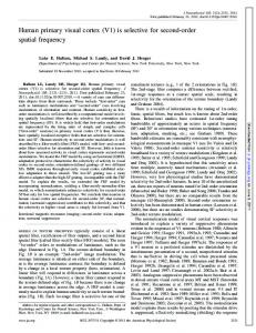
Figure 5. Orthogonal Dimensions of Visual Field Maps. Top Left: Eccentricity visual space legend. Each color represents an iso-eccentricity line in the left visual hemifield. Top Right: Polar angle visual space legend. Each color represents an iso-polar angle line in the left visual hemifield. (A) Eccentricity gradient for a visual field map (VFM). Note the gradient running from the center to more peripheral eccentricities runs from right to left. This gradient would be orthogonal to the polar angle gradient in (C), such that each isoeccentricity line has a representation of the full range of polar angles. (B) A VFM. The combination of the orthogonal gradients in (A) and (C) form one complete representation of a hemifield of visual space. This forms one half of a complete VFM, the corresponding half being located in the opposite hemisphere of the brain. Because the hemifield represented is the left, this map would be located in the right hemisphere. The black outer border indicates that each of the two gradients is located in the same portion of cortex. (C) Polar angle gradient for a VFM. Note that the colors of the cartoon in (C) are inverted with respect to the polar angle visual space legend at top. The inverted cartoon is meant to more accurately represent the inverted representation of visual space in early visual cortex. For example, in primary visual cortex (V1), the lower quarterfield of visual space is represented on the dorsal (upper) surface of the occipital lobe, and vice versa. (D) Two adjacent eccentricity gradients running in opposite directions, with adjacent representations of the central visual hemifield. (E) When the gradients in (D) are combined with adjacent polar angle gradients such as that in (F), two complete representations of the hemifield of visual space are formed. (F) Two adjacent polar angle gradients running in the same direction, with each iso-polar angle line for each gradient lying adjacent to one another. Note that if one only measured polar angle information, one would not have the corresponding eccentricity information to know whether that portion of cortex truly contained one (as in (B)), two (as in (E)), or more complete representations of that hemifield of visual space.


In addition to expert manual definition of VFMs, one can also use an automated tool to help give an objective definition of the boundary reversals between VFMs. Only a few of these tools are currently available, however. One such algorithm identifies VFMs by minimizing the error between an expected visual map (atlas) and the observed data [38]. In this tool, the atlas is coarsely aligned with the data and then elastically deformed. The search algorithm minimizes the weighted sum of deviations between the predicted and measured maps and the force of the elastic deformation. This algorithm is applied to both angle and eccentricity maps simultaneously to obtain a fit between these retinotopic measurements and templates of the two expected VFMs. This automated approach thus give more objective determinations of the boundaries of hemifield and quarter field visual angle representations or of the periphery edge of eccentricity representations, which can then be used to define specific VMFs. In cortical regions that have undetermined or ambiguous maps, this algorithm can be used to try a variety of possible templates of map organization (i.e., quarterfield map vs. hemifield map). Further, larger scale patterns of the organization of VFM across regions of cortex can be tested. By determining the error between the atlas template prediction and the actual angle and eccentricity measurements, the best fit template of VFM organization for a particular region can be estimated [11]. These atlas estimates can also be used to average map data across our subjects within a particular region of visual cortex [28]. The fitted atlas template additionally provides definitions of iso-angle and iso-eccentricity lines within each map, which can further be examined to compare patterns of VFM organization across the subject population [5, 11, 39].

3. Multiple visual field maps span human visual cortex This section will review current human VFM organization and some of the controversies surrounding these measurements.

3.1. Visual field maps in medial occipital cortex Three hemifield representations of visual space known as V1, V2, and V3 occupy the medial wall of occipital cortex in humans (Figures 2, 5, 6; for a review, see [12]). V1 is very reliably located in the calcarine sulcus, bounded on either side by the unique split-hemifield representations of V2 and V3 on the cuneus and lingual gyrus. V1 is known as “primary visual cortex,” because it receives direct input from the retino-geniculate pathway and is the first place in the retino-geniculo-cortical pathway where information from the two eyes is combined. Not only that, but V1 is an important site of basic calculations of orientation, color, and motion. Each computation is performed across the entire visual field, yet V1 appears at the level of fMRI measurements to be a single, smooth representation of visual space. One can think of V1 as several VFMs laid on top of one another, each of which performs a single computation (one overlapping map each for color, orientation, and motion). To accomplish this organization, a very intricate mosaic of neurons subserving these computations allows for each computation to be performed over each portion of visual space. These mosaics,


including ocular dominance columns, pinwheel orientation columns, and blobs/interblobs have been the subject of much study and argument (e.g., [2, 40, 41]). It remains to be seen how many maps throughout the visual hierarchy have similarly complex mosaics. V1, V2, and V3 each contain a foveal representation positioned at the occipital pole, with progressively more peripheral representations extending into more anteromedial cortex, forming complete eccentricity gradients (Figure 2; e.g., [12, 13, 15, 23]). The region where the individual foveal representations meet at the occipital pole is commonly referred to the as the foveal confluence [42]. Despite the apparent merging of these foveal representations into one confluent fovea in fMRI measurements of eccentricity gradients, distinct boundaries between V1, V2, and V3 have been shown to be present even within this most central foveal representation [42, 43].

Figure 6. Medial Occipital Cortex. The anatomical region containing early visual areas V1, V2, and V3 is shown within the black dotted circle on an inflated rendering of the cortical surface of a single left hemisphere from one subject. Gray represents sulci, and white represents gyri. Cu, cuneus; CaS, calcarine sulcus; LiG, lingual gyrus; POS, parieto-occipital sulcus; ColS, collateral sulcus.

The boundaries between each map are delineated by reversals in polar angle gradients (Figure 2, 5; e.g., [12, 13, 15, 23]). V1 has a contiguous polar angle gradient. In contrast, V2 and V3 have split-hemifield representations (quarterfields), which are denoted by their locations dorsal or ventral to V1 (V2d, V2v, V3d, V3v). For each map, the lower visual quarterfield is represented on the dorsal surface, and the upper visual quarterfield is represented on the ventral surface. The quarterfields of V2 and V3 are connected at the fovea for each map, but are otherwise distinct. Although some details differ between the macaque and human V1, V2, and V3 maps (for example, the surface area of macaque V1 is roughly half that of human V1), they are arguably the most similar between the species in terms of structure and function [14, 17, 19, 20, 44, 45]. Beyond these three maps, even as early as hV4, the anatomical and topographical details of the maps diverge [11, 46]. As a practical matter, due to their relatively consistent anatomical locations and unique concentric organization, these three maps form the first landmarks identified in visual field mapping analyses [10, 13]. However, as noted above, these three maps can differ


significantly in size across individuals. While V1 is always positioned along the calcarine sulcus in normal individuals, an increase in V1 size will necessarily shift the locations of V2 and V3 with respect to the specific underlying anatomy.

3.2. Visual field maps in ventral occipitotemporal cortex Beyond V3v, the organization of VFMs in human cortex no longer follows that of macaque. This divergence should not be surprising given that the two species diverged from a common ancestor approximately 25 million years ago [47]. While the fourth visual area of

Figure 7. Comparison of Human and Macaque Monkey Occipital Cortex. (A) 3D renderings of human (top) and macaque monkey (bottom) cortex are shown for a single right hemisphere. Cortical sheet is rendered at the white-gray boundary to allow visualization into the sulci. Hemispheres are scaled to relatively match in size. Scale bar is 1 cm. (B) Cartoon representations of flattened sections of cortex are centered on the occipital pole and show eccentricity gradients of human (top) and macaque (bottom) for visual field maps (VFMs) in posterior occipital cortex. Black lines denote boundaries between VFMs. Each color represents the location in visual space that best drives this region of cortex (see color legend inset for left visual field eccentricity). (C) Cartoon representations now show polar angle gradients of human (top) and macaque (bottom) for VFMs in posterior occipital cortex. Each color represents the location in visual space that best drives this region of cortex (see color legend inset for left visual field polar angle). Arrows (center) depict the approximate anatomical orientation for the cartoon representations in (B) and (C).


macaque remains a split-hemifield adjacent to area V3, human V4 (designated hV4 because of the unclear homology to macaque V4) is positioned as a complete hemifield on the ventral occipital surface adjacent to V3v (Figure 7). Several additional VFMs containing representations of complete, contiguous hemifields lie anterior to hV4 roughly along the fusiform gyrus (Figure 11). These maps are named and numbered for their anatomical locations: VO-1 and VO-2, for ventral-occipital, and PHC-1 and PHC-2, for parahippocampal cortex (Figure 8). The differences between human and macaque organization at the fourth visual area initially led to much controversy in the field regarding the organization of V4 in human, as some researchers sought a similar pattern of organization for the fourth visual area between human and macaque. To understand this controversy, it is important to review some of the history of measurements in this region. One of the early lines of investigation into the ventral surface focused on measurements of both color and retinotopic organization. Zeki and colleagues measured responses to an isoluminant pattern modulated in chromatic contrast in two regions of ventral occipitotemporal cortex: V4 and V4 alpha [48, 49]. McKeefry and Zeki [50] then demonstrated that the posterior color-responsive region of V4 was at least coarsely retinotopically organized and represented the entire contralateral hemifield. However, they did not locate this map with respect to other neighboring VFMs.

Figure 8. Ventral Occipitotemporal Cortex. The anatomical region containing ventral visual areas V2v, V3v, hV4, VO-1, VO-2, PHC-1, and PHC-2 is shown within the black dotted circle on an inflated rendering of the cortical surface of a single left hemisphere from one subject. CaS, calcarine sulcus; LiG, lingual gyrus; ColS, collateral sulcus; FuG, fusiform gyrus; PHG, parahippocampal gyrus. Other details as in Figure 6.

Hadjikhani et al. [51] also measured retinotopic and color organization along this region, describing two ventral retinotopic regions. The first was an upper quarterfield map, which they referred to as V4v. This putative V4v abutted the central visual field representation of V3v with an eccentricity map parallelingV1/V2/V3. Unlike the measurements of McKeefry and Zeki [50], they saw no adjacent lower quarterfield map that would form a complete contralateral hemifield. Instead, they described a hemifield map with an eccentricity representation that ran perpendicular to the putative V4v quarter field and called this VFM


V8. Using harmonic stimuli that alternated in luminance and chrominance, they also showed color responsivity within V8, although this stimulus type also would stimulate regions responsive to variations in luminance. Following the model of macaque cortex, Tootell and Hadjikhani [21] searched for a quarterfield map in dorsal occipital cortex to pair with their putative V4v. They failed to find the map and concluded that it did not exist. They did not resolve why an isolated quarterfield map would exist, a strange organization which would necessitate that whatever computation was subserved by putative V4v was only performed on one quarterfield of visual space. With improvements in measurement techniques, we clarified the retinotopic organization of this ventral region [11, 46]. Our experiments defined three VFMs in ventral occipital cortex: hV4, VO-1, and VO-2, which we showed to be involved in the color and object processing pathways. HV4 is a hemifield map on the posterior fusiform gyrus that directly abuts the upper hemifield representation of V3v and shares a common eccentricity orientation with the confluent foveal representations of V1, V2, and V3 (Figures 7, 8). Anterior to the peripheral representation of hV4 is a distinct group of VFMs with a shared foveal representation separate from that of V1, V2, V3, and hV4. We have termed this organization of a discrete group of VFMs a ‘clover leaf’ cluster, as described in more detail in Section 4 below. This ‘clover leaf’ cluster contains at least two full hemifield representations of visual space: VO-1 and VO-2. The posterior portion of VO-1 is adjacent to the relatively peripheral

visual field representation of hV4 and also abuts the peripheral V3v representation on the lingual gyrus. The posterior border of VO-1 represents the lower vertical meridian, and the anterior region represents the upper vertical meridian. This anterior upper vertical meridian reverses into the VO-2 hemifield map. The eccentricity gradient of VO-1 and VO-2 runs from the shared foveal representation on the fusiform gyrus anteromedially towards the more peripheral representation along the collateral sulcus and more anterior fusiform gyrus. Our recent measurements have suggested that additional maps (e.g., VO-3, VO-4) may be identified within this ‘clover leaf’ cluster in the future [52-54]. Our findings regarding hV4 and its neighbors have since been supported by measurements from several independent studies [28, 29, 39, 55-58]. Hansen et al. [57] initially continued the search for a hV4 organization more homologous to the split-hemifield of macaque V4 by proposing that a small section of dorsal lateral occipitotemporal cortex represented the inferior vertical meridian of hV4. This organization then left an hV4 division on the ventral surface that represented the full upper visual quarterfield adjacent to V3v plus some additional part of the visual field into the lower visual quarterfield. However, this organization conflicts with the now widely accepted dorsal occipitotemporal organization of LO-1 and LO-2 described below [28, 29, 39]. Further, additional measurements have now repeatedly confirmed 1) the full hemifield span of the ventral hV4 hemifield and 2) demonstrated that artifacts from a regional draining vein may in some subjects interfere with the accurate measurement of this section of hV4 [30]. Beyond hV4, VO-1, and VO-2, Arcaro et al. [55] defined two additional VFMs in this region that overlap with the parahippocampal place area, PHC-1 and PHC-2. Like the VFMs of the VO cluster, PHC-1 and PHC-2 also share a distinct foveal representation and appear in our


data to be two VFMs within another distinct ventral ‘clover leaf’ cluster [52]. PHC-1 is located just anterior to VO-2, running from the fusiform gyrus into the parahippocampal gyrus (Figure 8). Both PHC-1 and PHC-2 represent a full contralateral hemifield of visual space, with the representation of the upper vertical meridian denoting the boundary between PHC-1 and PHC-2.

3.3. Visual field maps in lateral occipitotemporal cortex In contrast to the posterior medial occipital VFMs, the lateral occipital cortex, with the object-responsive lateral occipital complex (LOC), has been much more difficult to measure in terms of retinotopic organization (Figure 9). This region was initially thought to be nonretinotopic or only to contain an ‘eccentricity bias’ (e.g., [21, 59, 60]). Recently, two VFMs, called LO-1 and LO-2 for ‘lateral occipital’, were described along the dorsal aspect of the LOC (Figure 11). LO-1 lies just anterior to V3d, reversing from the upper vertical meridian representation at the boundary into its representation of a full hemifield of visual space [28, 61]. LO-2 is located just inferior to LO-1, with the lower vertical meridian represented at the shared boundary of these two maps. The foveal representations of these two VFMs are located with the confluent foveal representations of V1, V2, V3, and hV4 on the occipital pole.

Figure 9. Lateral Occipitotemporal Cortex. The anatomical region containing lateral visual areas LO-1, LO-2, and the hMT+ cluster is shown within the black dotted circle on an inflated rendering of the cortical surface of a single left hemisphere from one subject. STS, superior temporal sulcus; ITS, inferior temporal sulcus; LOG, lateral occipital gyri; AnG, angular gyrus; IPS, intraparietal sulcus; TOS, transverse occipital sulcus; OP, occipital pole. Other details as in Figure 6.

In addition, regions just inferior to these maps have been shown to be responsive to lateralized visual stimuli, but have not yet been divided into specific VFMs [27, 62-64]. In


macaque, there has been increasing electrophysiological evidence that neurons in homologous regions may maintain a high degree of retinotopic sensitivity [65]. It is important to note again that the presence of organized representations of visual space in this region can still allow for the stimulus size and position invariance frequently described across the objectresponsive LOC. PRF sizes are expected to be large across this region, but may maintain just enough dispersion of pRF centers to allow for slightly different preferred tuning of responses to visual space. Thus, the responses to object stimuli from this cluster could remain both invariant to stimulus size and position over a wide field of view while retaining visuospatial information. With LO-1 and LO-2, the definition of additional VFMs spanning LOC would form the lateral half of an occipital pole ‘clover leaf’ cluster and would provide a concrete, visuospatial framework for reliably localizing specific computational regions within lateral object-responsive cortex [5, 12, 66, 67]. This inferior region of the LOC merges with the most lateral lower vertical meridian representation of hV4 [11] and is also subject to issues with the ‘venous eclipse’ fMRI artifact due to the presence of a draining vein here that has a somewhat variable position across subjects within this region [30]. This artifact has likely significantly contributed to the difficulties in measuring organized VFMs within this region. Anterior to LOC, along the banks of the inferior temporal sulcus, lies the TO cluster, also known as hMT+ (Figure 9). Amano et al. [29] were able to provide the first clear measurements of VFMs in the human motion-selective MT complex (hMT+) using the pRF methods described above [68]. They named these two new hemifield VFMs TO-1 and TO-2, for temporal-occipital areas 1 and 2. These maps are positioned just anterior to the LO maps and share another distinct foveal representation. The representations of visual of space across these maps run anteriorly from the lower vertical meridian at the posterior border of TO-1, to the shared upper vertical meridian at the border of TO-1 and TO-2, to the lower vertical meridian at the anterior border. Following measurements by Huk et al. [68] that demonstrated retinotopic organization within the MT subdivision and differentiated human MT and human MST using dissociable motion stimuli, it is likely that TO-1 is the same as human MT, and TO-2 is the same as human MST. Recently, Kolster et al. [39] verified that both TO-1 and TO-2 represent full, organized hemifields of visual space, but used a naming scheme homologous to macaque with MT and ‘putative’ MST (pMST). They also expanded the VFM measurements of this region, showing that the TO/hMT+ cluster contains four full hemifields of visual space. The two additional hemifields of visual space merge at the confluent fovea of TO-1 and TO-2 and are located just inferior to TO-1 and TO-2. They suggest that these VFMs correspond to macaque FST and V4t. Human ‘putative’ FST (pFST) is positioned anterior to human ‘putative’ V4t (pV4t), and the two VFMs meet an upper vertical meridian representation. Around this cluster, MT/V5 (TO-1) then shares a lower vertical meridian border with pV4t, and pMST (TO-2) shares a lower vertical meridian border with pFST. A similar clustered organization of these motion responsive VFMs in macaque has also recently been demonstrated by Kolster et al. [69]. We confirm these measurements with data showing the ‘clover leaf’ cluster organization for this group of VFMs in the human MT+ complex [5, 11, 12, 66, 67]. Because the homology to monkey has not yet been verified, we prefer the anatomy-based


terminology TO-1, TO-2, TO-3, and TO-4 for these VFMs; these would correspond to Kolster et al.’s [39] MT, pMST, pFST, and pV4t, respectively. Amano et al. [29] and Kolster et al. [39] disagreed, however, on the specific organization of the eccentricity gradients between the LO VFMs and the TO/hMT+ VFMs [29, 39]. Amano et al. [29] described LO-2 and TO-1 as positioned as a strip of VFMs on the lateral occipital surface, with hemifield representations sharing meridian boundaries from V3d, to LO-1, to LO-2, to TO-1, to TO-2. In this organization, LO-2 and TO-1 would share a boundary that represents the lower vertical meridian. TO-1 and TO-2 would still meet at a discrete foveal representation that runs only from the foveal representation to a more superior peripheral representation that merges only superiorly with that of LO-2. In contrast, Kolster et al. [39] describe the TO maps as a distinct cluster anterior to LOC and the LO maps, which do not share any meridian boundaries. With this cluster organization, it is the peripheral representation that is shared between the LO and TO maps. Our measurements confirm those of Kolster et al. [5, 11, 39, 66, 67]. The four TO maps form a complete ‘clover leaf’ cluster that merges with the eccentricity gradients of the LO VFMs at their peripheral eccentricity representations. This VFM definition can be seen in the data in Figure 1 of Amano et al. [29], but was differently interpreted prior to the measurements of the full TO ‘clover leaf’ cluster. Finally, Kolster et al. [39] describe an additional putative new cluster of two VFMs inferior to the TO/hMT cluster they term putative human PIT (phPIT) based on possible homology to macaque PIT [39]. These are the first measurements of these VFMs in human and have not yet been verified by other labs. As techniques improve and we learn more about the effects of the venous eclipse artifact in this region [30], we expect that multiple VFMs will be measured by multiple labs in this and surrounding regions in future measurements [53, 66, 67].

3.4. Visual field maps in posterior parietal cortex Beyond the medial part of the dorsal lower vertical meridian representation of human V3d, lies a series of hemifield VFMs running from the transverse occipital sulcus (TOS) up along the medial wall of the intraparietal sulcus (IPS) (Figures 10, 11; e.g., [12, 70]). The first maps bordering V3d are V3A and V3B [71-73]. These two maps share another discrete foveal representation within the TOS, forming a complete ‘clover leaf’ cluster [5]. V3A has some similarities to macaque V3A and is thought to play a role in motion processing; the computations subserved by V3B are not yet known [71, 72, 74, 75]. V3B was originally described Smith et al. [72] as at least a quarterfield of visual space next to V3A. This definition was expanded to cover a while hemifield of visual space by Press et al. [71], who noted that this region of V3A had a full hemifield polar angle gradient with an eccentricity gradient expanding concentrically from a central position within this hemifield. Such an organization necessitates that two representations of visual space are represented; thus, V3A and V3B were described in Press et al. [71]as a cluster of two VFMs sharing a distinct fovea. In comparing the initial V3B definitions from Smith et al. [72] and later definitions of LO-1 [2729], which is just lateral and inferior to V3B, it is possible that the original V3B definitions were measuring a part of what was later called LO-1 and not the same hemifield that was described in Press et al. [71] as V3B. The field now generally considers V3A and V3B as the cluster of two VFMs in the TOS, and LO-1 and LO-2 as the dorsal aspect of the LO [12, 27-29].


Figure 10. Posterior Parietal Cortex. The anatomical region containing dorsal posterior parietal cortex visual areas V3A, V3B, and the IPS maps is shown within the black dotted circle on an inflated rendering of the cortical surface of a single left hemisphere from one subject. STS, superior temporal sulcus; IPS, intraparietal sulcus; POS, parieto-occipital sulcus; TOS, transverse occipital sulcus; OP, occipital pole. Other details as in Figure 6.

Entering into the IPS, the next VFM anterior to the V3A/V3B cluster is IPS-0 (formerly called V7) [75, 76]. IPS-0 has a foveal representation distinct from the V3A/V3B cluster and represents a full hemifield of contralateral visual space, running from the lower vertical meridian representation at the posterior border to the upper vertical meridian representation anteriorly. Beyond IPS-0, a series of polar angle representations extends from IPS-0 along the medial wall of the IPS. All these polar angler representations have been primarily measured using attentionally demanding traveling wave stimuli, consistent with the description of this parietal region as having a role in spatial attention [74-79]. These representations have primarily been described as reversing smoothly through a strip of several hemifield representations from IPS-0 to IPS-5 [70, 76-78, 80-82]. It is important here to differentiate “polar angle representations” from complete “VFMs.” For the initial part of the IPS, VFM IPS-0 (V7) has been relatively well characterized [76, 83]. However, VFMs IPS-1 through IPS-5 as well as human LIP (a possible homologous region to macaque LIP which has been suggested to align with IPS-1 or IPS-2) have been exclusively presented in the literature to date as only polar angle maps [70, 76-82, 84, 85], except for the one example we have found of an eccentricity representation in two hemispheres of one subject (see Figure 4 in [81]). Swisher et al. [81] note, for example, that “we reliably find a continuous gradient of eccentricity response phase along the V7(IPS-0)/ IPS-1 border,” but that “the eccentricity representation in IPS-3/4 is less clear.” Some of these studies have reported that eccentricity mapping was used in the VFM definitions, but failed to our


knowledge, with the one exception, to show anything but the polar angle responses in the published data (main or supplemental).

Figure 11. The Current State of Contiguous Visual Field Maps in Occipital, Parietal, and Temporal Lobes of Human Cortex. The figure depicts a cartoon overview of hemifield representations of visual field maps (VFMs) in a single right hemisphere if the cortical sheet of that hemisphere were removed from its usual position and laid flat. The center of the blue region is centered on the occipital pole, while the purple region is in parietal cortex, the red and yellow regions are on the ventral surface of the occipital and temporal lobes, and the green region is on the lateral surface of the temporal lobe. Each color except purple represents a likely or confirmed ‘clover leaf’ cluster of VFMs. Solid black lines indicate the borders between ‘clover leaf’ clusters and dotted lines indicate the borders between hemifield representations within clusters. In the purple region, the organization is much less clear, particularly for maps outlined in dotted rather than solid black lines (IPS-1, IPS-2, IPS-3, IPS-4, IPS-5, SPL1, and V6A). See main text for more details.


While polar angle representations (i.e., IPS-1/2/3/4/5) are excellent indicators that one or a number of VFMs may exist in a given location, they do not provide evidence of a unique, complete VFM. In the case of the IPS polar angle gradients, there could be any number of reversals of eccentricity representations along the polar iso-angle lines. Without obtaining clear, reliable orthogonal maps of both dimensions, it is impossible to know exactly how to divide up a region into multiple representations of visual space. We encountered such a division of what had appeared to be a single hemifield polar angle represenation into multiple VFMs given a central foveal representation previously in the segregation of human V3A into the 2-map cluster with V3B [71]. In those measurements, what had appeared to simply be a large single hemifield representation of V3A, we showed to actually be divided into two full hemifield maps of visual space along the centrally positioned foveal representation [5]. Current work is suggesting that the parietal cortex anterior to the V3A/V3B cluster may also in fact contain several additional ‘clover leaf’ clusters with VFMs that share several confluent, discrete foveae along the IPS [86, 87]. The medial wall of the parietal lobe has also been shown to contain at least three additional retinotopically organized regions. One VFM called V6 lies along the parieto-occipital sulcus just anterior to the peripheral representation of V3d [88, 89]. V6 represents the contralateral hemifield, with an inferior upper vertical meridian running superiorly to the lower vertical meridian representation and a distinct eccentricity gradient that extends far into the periphery. V6 has been shown to be involved in particular types of motion processing, such as pattern and self motion [89]. Adjacent to V6 is another VFM termed V6A [88-90]. Both areas are named to represent their expected homology to macaque. Human V6A has primarily been measured using visual stimuli that activate the far periphery and is likely involved in visuomotor integration [88, 89]. V6A contains at least a coarse representation of the contralateral hemifield and a very peripheral eccentricity gradient with expansion the representation of > 35° visual angle. The last retinotopic region so far measured here is named SPL1 (for superior parietal lobule 1) and is located just medial to the series of maps running along the IPS [70, 82, 85]. Although its position appears somewhat variable across subjects and publications with respect to the specific IPS maps it borders, it appears to be primarily located adjacent to IPS-2, IPS-3 and/or IPS-4. The polar angle gradient of SPL1 runs from its lower vertical meridian border along these IPS maps inferiorly to its upper vertical meridian border. To our knowledge, no eccentricity gradients for this region have yet been demonstrated in the literature. Like the other maps along the IPS, SPL1 may also play a role in spatial attention.

3.5. Visual field maps in frontal cortex Several topographically organized representations of the contralateral hemifield have also been demonstrated in frontal cortex by a few studies using a variety of stimuli including TWR, visual spatial attention tasks, and memory-guided saccade tasks [70, 78, 79, 84, 85, 91]. These topographic representations of the polar angle of visual space arise in the frontal eye fields (FEF), the supplementary eye fields (SEF), dorsolateral prefrontal cortex (DLPFC), and precentral cortex (pre-CC), regions involved in complex visual processing of spatial


attention and eye movement control (Figure 12). Like many of the measurements shown for the IPS region, these frontal regions also lack measurements of orthogonal eccentricity representations. It remains to be seen whether these attentional regions contain only very coarse eccentricity gradients that is difficult to measure or whether future measurements will unveil more detailed eccentricity gradients and possibly multiple VFMs within each topographic region.

Figure 12. Frontal Cortex.SFS, superior frontal sulcus; IFS, inferior frontal sulcus; PreCS, precentral sulcus; CS, central sulcus; LF, lateral fissure. Other details as in Figure 6.

It is important to note that the stimulus paradigms used to define these regions do not differentiate between retina-centered (retinotopic) and head-, gaze-, body-, or worldcentered (spatiotopic) topographic organization. While the VFMs in the occipital lobe have been shown to be retinotopically organized [92], there is more controversy regarding if and where the visual system transforms from retinotopic to spatiotopic organization. Spatiotopic representations have been suggested to be present in some visuo-motor pathways (for review, see [93]), but have also been shown to not be necessary for such transformations [94]. Similarly, the native coordinate system of spatial attention has been shown to be retinotopic [95, 96], suggesting that retina-centered visuospatial information is propagated throughout the visual system.

4. Organizational patterns of visual field maps across human cortex As increasing numbers of VFMs have been defined in human visual cortex, one question that has arisen is whether there is an organizing principle for the distribution of these maps across visual cortex [5, 11, 58, 60, 69, 97, 98]. A basic approach that has worked for early visual cortex has been to define strings of VFMs along contiguous strips of occipital cortex, with adjacent portions of the maps representing similar portions of visual space, but performing different computations [3]. This configuration of maps again allows for more efficient connections between neurons in different maps, such that for a given portion of


space, the length of the axons between neurons performing different sets of computations in the process of building the visual percept is minimized [6, 7, 99]. As additional VFMs have been defined in higher order visual cortex, more complex organizing principles for visual cortex have been proposed [5, 11, 58, 60, 69, 97, 98, 100, 101]. One such principle describes VFMs as organized into roughly circular clusters that we have termed ‘clover leaf clusters’ (Figure 13) [5, 11, 66, 67]. These clusters are hypothesized to each contain multiple VFMs which share similar processing properties across that cluster [5, 11, 69]. Several clusters have been partially described, and two have been repeatedly mapped in full: V3A/V3B and TO/hMT+ clusters [5, 11, 12, 29, 39].

Figure 13. Orthogonal Dimensions of ‘Clover Leaf’ Clusters. Top Left: Eccentricity visual space legend. Each color represents an iso-eccentricity line in the left visual hemifield. Top Right: Polar angle visual space legend. Each color represents an iso-polar angle line in the left visual hemifield. (A) Eccentricity gradients of a typical ‘clover leaf’ cluster, containing 4 complete representations of the left visual hemifield. Each eccentricity gradient from the center to periphery of visual space runs physically from the center to the periphery of the cluster, such that iso-eccentricity lines form concentric circles about the center of the cluster. (B) A typical ‘clover leaf’ cluster with 4 complete representations of a hemifield of visual space. Note that, due to the radially orthogonal organization of ‘clover leaf’ clusters, each individual map must be shaped like a piece of pie. (C) Polar angle gradients of a typical ‘clover leaf’ cluster. Each iso-polar angle line runs from the center to periphery of the cluster like a ‘spoke of the wheel’ of the cluster, such that each polar angle gradient runs from one ‘spoke of the wheel’ of the cluster around to another ‘spoke’. Note that, due to the fact that polar angle reversals (adjacent spokes with the same polar angle preference) denote the boundaries between hemifield representations within a ‘clover leaf’ cluster, there must always be an even number of hemifield representations in each ‘clover leaf’ cluster. To have an odd number would necessarily require a discrete jump in polar angle representation between hemifield representations, which has so far not been observed in human visual field mapping.

The VFMs within a ‘clover leaf’ clusters are organized such that the central fovea is represented in the center of the cluster, with more peripheral representations of space represented in more peripheral positions in the cluster in a smooth, orderly fashion. The representation of any given polar angle of space for any given VFM extends out from the


center to the periphery of the cluster, effectively spanning the radius of the cluster like a spoke on a wheel. We refer to this type of organization – one dimension of space (polar angle) represented radially from center to periphery of a cluster and the other dimension (eccentricity) represented in concentric, circular bands from center to periphery – as being radially orthogonal. Furthermore, we expect that these clusters have consistent locations relative to one another, but that the maps within each cluster may be oriented somewhat differently. Finally, VFMs within each ‘clover leaf’ clusters are proposed to perform similar types of computations. This broad scale organizational pattern of VFM is currently under investigation by several groups [5, 7, 12, 39, 66, 67, 69], and we expect it to extend across human visual cortex.

5. Additional measurements to refine human visual field map definitions 5.1. White matter connectivity among human visual field maps In order to fully investigate visuospatial processing in the human brain, it is important to measure not only patterns of functional VFM organization across cerebral cortex, but also the organization of the white matter tracts connecting these functional regions. Feedforward and feedback information from each VFM must be passed on to other maps up and down the hierarchy of visual processing [18]. The retinotopic human visual system processes portions of visual space in parallel, requiring connections for one type of processing in any particular location of the visual field to be passed to the same location of visual space in the next VFM for the next step in visual processing [102]. An elegant solution to this connectivity problem would be to maintain visuospatial organization in the white matter tracts between clusters. Such a solution allows for molecular cues to guide and maintain the relative structure of VFMs. Any other solution would necessarily require a breakdown of

Figure 14. White matter connections in human visual cortex. (a) An example of separate sets of diffusion tensor imaging fibers estimated among maps in parietal cortex. Fibers originated from a 5 mm seed point located in the dorsal polar angle gradients IPS-1. Fibers colored red illustrate intrahemispheric U-fibers connecting neighboring locations in left intraparietal sulcus (IPS). Blue and green fibers depict 2 subsets of a group of inter-hemispheric fiber tracks that connect to the contralateral IPS.


the organization inherent in connections coming out of a cluster into some other organization, and a rebuilding of the organization inherent in connections going into the next cluster, which is more costly, difficult, and complicated. The MR protocol of diffusion tensor imaging (DTI) is beginning to provide such measurements of connectivity among VFMs early in the visual processing hierarchy (Figure 14). DTI is based upon a computer-assisted analysis of multiple diffusion-weighted images and uses a Gaussian model of diffusion, called an ellipsoid or ‘tensor’, to measure the mobility of water molecules within human tissue [103]. Traditional DTI measurements include fractional anisotropy (FA) and mean diffusivity (MD); custom software packages allow one to now also estimate the shapes, properties and destinations of white matter fiber tracts from DTI data (e.g., [104, 105]; http://white.stanford.edu/software/). The combination of DTI and fiber-tracking algorithms that combine tensors with similar principal diffusion directions can produce estimates of the major fiber bundles in the brain of individual subjects [106, 107]. FA, MD, and estimated fiber track locations and densities can be compared across individuals and between groups of subjects [108]. DTI has now successfully been used to measure the organization of the human optic tracts and optic radiations from the retina to the LGN to V1 [50, 109]. These measurements of the initial visual tracts match those measured by other methods [12, 110] and are now being used in studies examining how the optic radiations differ in specific patient populations (e.g., [32]). In cortex, DTI measurements have further demonstrated that the retinotopic organization of V1 is maintained in connections between homologous VFMs across hemispheres, with upper and lower visual field sections running together through the splenium of the corpus callosum [108, 111, 112]. These emerging measurements of white matter connectivity among VFMs will aid us both in refining our definitions of specific VFM boundaries throughout the visual processing hierarchy, especially in regions with more ambiguous VFM measurements, and in expanding our understanding of specific computational pathways.

5.2. Integration of visual field maps with other functional measurements in human visual cortex The findings from combined structural and functional measurements have a profound impact on the study of vision in the brain. Any visual area that is organized retinotopically is subject to the constraints common to all VFMs in the human brain. Many areas of the brain have been considered “non-retinotopic” or containing only an “eccentricity bias,” because laboratories using the field standard TWR were not able to demonstrate complete, precise retinotopic organization (e.g., [21, 97, 113]). Typically, this has been interpreted to mean that the early portion of the visual system is the only part that is retinotopic, and, at some point midway in the hierarchy, there must be a fundamental change in the way that the visual system is constructed. Not only is this a major theoretical claim, which would require a potentially complex transformation from a retinotopic framework to some other non-spatial organization, but it side-steps the basic fact that properties such as retinal-size-


invariant object recognition can occur in VFMs without any cost. It is possible that the majority of higher order visual areas are retinotopic, maintaining retinotopically organized, dispersed receptive field centers despite increasingly large receptive field sizes. Why would we evolve an entirely different way to deal with one type of visual information when the simple solution of using large receptive fields and population codes within VFMs does not require a change in organization or connectivity? We contend that any failure to demonstrate retinotopic responses in a visually responsive area must be first carefully evaluated as a failure of the measurement methodology. This is a question whose answer is vital to understanding higher-order cognition, which need not abandon the visuospatial knowledge gained from low-level visual processing.

6. Conclusion Our understanding the visuospatial organization of human visual cortex is crucial for our further exploration of the computations subserved by these visual pathways. Because every human brain shares common functional topography that is somewhat variably located anatomically, it is vital to correctly localize common functional areas in individual subjects in order to then study which specific computations are carried out by each area. The widespread technique of mapping anatomy to a common atlas not only destroys information about individual subjects, but also blurs data from adjacent areas within each subject, making it impossible to differentiate computations in adjacent areas. This chapter has reviewed the primary measurement techniques for investigating the organization of human visual cortex as well as the present state of knowledge of the visuospatial representations across cortex. Until recently, the best technique for localizing visual field maps was TWR, which is excellent at identifying the centers of pRFs in fMRI voxels. Now, that technique has been surpassed by pRF modeling, which measures not only pRF centers, but the spread of each pRF. Both techniques have been used to successfully localize numerous visual field maps, most of which have been confirmed by numerous laboratories. However, it would be a mistake to assume that the current organizational model is entirely correct or complete. Some polar angle gradients still need to have eccentricity gradients measured in order to correctly determine the number of VFMs in parts of cortex such as posterior parietal cortex. Other maps simply need confirmation in the form of replication by independent laboratories. Perhaps most importantly, the current organizational model will need to be reconsidered in the face of evidence that VFMs are organized into ‘clover leaf’ clusters. These data will surely be updated as additional measurements both expand the known retinotopic representations in human visual cortex and clarify the current VFM definitions.

Author details Alyssa A. Brewer and Brian Barton Department of Cognitive Sciences, University of California, Irvine, USA


Acknowledgement This work was supported by University of California, Irvine, startup funds to A.A.B.

7. References [1] W. H. Merigan and J. H. Maunsell, "How parallel are the primate visual pathways?," Annu Rev Neurosci, vol. 16, pp. 369-402, 1993. [2] D. L. Adams, L. C. Sincich, and J. C. Horton, "Complete pattern of ocular dominance columns in human primary visual cortex," J Neurosci, vol. 27, pp. 10391-403, Sep 26 2007. [3] B. A. Wandell, S. O. Dumoulin, and A. A. Brewer, "Visual cortex in humans," in Encyclopedia of Neuroscience. vol. 10, L. R. Squire, Ed., ed Oxford: Academic Press, 2009, pp. 251-257. [4] J. H. Kaas, "Topographic Maps are Fundamental to Sensory Processing," Brain Research Bulletin, vol. 44, pp. 107–112, 1997. [5] B. A. Wandell, A. A. Brewer, and R. F. Dougherty, "Visual field map clusters in human cortex," Philos Trans R Soc Lond B Biol Sci, vol. 360, pp. 693-707, Apr 29 2005. [6] G. Mitchison, "Neuronal branching patterns and the economy of cortical wiring," Proc Biol Sci, vol. 245, pp. 151-8, Aug 22 1991. [7] D. B. Chklovskii and A. A. Koulakov, "Maps in the brain: what can we learn from them?," Annu Rev Neurosci, vol. 27, pp. 369-92, 2004. [8] R. Shapley, M. Hawken, and D. Xing, "The dynamics of visual responses in the primary visual cortex," Prog Brain Res, vol. 165, pp. 21-32, 2007. [9] F. Moradi and D. J. Heeger, "Inter-ocular contrast normalization in human visual cortex," J Vis, vol. 9, pp. 13 1-22, 2009. [10] S. A. Engel, D. E. Rumelhart, B. A. Wandell, A. T. Lee, G. H. Glover, E. J. Chichilnisky, and M. N. Shadlen, "fMRI of human visual cortex," Nature, vol. 369, p. 525, Jun 16 1994. [11] A. A. Brewer, J. Liu, A. R. Wade, and B. A. Wandell, "Visual field maps and stimulus selectivity in human ventral occipital cortex," Nat Neurosci, vol. 8, pp. 1102-9, Aug 2005. [12] B. A. Wandell, S. O. Dumoulin, and A. A. Brewer, "Visual field maps in human cortex," Neuron, vol. 56, pp. 366-83, Oct 25 2007. [13] M. I. Sereno, A. M. Dale, J. B. Reppas, K. K. Kwong, J. W. Belliveau, T. J. Brady, B. R. Rosen, and R. B. Tootell, "Borders of multiple visual areas in humans revealed by functional magnetic resonance imaging," Science, vol. 268, pp. 889-93., 1995. [14] D. C. Van Essen, J. W. Lewis, H. A. Drury, N. Hadjikhani, R. B. Tootell, M. Bakircioglu, and M. I. Miller, "Mapping visual cortex in monkeys and humans using surface-based atlases," Vision Res, vol. 41, pp. 1359-78, 2001. [15] E. A. DeYoe, G. J. Carman, P. Bandettini, S. Glickman, J. Wieser, R. Cox, D. Miller, and J. Neitz, "Mapping striate and extrastriate visual areas in human cerebral cortex," Proc Natl Acad Sci U S A, vol. 93, pp. 2382-6, Mar 19 1996. [16] D. C. Van Essen, "Behind the optic nerve: an inside view of the primate visual system," Trans Am Ophthalmol Soc, vol. 93, pp. 123-33, 1995.


[17] D. C. Van Essen, W. T. Newsome, and J. H. Maunsell, "The visual field representation in striate cortex of the macaque monkey: asymmetries, anisotropies, and individual variability," Vision Res, vol. 24, pp. 429-48, 1984. [18] D. J. Felleman and D. C. V. Essen, "Distributed hierarchical processing in the primate cerebral cortex," Cerebral Cortex, vol. 1, pp. 1-47, 1991. [19] D. C. Van Essen, Organization of visual areas in macaque and human cerebral cortex. Boston: Bradford, 2003. [20] D. C. Van Essen, D. J. Felleman, E. A. DeYoe, J. Olavarria, and J. Knierim, "Modular and hierarchical organization of extrastriate visual cortex in the macaque monkey," Cold Spring Harb Symp Quant Biol, vol. 55, pp. 679-96, 1990. [21] R. B. Tootell and N. Hadjikhani, "Where is 'dorsal V4' in human visual cortex? Retinotopic, topographic and functional evidence," Cereb Cortex, vol. 11, pp. 298-311, Apr 2001. [22] S. O. Dumoulin and B. A. Wandell, "Population receptive field estimates in human visual cortex," Neuroimage, vol. 39, pp. 647-60, Jan 15 2008. [23] S. A. Engel, G. H. Glover, and B. A. Wandell, "Retinotopic organization in human visual cortex and the spatial precision of functional MRI," Cereb Cortex, vol. 7, pp. 181-92, Mar 1997. [24] E. A. DeYoe, G. J. Carman, P. Bandettini, S. Glickman, J. Wieser, R. Cox, D. Miller, and J. Neitz, "Mapping striate and extrastriate visual areas in human cerebral cortex," Proc. Natl. Acad. Sci. (USA), vol. 93, pp. 2382-2386, 1996. [25] M. I. Sereno, C. T. McDonald, and J. M. Allman, "Analysis of retinotopic maps in extrastriate cortex," Cerebral Cortex, vol. 6, pp. 601-620, 1994. [26] B. A. Wandell and J. Winawer, "Imaging retinotopic maps in the human brain," Vision Res, vol. 51, pp. 718-37, Apr 13 2011. [27] R. Sayres and K. Grill-Spector, "Relating retinotopic and object-selective responses in human lateral occipital cortex," J Neurophysiol, vol. 100, pp. 249-67, Jul 2008. [28] J. Larsson and D. J. Heeger, "Two retinotopic visual areas in human lateral occipital cortex," J Neurosci, vol. 26, pp. 13128-42, Dec 20 2006. [29] K. Amano, B. A. Wandell, and S. O. Dumoulin, "Visual field maps, population receptive field sizes, and visual field coverage in the human MT+ complex," J Neurophysiol, vol. 102, pp. 2704-18, Nov 2009. [30] J. Winawer, H. Horiguchi, R. A. Sayres, K. Amano, and B. A. Wandell, "Mapping hV4 and ventral occipital cortex: the venous eclipse," J Vis, vol. 10, p. 1, 2010. [31] S. Prakash, S. O. Dumoulin, N. Fischbein, B. A. Wandell, and Y. J. Liao, "Congenital achiasma and see-saw nystagmus in VACTERL syndrome," J Neuroophthalmol, vol. 30, pp. 45-8, Mar 2010. [32] N. Levin, S. O. Dumoulin, J. Winawer, R. F. Dougherty, and B. A. Wandell, "Cortical maps and white matter tracts following long period of visual deprivation and retinal image restoration," Neuron, vol. 65, pp. 21-31, Jan 14 2010. [33] H. A. Baseler, A. Gouws, K. V. Haak, C. Racey, M. D. Crossland, A. Tufail, G. S. Rubin, F. W. Cornelissen, and A. B. Morland, "Large-scale remapping of visual cortex is absent


[34]

[35] [36]

[37] [38]

[39]

[40]

[41] [42] [43]

[44] [45]

[46]

[47] [48]

in adult humans with macular degeneration," Nat Neurosci, vol. 14, pp. 649-55, May 2011. F. Maes, A. Collignon, D. Vandermeulen, G. Marchal, and P. Suetens, "Multimodality image registration by maximization of mutual information," IEEE Trans Med Imaging, vol. 16, pp. 187-98, Apr 1997. B. A. Wandell, S. Chial, and B. T. Backus, "Visualization and measurement of the cortical surface," J Cogn Neurosci, vol. 12, pp. 739-52, Sep 2000. P. C. Teo, G. Sapiro, and B. A. Wandell, "Creating connected representations of cortical gray matter for functional MRI visualization," IEEE Trans Med Imaging, vol. 16, pp. 85263, Dec 1997. O. Nestares and D. J. Heeger, "Robust multiresolution alignment of MRI brain volumes," Magn Reson Med, vol. 43, pp. 705-15, May 2000. R. F. Dougherty, V. M. Koch, A. A. Brewer, B. Fischer, J. Modersitzki, and B. A. Wandell, "Visual field representations and locations of visual areas V1/2/3 in human visual cortex," J Vis, vol. 3, pp. 586-98, 2003. H. Kolster, R. Peeters, and G. A. Orban, "The retinotopic organization of the human middle temporal area MT/V5 and its cortical neighbors," J Neurosci, vol. 30, pp. 9801-20, Jul 21 2010. E. Bartfeld and A. Grinvald, "Relationships between orientation-preference pinwheels, cytochrome oxidase blobs, and ocular-dominance columns in primate striate cortex," Proc Natl Acad Sci U S A, vol. 89, pp. 11905-9, Dec 15 1992. M. S. Livingstone and D. H. Hubel, "Anatomy and physiology of a color system in the primate visual cortex," J Neurosci, vol. 4, pp. 309-56, Jan 1984. M. M. Schira, C. W. Tyler, M. Breakspear, and B. Spehar, "The foveal confluence in human visual cortex," J Neurosci, vol. 29, pp. 9050-8, Jul 15 2009. M. M. Schira, C. W. Tyler, B. Spehar, and M. Breakspear, "Modeling magnification and anisotropy in the primate foveal confluence," PLoS Comput Biol, vol. 6, p. e1000651, Jan 2010. M. G. Rosa, "Visuotopic organisation of primate extrastriate cortex.," in Cerebral Cortex. vol. 12, K. J. Rockland KS, Peters A, Ed., ed New York: Plenum Press, 1997, pp. 127–203. M. G. Rosa and R. Tweedale, "Brain maps, great and small: lessons from comparative studies of primate visual cortical organization," Philos Trans R Soc Lond B Biol Sci, vol. 360, pp. 665-91, Apr 29 2005. A. R. Wade, A. A. Brewer, J. W. Rieger, and B. A. Wandell, "Functional measurements of human ventral occipital cortex: retinotopy and colour," Philos Trans R Soc Lond B Biol Sci, vol. 357, pp. 963-73, Aug 29 2002. S. B. Hedges and S. Kumar, "Genomic clocks and evolutionary timescales," Trends in Genetics, vol. 19, pp. 200-206, 2003. C. J. Lueck, S. Zeki, K. J. Friston, M.-P. Deiber, P. Cope, V. J. Cunningham, A. A. Lammertsma, C. Kennard, and R. S. J. Frackowiak, "The color center in the cerebral cortex of man," Nature, vol. 340, pp. 386-389, 1989.


[49] S. Zeki, J. D. G. Watson, C. J. Lueck, K. J. Friston, C. Kennard, and R. S. J. Frackowiak, "A direct demonstration of functional specialization in human visual cortex.," J. Neuroscience, vol. 11, pp. 641-649, 1991. [50] D. J. McKeefry and S. Zeki, "The position and topography of the human colour centre as revealed by functional magnetic resonance imaging," Brain, vol. 120, pp. 2229-42, 1997. [51] N. Hadjikhani, A. K. Liu, A. M. Dale, P. Cavanagh, and R. B. Tootell, "Retinotopy and color sensitivity in human visual cortical area V8," Nat Neurosci, vol. 1, pp. 235-41, Jul 1998. [52] S. A. Drew, D. E. Asher, B. Barton, and A. A. Brewer, "Pinwheel cartography: New visual field map cluster in the human posterior parahippocampal complex," presented at the Society for Neuroscience, San Diego, CA, 2010. [53] D. E. Asher and A. A. Brewer, "Hemispheric differences of color responses in human ventral visual cortex," Vision Sciences Society. Journal of Vision, vol. 9, pp. 776-776, 2009. [54] D. E. Asher, S. A. Drew, B. Barton, and A. A. Brewer, "Pinwheel cartography: Novel visual field map cluster within human ventro-lateral occipital cortex. ," presented at the Society for Neuroscience, San Diego, CA, 2010. [55] M. J. Arcaro, S. A. McMains, B. D. Singer, and S. Kastner, "Retinotopic organization of human ventral visual cortex," J Neurosci, vol. 29, pp. 10638-52, Aug 26 2009. [56] S. Kastner, P. De Weerd, M. A. Pinsk, M. I. Elizondo, R. Desimone, and L. G. Ungerleider, "Modulation of sensory suppression: implications for receptive field sizes in the human visual cortex," J Neurophysiol, vol. 86, pp. 1398-411, Sep 2001. [57] K. A. Hansen, K. N. Kay, and J. L. Gallant, "Topographic organization in and near human visual area V4," J Neurosci, vol. 27, pp. 11896-911, Oct 31 2007. [58] C. W. Tyler and A. R. Wade, "Extended concepts of occipital retinotopy," Current Medical Imaging Review, vol. 1, p. 3190329, 2005. [59] U. Hasson, T. Hendler, D. Ben Bashat, and R. Malach, "Vase or face? A neural correlate of shape-selective grouping processes in the human brain," J Cogn Neurosci, vol. 13, pp. 744-53, Aug 15 2001. [60] R. Malach, I. Levy, and U. Hasson, "The topography of high-order human object areas," Trends Cogn Sci, vol. 6, pp. 176-184, Apr 1 2002. [61] J. Larsson, M. S. Landy, and D. J. Heeger, "Orientation-selective adaptation to first- and second-order patterns in human visual cortex," J Neurophysiol, vol. 95, pp. 862-81, Feb 2006. [62] A. McKyton and E. Zohary, "Beyond retinotopic mapping: the spatial representation of objects in the human lateral occipital complex," Cereb Cortex, vol. 17, pp. 1164-72, May 2007. [63] C. C. Hemond, N. G. Kanwisher, and H. P. Op de Beeck, "A preference for contralateral stimuli in human object- and face-selective cortex," PLoS One, vol. 2, p. e574, 2007. [64] M. Niemeier, H. C. Goltz, A. Kuchinad, D. B. Tweed, and T. Vilis, "A contralateral preference in the lateral occipital area: sensory and attentional mechanisms," Cereb Cortex, vol. 15, pp. 325-31, Mar 2005.


[65] J. J. DiCarlo and J. H. Maunsell, "Anterior inferotemporal neurons of monkeys engaged in object recognition can be highly sensitive to object retinal position," J Neurophysiol, vol. 89, pp. 3264-78, Jun 2003. [66] A. A. Brewer and B. Barton, "‘Clover Leaf’ Cartography: Connectivity Among Visual Field Map Clusters," presented at the Society for Neuroscience, Washington, D.C., 2011. [67] B. Barton and A. A. Brewer, "Pinwheel cartography: A fundamental organizing principle of the human visual system," presented at the Society for Neuroscience, San Deigo, CA, 2010. [68] A. C. Huk, R. F. Dougherty, and D. J. Heeger, "Retinotopy and functional subdivision of human areas MT and MST," J Neurosci, vol. 22, pp. 7195-205, Aug 15 2002. [69] H. Kolster, J. B. Mandeville, J. T. Arsenault, L. B. Ekstrom, L. L. Wald, and W. Vanduffel, "Visual field map clusters in macaque extrastriate visual cortex," J Neurosci, vol. 29, pp. 7031-9, May 27 2009. [70] M. A. Silver and S. Kastner, "Topographic maps in human frontal and parietal cortex," Trends Cogn Sci, vol. 13, pp. 488-95, Nov 2009. [71] W. A. Press, A. A. Brewer, R. F. Dougherty, A. R. Wade, and B. A. Wandell, "Visual areas and spatial summation in human visual cortex," Vision Res, vol. 41, pp. 1321-32, 2001. [72] A. T. Smith, M. W. Greenlee, K. D. Singh, F. M. Kraemer, and J. Hennig, "The processing of first- and second-order motion in human visual cortex assessed by functional magnetic resonance imaging (fMRI)," J Neurosci, vol. 18, pp. 3816-30, 1998. [73] A. T. Smith, K. D. Singh, A. L. Williams, and M. W. Greenlee, "Estimating Receptive Field Size from fMRI Data in Human Striate and Extrastriate Visual Cortex," Cereb Cortex, vol. 11, pp. 1182-1190., 2001. [74] R. B. Tootell, N. Hadjikhani, E. K. Hall, S. Marrett, W. Vanduffel, J. T. Vaughan, and A. M. Dale, "The retinotopy of visual spatial attention," Neuron, vol. 21, pp. 1409-22, Dec 1998. [75] R. B. Tootell, J. D. Mendola, N. K. Hadjikhani, P. J. Ledden, A. K. Liu, J. B. Reppas, M. I. Sereno, and A. M. Dale, "Functional analysis of V3A and related areas in human visual cortex," J Neurosci, vol. 17, pp. 7060-78, Sep 15 1997. [76] M. A. Silver, D. Ress, and D. J. Heeger, "Topographic maps of visual spatial attention in human parietal cortex," J Neurophysiol, vol. 94, pp. 1358-71, Aug 2005. [77] M. I. Sereno, S. Pitzalis, and A. Martinez, "Mapping of contralateral space in retinotopic coordinates by a parietal cortical area in humans," Science, vol. 294, pp. 1350-4, Nov 9 2001. [78] S. Kastner, K. DeSimone, C. S. Konen, S. M. Szczepanski, K. S. Weiner, and K. A. Schneider, "Topographic maps in human frontal cortex revealed in memory-guided saccade and spatial working-memory tasks," J Neurophysiol, vol. 97, pp. 3494-507, May 2007. [79] A. P. Saygin and M. I. Sereno, "Retinotopy and attention in human occipital, temporal, parietal, and frontal cortex," Cereb Cortex, vol. 18, pp. 2158-68, Sep 2008.


[80] D. Schluppeck, P. Glimcher, and D. J. Heeger, "Topographic organization for delayed saccades in human posterior parietal cortex," J Neurophysiol, vol. 94, pp. 1372-84, Aug 2005. [81] J. D. Swisher, M. A. Halko, L. B. Merabet, S. A. McMains, and D. C. Somers, "Visual topography of human intraparietal sulcus," J Neurosci, vol. 27, pp. 5326-37, May 16 2007. [82] C. S. Konen and S. Kastner, "Representation of eye movements and stimulus motion in topographically organized areas of human posterior parietal cortex," J Neurosci, vol. 28, pp. 8361-75, Aug 13 2008. [83] T. Z. Lauritzen, M. D'Esposito, D. J. Heeger, and M. A. Silver, "Top-down flow of visual spatial attention signals from parietal to occipital cortex," J Vis, vol. 9, pp. 18 1-14, 2009. [84] D. J. Hagler, Jr. and M. I. Sereno, "Spatial maps in frontal and prefrontal cortex," Neuroimage, vol. 29, pp. 567-77, Jan 15 2006. [85] S. M. Szczepanski, C. S. Konen, and S. Kastner, "Mechanisms of spatial attention control in frontal and parietal cortex," J Neurosci, vol. 30, pp. 148-60, Jan 6 2010. [86] A. A. Brewer and B. Barton, "Pinwheel cartography: Visual field map clusters in posterior parietal cortex that subserve visual attention and working memory," presented at the Society for Neuroscience, San Diego, CA, 2010. [87] H. Kolster, R. Peeters, and G. A. Orban, "Ten retinotopically organized areas in human parietal cortex," presented at the Society for Neuroscience, Washington, D.C., 2011. [88] S. Pitzalis, C. Galletti, R. S. Huang, F. Patria, G. Committeri, G. Galati, P. Fattori, and M. I. Sereno, "Wide-field retinotopy defines human cortical visual area v6," J Neurosci, vol. 26, pp. 7962-73, Jul 26 2006. [89] S. Pitzalis, M. I. Sereno, G. Committeri, P. Fattori, G. Galati, F. Patria, and C. Galletti, "Human v6: the medial motion area," Cereb Cortex, vol. 20, pp. 411-24, Feb 2010. [90] P. Dechent and J. Frahm, "Characterization of the human visual V6 complex by functional magnetic resonance imaging," Eur J Neurosci, vol. 17, pp. 2201-11, May 2003. [91] D. J. Hagler, Jr., L. Riecke, and M. I. Sereno, "Parietal and superior frontal visuospatial maps activated by pointing and saccades," Neuroimage, vol. 35, pp. 1562-77, May 1 2007. [92] J. L. Gardner, E. P. Merriam, J. A. Movshon, and D. J. Heeger, "Maps of visual space in human occipital cortex are retinotopic, not spatiotopic," J Neurosci, vol. 28, pp. 3988-99, Apr 9 2008. [93] D. C. Burr and M. C. Morrone, "Spatiotopic coding and remapping in humans," Philos Trans R Soc Lond B Biol Sci, vol. 366, pp. 504-15, Feb 27 2011. [94] A. P. Batista, C. A. Buneo, L. H. Snyder, and R. A. Andersen, "Reach plans in eyecentered coordinates," Science, vol. 285, pp. 257-60, Jul 9 1999. [95] J. D. Golomb, M. M. Chun, and J. A. Mazer, "The native coordinate system of spatial attention is retinotopic," J Neurosci, vol. 28, pp. 10654-62, Oct 15 2008. [96] J. D. Golomb, A. C. Marino, M. M. Chun, and J. A. Mazer, "Attention doesn't slide: spatiotopic updating after eye movements instantiates a new, discrete attentional locus," Atten Percept Psychophys, vol. 73, pp. 7-14, Jan 2011. [97] U. Hasson, I. Levy, M. Behrmann, T. Hendler, and R. Malach, "Eccentricity bias as an organizing principle for human high-order object areas," Neuron, vol. 34, pp. 479-90, Apr 25 2002.


[98] H. P. Op de Beeck, J. Haushofer, and N. G. Kanwisher, "Interpreting fMRI data: maps, modules and dimensions," Nat Rev Neurosci, vol. 9, pp. 123-35, Feb 2008. [99] A. A. Koulakov and D. B. Chklovskii, "Orientation preference patterns in mammalian visual cortex: a wire length minimization approach," Neuron, vol. 29, pp. 519-27, Feb 2001. [100] J. Kaas, "Theories of visual cortex organisation in primates," in Cerebral Cortex, vol 12. Extrastriate cortex in primates. vol. 12, K. J. Rockland KS, Peters A, Ed., ed New York: Plenum Press, 1997, pp. 91–125. [101] K. Grill-Spector and R. Malach, "The human visual cortex," Annu Rev Neurosci, vol. 27, pp. 649-77, 2004. [102] D. C. Van Essen, W. T. Newsome, and J. L. Bixby, "The pattern of interhemispheric connections and its relationship to extrastriate visual areas in the macaque monkey," J Neurosci, vol. 2, pp. 265-83, 1982. [103] P. J. Basser and C. Pierpaoli, "Microstructural and physiological features of tissues elucidated by quantitative-diffusion-tensor MRI," J Magn Reson B, vol. 111, pp. 209-19, Jun 1996. [104] A. Sherbondy, D. Akers, R. Mackenzie, R. Dougherty, and B. Wandell, "Exploring connectivity of the brain's white matter with dynamic queries," IEEE Trans Vis Comput Graph, vol. 11, pp. 419-30, Jul-Aug 2005. [105] A. J. Sherbondy, R. F. Dougherty, M. Ben-Shachar, S. Napel, and B. A. Wandell, "ConTrack: finding the most likely pathways between brain regions using diffusion tractography," J Vis, vol. 8, pp. 15 1-16, 2008. [106] T. E. Conturo, N. F. Lori, T. S. Cull, E. Akbudak, A. Z. Snyder, J. S. Shimony, R. C. McKinstry, H. Burton, and M. E. Raichle, "Tracking neuronal fiber pathways in the living human brain," Proc Natl Acad Sci U S A, vol. 96, pp. 10422-7, Aug 31 1999. [107] P. J. Basser, S. Pajevic, C. Pierpaoli, J. Duda, and A. Aldroubi, "In vivo fiber tractography using DT-MRI data," Magn Reson Med, vol. 44, pp. 625-32, Oct 2000. [108] R. F. Dougherty, M. Ben-Shachar, R. Bammer, A. A. Brewer, and B. A. Wandell, "Functional organization of human occipital-callosal fiber tracts," Proc Natl Acad Sci U S A, vol. 102, pp. 7350-5, May 17 2005. [109] A. J. Sherbondy, R. F. Dougherty, S. Napel, and B. A. Wandell, "Identifying the human optic radiation using diffusion imaging and fiber tractography," J Vis, vol. 8, pp. 12 1-11, 2008. [110] E. A. DeYoe and D. C. Van Essen, "Concurrent processing streams in monkey visual cortex," Trends Neurosci, vol. 11, pp. 219-26, May 1988. [111] K. S. Rockland and D. N. Pandya, "Topography of occipital lobe commissural connections in the rhesus monkey," Brain Res, vol. 365, pp. 174-8, Feb 12 1986. [112] M. Saenz and I. Fine, "Topographic organization of V1 projections through the corpus callosum in humans," Neuroimage, vol. 52, pp. 1224-9, Oct 1 2010. [113] E. Halgren, A. M. Dale, M. I. Sereno, R. B. Tootell, K. Marinkovic, and B. R. Rosen, "Location of human face-selective cortex with respect to retinotopic areas," Hum Brain Mapp, vol. 7, pp. 29-37, 1999.