Visual Odometry and Mapping for Autonomous Flight Using an RGB-D Camera Albert S. Huang, Abraham Bachrach, Peter Henry, Michael Krainin, Daniel Maturana, Dieter Fox, Nicholas Roy
Abstract RGB-D cameras provide both a color image and per-pixel depth estimates. The richness of their data and the recent development of low-cost sensors have combined to present an attractive opportunity for mobile robotics research. In this paper, we describe a system for visual odometry and mapping using an RGB-D camera, and its application to autonomous flight. By leveraging results from recent state-of-the-art algorithms and hardware, our system enables 3D flight in cluttered environments using only onboard sensor data. All computation and sensing required for local position control are performed onboard the vehicle, eliminating its dependence on unreliable wireless links. We evaluate the effectiveness of our system for stabilizing and controlling a quadrotor micro-air vehicle, demonstrate its use for constructing detailed 3D maps of an indoor environment, and discuss its limitations.
1 Introduction Stable and precise control of an autonomous micro-air vehicle (MAV) demands fast and accurate estimates of the vehicle’s pose and velocity. In cluttered environments such as urban canyons, under a forest canopy, and indoor areas, knowledge of the 3D environment surrounding the vehicle is additionally required to plan collision-free Albert S. Huang, Abraham Bachrach, and Nicholas Roy Massachusetts Institute of Technology, Computer Science and Artificial Intelligence Laboratory, Cambridge MA 02139, e-mail: albert, abachrac,
[email protected] Peter Henry, Michael Krainin, and Dieter Fox University of Washington, Department of Computer Science & Engineering, Seattle, WA e-mail: peter, mkrainin,
[email protected] Daniel Maturana Department of Computer Science, Pontificia Universidad Cat´olica de Chile, Santiago, Chile e-mail:
[email protected]
1
2
Huang et. al.
Fig. 1 Our quadrotor micro-air vehicle (MAV). The RGB-D camera is mounted at the base of the vehicle, tilted slightly down.
trajectories. Solutions based on wirelessly transmitted information, such as Global Positioning System (GPS) technologies, are not typically useful in these scenarios due to limited range, precision, and reception. Thus, the MAV must accomplish as much as possible using its onboard sensors. RGB-D cameras capture RGB color images augmented with depth data at each pixel. A variety of techniques can be used for producing the depth estimates, such as time-of-flight imaging, structured light stereo, dense passive stereo, laser range scanning, etc. While many of these technologies have been available to researchers for years, the recent application of structured light RGB-D cameras to home entertainment and gaming [31] has resulted in the wide availability of low-cost RGB-D sensors well-suited for robotics applications. In particular, the Microsoft Kinect sensor, developed by PrimeSense, provides a 640×480 RGB-D image at 30 Hz. When stripped down to its essential components, it weighs 115 g – light enough to be carried by a small MAV. Previously, we have developed algorithms for MAV flight in cluttered environments using planar LIDAR [3] and stereo cameras [1]. LIDAR sensors provide range measurements with unparalleled precision, but are unable to detect objects that do not intersect the sensing plane. Thus, they are most useful in environments characterized by vertical structures, and less so in more complex scenes. Structured light RGB-D cameras are based upon stereo techniques, and thus share many properties with stereo cameras. The primary differences lie in the range and spatial density of depth data. Since RGB-D cameras illuminate a scene with an structured light pattern, they can estimate depth in areas with poor visual texture, but are range-limited by their projectors. Estimating a vehicle’s 3D motion from sensor data typically consists of first estimating its relative motion at each time step from successive frames or scans. The 3D trajectory is then obtained by integrating the relative motion estimates. While often useful for local position control and stability, these methods suffer from long-term drift and are not suitable for building large-scale maps. To solve this problem, we incorporate our previous work on RGB-D Mapping [13], which detects loop closures and maintains a representation of consistent pose estimates for previous frames.
Visual Odometry and Mapping for Autonomous Flight Using an RGB-D Camera
3
This paper presents our approach to providing an autonomous micro-air vehicle (MAV) with fast and reliable state estimates and a 3D map of its environment by using an on-board RGB-D camera and inertial measurement unit (IMU). Together, these allow the MAV to safely operate in cluttered, GPS-denied indoor environments. The primary contribution of this paper is to provide a systematic experimental analysis of how the best practices in visual odometry using an RGB-D camera enable the control of a micro air vehicle. The control of a micro air vehicle requires accurate estimation of not only the position of the vehicle but also the velocity – estimates that our algorithms are able to provide. We describe our overall system, justify the design decisions made, provide a ground-truth evaluation, and discuss its capabilities and limitations.
2 Related Work Visual odometry refers to the process of estimating a vehicle’s 3D motion from visual imagery alone, and dates back to Moravec’s work on the Stanford cart [24]. The basic algorithm used by Moravec and others since then is to identify features of interest in each camera frame, estimate depth to each feature (typically using stereo), match features across time frames, and then estimate the rigid body transformation that best aligns the features over time. Since then, a great deal of progress has been made in all aspects of visual odometry. Common feature detectors in modern real-time algorithms include Harris corners [11] and FAST features [32], which are relatively quick to compute and resilient against small viewpoint changes. Methods for robustly matching features across frames include RANSAC-based methods [26, 17, 21] and graph-based consistency algorithms [16]. In the motion estimation process, techniques have ranged from directly minimizing Euclidean distance between matched features [15], to minimizing pixel reprojection error instead of 3D distance [26]. When computation constraints permit, bundle adjustment has been shown to help reduce integrated drift [21]. Visual odometry estimates local motion and generally has unbounded global drift. To bound estimation error, it can be integrated with simultaneous localization and mapping (SLAM) algorithms, which employ loop closing techniques to detect when a vehicle revisits a previous location. Most recent visual SLAM methods rely on fast image matching techniques [33, 25] for loop closure. As loops are detected, a common approach is to construct a pose graph representing the spatial relationships and constraints linking previously observed viewpoints. Optimization of this pose graph results in a globally aligned set of frames [10, 29, 18]. For increased visual consistency, Sparse Bundle Adjustment (SBA) [34] can be used to simultaneously optimize the poses and the locations of observed features. In the vision and graphics communities, a large body of work exists on alignment and registration of images for 3D modeling and dense scene reconstruction (e.g., Polleyfeys et al. [30]). However, our focus is on primarily on scene modeling for robot perception and planning, and secondarily for human situational awareness (e.g., for a human supervisor commanding the MAV).
4
Huang et. al.
The primary focus in the visual odometry communities has been on ground vehicles, however, there has been significant amount of research on using visual state estimation for the control of MAVs. For larger outdoor helicopters, several researchers have demonstrated various levels of autonomy using vision based state estimates [19, 6]. While many of the challenges for such vehicles are similar to smaller indoor MAVs, the payload and flight environments are quite different. For smaller MAVs operating in indoor environments, a number of researchers have used monocular camera sensors to control MAVs [2, 5, 8]. However, these algorithms require specific assumptions about the environment (such as known patterns) to obtain the unknown scale factor inherent in using a monocular camera. Previous work in our group used a stereo camera to stabilize a MAV in unknown indoor environments [1], however the computation had to be performed offboard, and no higher level mapping or SLAM was performed.
3 Approach The problem we address is that of a quadrotor helicopter navigating in an unknown environment. The quadrotor must use the onboard RGB-D sensor to estimate its own position (local estimation), build a dense 3D model of the environment (global simultaneous localization and mapping) and use this model to plan trajectories through the environment. Our algorithms are implemented on the vehicle shown in Figure 1. The vehicle is a Pelican quadrotor manufactured by Ascending Technologies GmbH. The vehicle has a maximal dimension of 70 cm, and a payload of up to 1000 g. We have mounted a stripped down Microsoft Kinect sensor which is connected to the onboard flight computer. The flight computer, developed by the Pixhawk project at ETH Zurich [23], is a 1.86 GHz Core2Duo processor with 4 GB of RAM. The computer is powerful enough to allow all of the real-time estimation and control algorithms to run onboard the vehicle. Following our previous work, we developed a system that decouples the realtime local state estimation from the global simultaneous localization and mapping (SLAM). The local state estimates are computed from visual odometry (section 3.1), and to correct for drift in these local estimates the estimator periodically incorporates position corrections provided by the SLAM algorithm (section 3.2). This architecture allows the SLAM algorithm to use much more processing time than would be possible if the state estimates from the SLAM algorithm were directly being used to control the vehicle.
3.1 Visual Odometry The visual odometry algorithm that we have developed is based around a standard stereo visual odometry pipeline, with components adapted from existing algorithms.
Visual Odometry and Mapping for Autonomous Flight Using an RGB-D Camera
5
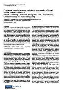
Fig. 2 The input RGB-D data to the visual odometry algorithm alongside the detected feature matches. Inliers are drawn in blue, while outliers are drawn in red.
While most visual odometry algorithms follow a common architecture, a large number of variations and specific approaches exist, each with its own attributes. The contribution of this paper is to specify the steps of our visual odometry algorithm and compare the alternatives for each step. In this section we specify these steps, and in section 4 we provide the experimental comparison of each step in the visual odometry pipeline. Our overall algorithm is most closely related to the approaches taken by Mei et al. [22] and Howard [16]. 1. Image Preprocessing: An RGB-D image is first acquired from the RGB-D camera (Fig. 2). The RGB component of the image is converted to grayscale and smoothed with a Gaussian kernel of σ = 0.85, and a Gaussian pyramid is constructed to enable more robust feature detection at different scales. Each level of the pyramid corresponds to one octave in scale space. Features at the higher scales generally correspond to larger image structures in the scene, which generally makes them more repeatable and robust to motion blur. 2. Feature Extraction: Features are extracted at each level of the Gaussian pyramid using the FAST feature detector [32]. The threshold for the FAST detector is adaptively chosen using a simple proportional controller to ensure a sufficient number of features are detected in each frame. The depth corresponding to each feature is also extracted from the depth image. Features that do not have an associated depth are discarded. To maintain a more uniform distribution of features, each pyramid level is discretized into 80×80 pixel buckets, and the 25 features in each bucket with the strongest FAST corner score are retained. 3. Initial Rotation Estimation: For small motions such as those encountered in successive image frames, the majority of a feature’s apparent motion in the image plane is caused by 3D rotation. Estimating this rotation allows us to constrain the search window when matching features between frames. We use the technique proposed by Mei et al. [22] to compute an initial rotation by directly minimizing the sum of squared pixel errors between downsampled versions of the current and previous frames. One could also use an IMU or a dynamics model of the vehicle to compute this initial motion estimate, however the increased generality of the image based rotation is preferable, while providing sufficient performance. An alternative approach would be to use a coarse-to-fine motion estimation that iteratively esti-
6
Huang et. al.
mates motion from each level of the Gaussian pyramid, as proposed by Johnson et al [17]. 4. Feature Matching: Each feature is assigned an 80-byte descriptor consisting of the brightness values of the 9 × 9 pixel patch around the feature, normalized to zero mean and omitting the bottom right pixel. The omission of one pixel results in a descriptor length more suitable for vectorized instructions. Features are then matched across frames using a mutual-consistency check. The score of two features is the sum-of-absolute differences (SAD) of their feature descriptors [16], which can be quickly computed using SIMD instructions such as Intel SSE2. A feature match is declared when two features have the lowest scoring SAD with each other, and they lie within the search window defined by the initial rotation estimation. Once an initial match is found, the feature location in the newest frame is refined to obtain a sub-pixel match. Refinement is computed by minimizing the sum-ofsquare errors of the descriptors, using ESM to solve the iterative nonlinear least squares problem [4]. We also use SIMD instructions to speed up this process. 5. Inlier Detection: Although the constraints imposed by the initial rotation estimation substantially reduce the rate of incorrect matches, an additional step is necessary to further prune away bad matches. We follow Howard’s approach of computing a graph of consistent feature matches, and then using a greedy algorithm to approximate the maximal clique in the graph [16, 14]. The graph is constructed according to the fact that rigid body motions are distance-preserving operations – the Euclidean distance between two features at one time should match their distance at another time. Thus, each feature match is a vertex in the graph, and an edge is formed between two feature matches if the 3D distance between the features does not change substantially. For a static scene, the set of inliers make up the maximal clique of consistent matches. The maxclique search is approximated by starting with an empty set of feature matches and iteratively adding the feature match with greatest degree that is consistent with all feature matches in the clique (Fig. 2). Overall, this algorithm has a runtime quadratic in the number of feature matches, but runs very quickly due to the speed of the consistency checking. In section 4, we compare this approach to RANSAC-based methods [26, 21]. 6. Motion estimation The final motion estimate is computed from the feature matches in three steps. First, an initial motion is estimated using an absolute orientation method to find the rigid body motion minimizing the Euclidean distance between the inlier feature matches [15]. Second, the motion estimate is refined by minimizing feature reprojection error. This refinement step implicitly accounts for the fact that the depth uncertainty originates from the stereo matching in image space. Finally, feature matches exceeding a fixed reprojection error threshold are discarded from the inlier set and the motion estimate is refined once again. To reduce short-scale drift, we additionally use a keyframe technique. Motion is estimated by comparing the newest frame against a reference frame. If the camera motion relative to the reference frame is successfully computed with a sufficient
Visual Odometry and Mapping for Autonomous Flight Using an RGB-D Camera
7
number of inlier features, then the reference frame is not changed. Otherwise, the newest frame replaces the reference frame after the estimation is finished. If motion estimation against the reference frame fails, then the motion estimation is tried again with the second most recent frame. This simple heuristic serves to eliminate drift in situations where the camera viewpoint does not vary significantly, a technique especially useful when hovering.
3.2 Mapping Visual odometry provides locally accurate pose estimates; however global consistency is needed for metric map generation and navigation over long time-scales. We therefore integrate our visual odometry system with our previous work in RGBDMapping [13]. This section focuses on the key decisions required for real-time operation; we refer readers to our previous publication for details on the original algorithm that emphasizes mapping accuracy [13]. Unlike the local pose estimates needed for maintaining stable flight, map updates and global pose updates are not required at a high frequency and can therefore be processed on an offboard computer. The MAV transmits RGB-D data to an offboard laptop, which detects loop closures, computes global pose corrections, and constructs a 3D log-likelihood occupancy grid map. For coarse navigation, we found a 10 cm resolution to provide a useful balance between map size and precision. Depth data is downsampled to 128×96 prior to a voxel map update to increase the update speed, resulting in spacing between rays of approximately 5 cm at a range of 6 m. Incorporating a single frame into the voxel map currently takes approximately 1.5 ms. As before, we adopt a keyframe approach to loop closure – new RGB-D frames are matched against a small set of keyframes to detect loop closures, using a fast image matching procedure [13]. New keyframes are added when the accumulated motion since the previous keyframe exceeds either 10 degrees in rotation or 25 centimeters in translation. When a new keyframe is constructed, a RANSAC procedure over FAST keypoints [32] compares the new keyframe to keyframes occurring more than 4 seconds prior. As loop closure requires matching non-sequential frames, we obtain putative keypoint matches using Calonder randomized tree descriptors [7]. We obtain a putative match for a descriptor if the L2 distance to the most similar descriptor in the other frame has a ratio less than 0.6 with the next most similar descriptor. RANSAC inlier correspondences establish a relative pose between the frames, which is accepted if there are at least 10 inliers. These inliers are determined through reprojection error, and the final refined relative pose between keyframes is obtained by solving a two-frame sparse bundle adjustment (SBA) system, which minimizes overall reprojection error. To keep the loop closure detection near constant time as the map grows, we limit the keyframes against which the new keyframe is checked. First, we only use keyframes whose pose differs from the new frame (according to the existing
8
Huang et. al.
estimates) by at most 90 degrees in rotation and 5 meters in translation. We also use Nist´er’s vocabulary tree approach [27], which uses a quantized “bag of visual words” model to rapidly determine the 15 most likely loop closure candidates. Keyframes that pass these tests are matched against new frames, and matching is terminated after the first successful loop closure. On each successful loop closure, a new constraint is added to a pose graph, which is then optimized using TORO [9]. Pose graph optimization is typically fast, converging in roughly 30 ms. Corrected pose estimates are then transmitted back to the vehicle, along with any updated voxel maps. Greater global map consistency can be achieved using a sparse bundle adjustment technique that optimizes over all matched features across all frames [20]. However, this is a much slower approach and not yet suitable for real-time operation.
3.3 State estimation and control To control the quadrotor, we integrated the new visual odometry and RGB-D Mapping algorithms into our system previously developed around 2D laser scanmatching and SLAM [3]. The motion estimates computed by the visual odometry are fused with measurements from the onboard IMU in an Extended Kalman Filter. The filter computes estimates of both the position and velocity, which are used by the PID position controller to stabilize the position of the vehicle. We keep the SLAM process separate from the real-time control loop, instead having it provide corrections for the real-time position estimates. Since these position corrections are delayed significantly from when the measurement upon which they were based was taken, we must account for this delay when we incorporate the correction by retroactively modifying the appropriate position estimate in the state history. All future state estimates are then recomputed from this corrected position, resulting in globally consistent real-time state estimates. By incorporating the SLAM corrections after the fact, we allow the real-time state estimates to be processed with low enough delay to control the MAV, while still incorporating the information from SLAM to ensure drift free position estimation.
4 Experiments This section presents results that compare our design decisions with other approaches, especially with respect to the ways these decisions affect autonomous flight. First, we compare our approach to visual odometry and mapping with alternatives. In some cases, computational speed is preferred over accuracy. Second, we present results using the RGB-D camera to stabilize and control a MAV. We characterize the performance of the system as a whole, including its limitations.
Visual Odometry and Mapping for Autonomous Flight Using an RGB-D Camera
9
Fig. 3 Panorama photograph of the motion capture room used to conduct our ground-truth experiments. Visual feature density varies substantially throughout this room.
4.1 Visual Odometry There are a variety of visual odometry methods, and the existing literature is often unclear about the advantages and limitations of each. We present results comparing a number of these approaches and analyze their performance. As is true in many domains, the tradeoffs can often be characterized as increased accuracy at the expense of additional computational requirements. In some cases, the additional cost is greatly offset by the improved accuracy. We conducted a number of experiments using a motion capture system that provides 120 Hz ground truth measurements of the MAV’s position and attitude. The motion capture environment can be characterized as a single room approximately 11m×7m×4m in size, lit by overhead fluorescent lights and with a wide variation of visual clutter – one wall is blank and featureless, and the others have a varying number of objects and visual features (see Fig. 3). While this is not a large volume, it is representative of many confined, indoor spaces, and provides the opportunity to directly compare against ground truth. We recorded a dataset of the MAV flying various patterns through the motion capture environment. Substantial movement in X, Y, Z, and yaw were all recorded, with small deviations in roll and pitch. We numerically differentiated the motion capture measurements to obtain the vehicle’s ground truth 3D velocities, and compared them to velocities and trajectories as estimated by the visual odometry and mapping algorithms. Table 1 shows the performance of our integrated approach, and its behavior when adjusting different aspects of the algorithm. Each experiment varied a single aspect from our approach. We present the mean velocity error magnitude, the overall computation time per RGB-D frame, and the gross failure rate. We define a gross failure to be any instance where the visual odometry algorithm was either unable to produce a motion estimate (e.g., due to insufficient feature matches) or where the estimated 3D velocities exceeded a fixed threshold of 1 m/s. Timing results were computed on a 2.67 GHz laptop computer. The dataset was designed to challenge vision-based approaches to the point of failure, and includes motion blur and feature-poor images, as would commonly be encountered indoors and under moderate lighting conditions. Our algorithm had a mean velocity error of 0.387 m/s and a 3.39% gross failure rate, and is unlikely to have been capable of autonomously flying the MAV through the entire recorded
10
Our approach Inlier detection RANSAC Preemptive RANSAC Greedy max-clique – our approach Initial rotation estimate None Gaussian pyramid levels 1 2 3 – our approach 4 Reprojection error minimization Bidir. Gauss-Newton Bidir. ESM – our approach Unidir. Gauss-Newton Unidir. ESM Absolute orientation only Feature window size 3 5 7 9 – our approach 11 Subpixel feature refinement No refinement Adaptive FAST threshold Fixed threshold (10) Feature grid/bucketing No grid
Huang et. al. Velocity error (m/s) 0.387 ± 0.004
% gross failures 3.39
total time (ms) 14.7
0.412 ± 0.005 0.414 ± 0.005 0.387 ± 0.004
6.05 5.91 3.39
15.3 14.9 14.7
0.388 ± 0.004
4.22
13.6
0.387 ± 0.004 0.385 ± 0.004 0.387 ± 0.004 0.387 ± 0.004
5.17 3.52 3.39 3.50
17.0 15.1 14.7 14.5
0.387 ± 0.004 0.387 ± 0.004 0.391 ± 0.004 0.391 ± 0.004 0.467 ± 0.005
3.24 3.39 3.45 3.47 10.97
14.7 14.7 14.6 14.6 14.4
0.391 ± 0.004 0.388 ± 0.004 0.388 ± 0.004 0.387 ± 0.004 0.388 ± 0.004
5.96 4.24 3.72 3.39 3.42
12.8 13.7 14.2 14.7 15.7
0.404 ± 0.004
5.13
13.1
0.385 ± 0.004
3.12
15.3
0.398 ± 0.004
4.02
24.6
Table 1 Comparison of various approaches on a challenging dataset. Error is computed using a high resolution motion capture system for ground truth.
trajectory. In contrast, in environments with richer visual features, we have observed mean velocity errors of 0.08 m/s, with no gross failures, significantly lower than the values reported in table 1. Inlier detection RANSAC based methods [26] are more commonly used than the greedy max-clique approach. We tested against two RANSAC schemes, traditional RANSAC and Preemptive RANSAC [28]. The latter attempts to speed up RANSAC by avoiding excessive scoring of wrong motion hypotheses. In our experiments, when allocated a comparable amount of computation time (by using 500 hypotheses), greedy max-clique outperformed both. Initial rotation estimation A good initial rotation estimate can help constrain the feature matching process and reduce the number of incorrect feature matches. Disabling the rotation estimate results in slightly faster runtime, but more frequent estimation failures.
Visual Odometry and Mapping for Autonomous Flight Using an RGB-D Camera
11
Gaussian pyramid levels Detecting and matching features on different levels of a Gaussian pyramid provides provides resilience against motion blur and helps track larger features. Reprojection error We compared undirectional motion refinement, which minimizes the reprojection error of newly detected features onto the reference frame, with bidirectional refinement, which additionally minimizes the reprojection error of reference features projected onto the new frame. We additionally compared a standard Gauss-Newton optimization technique with ESM. Bidirectional refinement does provide slightly more accuracy without substantially greater cost, and we found no significant difference between Gauss-Newton and ESM. Feature window size As expected, larger feature windows result in more successful motion estimation at the cost of additional computation time. Interestingly, a very small window size of 3×3 yielded reasonable performance, a behavior we attribute to the constraints provided by the initial rotation estimate. Subpixel refinement, adaptive thresholding, and feature bucketing We found the accuracy improvements afforded by subpixel feature refinement to outweigh its additional computational cost. While the lighting in the motion capture experiments did not substantially change, the adaptive thresholding still yielded a lower failure rate. We would expect the accuracy difference to be greater when flying through more varied lighting conditions. Finally, without feature bucketing, the feature detector often detects clusters of closely spaced features, which in turn confuse the matching process and result in both slower speeds and decreased accuracy. Timing On the 2.6 GHz laptop computer used for comparisons, our algorithm requires roughly 15 ms per frame. The timing per stage is as follows. Preprocessing: 2.1 ms, feature extraction: 3.1 ms, initial rotation estimation: 1.0 ms, feature matching: 6.0 ms, inlier detection: 2.2 ms, and motion estimation required less than 0.1 ms. Runtimes for the computer onboard the MAV are roughly 25 ms per frame due to the slower clock speed (1.86 GHz), but are still well within real-time.
4.2 Mapping and Autonomous Flight In addition to evaluating the visual odometry algorithms against motion capture results, we also conducted a number of autonomous flight experiments in the motion capture system and in larger environments. In these experiments, the vehicle flew autonomously with state estimates provided by the algorithms presented in this paper. The vehicle was commanded through the environment by a human operator selecting destination waypoints using a graphical interface. Figure 4 shows an example trajectory where the MAV was commanded to hover at a target point, along with statistics about how well it achieved this goal. The
12
Huang et. al. Position Hold Trajectory
Y−Deviation (m)
0.2
Metric Duration Mean speed Mean pos. deviation Max pos. deviation
0.1 0 −0.1
90 s 0.10 m/s 6.2 cm 19 cm
−0.2 −0.2
−0.1 0 0.1 X−Deviation (m)
0.2
Fig. 4 A plot showing the ground truth trajectory of the vehicle during position hold. The red dot near the center is the origin around which the vehicle was hovering. The vehicle was controlled using visual odometry, and its position measured with a motion capture system.
(a)
(b)
Fig. 5 Trajectories flown by the MAV in two navigation experiments.
ground truth trajectory and performance measures were recorded with the motion capture system. In addition to the flights performed in the small motion capture environment, we have flown in a number of locations around the MIT campus, and at the Intel Research office in Seattle. Two such experiments are shown in figure 5. As the MAV covers greater distances, the RGB-D mapping algorithm limits the global drift on its position estimates by detecting loop closures and correcting the trajectory estimates. The trajectory history can then be combined with the RGB-D sensor data to automatically generate maps that are useful both for a human operator’s situational awareness, and for autonomous path planning and decision making. While the ground truth position estimates are not available, the quality of the state estimates computed by our system is evident in the rendered point cloud. A video demonstrating autonomous flight and incremental mapping is available at: http://groups.csail.mit.edu/rrg/isrr2011-mav.
Visual Odometry and Mapping for Autonomous Flight Using an RGB-D Camera
(a)
13
(b)
Fig. 6 (a) Dense maximum-likelihood occupancy voxel map of the environment depicted in Fig. 5a, false-colored by height. Unknown/unobserved cells are also tracked, but not depicted here. (b) Using the voxel map generated for Fig. 5b, the vehicle plans a collision-free 3D trajectory (green).
4.3 Navigation Figure 6a shows an occupancy voxel map populated using the dense depth data provided by the RGB-D sensor. These occupancy maps can be used for autonomous path planning and navigation in highly cluttered environments, enabling flight through tight passageways and in close proximity to obstacles. Figure 6b shows a rendering of the MAV’s internal state estimates as it flew through the environment depicted in Figure 7b, and a path planned using the occupancy map and a simple dynamic programming search strategy. While these renderings are not necessary for obstacle avoidance, they would serve to provide a human operator with greater situational awareness of the MAV’s surrounding environment.
5 Discussion and Future Work The system described in this paper enables autonomous MAV flight in many unknown indoor environments. However, there remain a great number more challenging situations that would severely tax our system’s abilities. Motion estimation algorithms based on matching visual features, such as ours and virtually all other visual odometry techniques, do not perform as well in regions with few visual features. In large open areas, the visible structure is often far beyond the maximum range of the Kinect. As a result, the system actually performs better in cluttered environments and in close quarters than it does in wide open areas. Handling these challenges will likely require the integration of other sensors such as conventional stereo cameras or laser range-finders. As these sensors have different failure modes, they serve to complement each other’s capabilities. Additional sensing modalities can reduce, but not eliminate, state estimation failures. Further robustness can be gained by further
14
Huang et. al.
Fig. 7 Textured surfaces generated using sparse bundle adjustment, with data collected from autonomous flights.
work in designing planning and control systems able to respond appropriately when the state estimates are extremely uncertain, or to plan in ways that minimize future uncertainty [12]. Our state estimation algorithms assume a static environment, and that the vehicle moves relatively slowly. As the vehicle flies faster, the algorithms will need to handle larger amounts of motion blur, and other artifacts resulting from the rolling shutter in the Kinect cameras. Larger inter-frame motions resulting from greater speeds may in turn require more efficient search strategies to retain the real-time estimation capabilities required to control the vehicle. Relaxing the static environment assumptions will likely require better ways of detecting the set of features useful for motion estimation. When moving objects subtend a substantial portion of the visible image, the maximal clique of consistent feature matches may not correspond to the static environment. Further work is also required to improve the accuracy and efficiency of the presented algorithms. Currently, the visual odometry, sensor fusion, and control algorithms are able to run onboard the vehicle; however, even with the modifications discussed in section 3.2, the loop closing and SLAM algorithms are not quite fast enough to be run using the onboard processor. In other cases, we have actively traded estimation accuracy for computational speed. Figure 7 shows the mapping accuracy possible with further processing time, using more computationally intensive techniques presented in our previous work [13]. While the maps presented in this paper are fairly small, the methods presented scale to much larger environments. We have previously demonstrated building-scale mapping with a hand-collected data set [13], although autonomous map construction of very large spaces will require exploration algorithms that keep the vehicle well localized (e.g., in visually rich areas).
Visual Odometry and Mapping for Autonomous Flight Using an RGB-D Camera
15
6 Conclusion This paper presents an experimental analysis of our approach to enabling autonomous flight using an RGB-D sensor. Our system combines visual odometry techniques from the existing literature with our previous work on autonomous flight and mapping, and is able to conduct all sensing and computation required for local position control onboard the vehicle. Using the RGB-D sensor, our system is able to plan complex 3D paths in cluttered environments while retaining a high degree of situational awareness. We have compared a variety of different approaches to visual odometry and integrated the techniques that provide a useful balance of speed and accuracy. Acknowledgements This research was supported by the Office of Naval Research under MURI N00014-07-1-0749, Science of Autonomy program N00014-09-1-0641 and the Army Research Office under the MAST CTA. D.M. acknowledges travel support from P. Universidad Cat´olica’s School of Engineering. P.H. and D.F. are supported by ONR MURI grant number N00014-09-11052, and by the NSF under contract number IIS-0812671, as well as collaborative participation in the Robotics Consortium sponsored by the U.S Army Research Laboratory under Agreement W911NF-10-2-0016.
References 1. M. Achtelik, A. Bachrach, R. He, S. Prentice, and N. Roy. Stereo vision and laser odometry for autonomous helicopters in gps-denied indoor environments. In Proceedings of the SPIE Unmanned Systems Technology XI, volume 7332, Orlando, F, 2009. 2. S. Ahrens, D. Levine, G. Andrews, and J.P. How. Vision-based guidance and control of a hovering vehicle in unknown, GPS-denied environments. In IEEE Int. Conf. Robotics and Automation, pages 2643–2648, May 2009. 3. A. Bachrach, R. He, and N. Roy. Autonomous flight in unknown indoor environments. International Journal of Micro Air Vehicles, 1(4):217–228, December 2009. 4. S. Benhimane and E. Malis. Improving vision-based control using efficient second-order minimization techniques. In IEEE Int. Conf. Robotics and Automation, Apr. 2004. 5. Michael Bl¨osch, Stephan Weiss, Davide Scaramuzza, and Roland Siegwart. Vision based mav navigation in unknown and unstructured environments. In IEEE Int. Conf. Robotics and Automation, pages 21–28, 2010. 6. G. Buskey, J. Roberts, P. Corke, and G. Wyeth. Helicopter automation a using a low-cost sensing system. Computing Control Engineering Journal, 15(2):8 – 9, april-may 2004. 7. M. Calonder, V. Lepetit, and P. Fua. Keypoint signatures for fast learning and recognition. In European Conference on Computer Vision, pages 58–71, 2008. 8. K. Celik, Soon J. Chung, and A. Somani. Mono-vision corner SLAM for indoor navigation. In IEEE International Conference on Electro/Information Technology, pages 343–348, 2008. 9. G. Grisetti, S. Grzonka, C. Stachniss, P. Pfaff, and W. Burgard. Estimation of accurate maximum likelihood maps in 3D. In IEEE Int. Conf. on Intelligent Robots and Systems, 2007. 10. G. Grisetti, C. Stachniss, S. Grzonka, and W. Burgard. A tree parameterization for efficiently computing maximum likelihood maps using gradient descent. In Proceedings of Robotics: Science and Systems, 2007. 11. C. Harris and M. Stephens. A combined corner and edge detector. In Alvey vision conference, pages 147–151, 1988.
16
Huang et. al.
12. R. He, S. Prentice, and N. Roy. Planning in information space for a quadrotor helicopter in a gps-denied environments. In IEEE Int. Conf. Robotics and Automation, pages 1814–1820, Los Angeles, CA, 2008. 13. Peter Henry, Michael Krainin, Evan Herbst, Xiaofeng Ren, and Dieter Fox. RGB-D Mapping: Using depth cameras for dense 3d modeling of indoor environments. In Int. Symposium on Experimental Robotics, Dec. 2010. 14. H. Hirschmuller, P.R. Innocent, and J.M. Garibaldi. Fast, unconstrained camera motion estimation from stereo without tracking and robust statistics. In Proc. Int. Conference on Control, Automation, Robotics and Vision, volume 2, pages 1099 – 1104, dec. 2002. 15. B. K. P. Horn. Closed-form solution of absolute orientation using unit quaternions. J. Optical Society of America, 4(4):629–642, 1987. 16. A. Howard. Real-time stereo visual odometry for autonomous ground vehicles. In IEEE Int. Conf. on Intelligent Robots and Systems, Sep. 2008. 17. A. E. Johnson, S. B. Goldberg, Y. Cheng, and L. H. Matthies. Robust and efficient stereo feature tracking for visual odometry. In IEEE Int. Conf. Robotics and Automation, Pasadena, CA, May 2008. 18. M. Kaess, A. Ranganathan, and F. Dellaert. iSAM: Incremental smoothing and mapping. IEEE Trans. on Robotics (TRO), 24(6):1365–1378, Dec 2008. 19. Jonathan Kelly and Gaurav S. Sukhatme. An experimental study of aerial stereo visual odometry. In Proc. Symp. Intelligent Autonomous Vehicles, Toulouse, France, Sep 2007. 20. K. Konolige. Sparse Sparse Bundle Adjustment. In Proc. of the British Machine Vision Conference (BMVC), 2010. 21. K. Konolige, M. Agrawal, and J. Sola. Large-scale visual odometry for rough terrain. In Int. Symp. Robotics Research, Hiroshima, Japan, 2007. 22. C. Mei, G. Sibley, M. Cummins, P. Newman, and I. Reid. A constant time efficient stereo slam system. In British Machine Vision Conference, 2009. 23. L. Meier, P. Tanskanen, F. Fraundorfer, and M. Pollefeys. Pixhawk: A system for autonomous flight using onboard computer vision. In IEEE Int. Conf. Robotics and Automation, May 2011. 24. H. Moravec. Obstacle avoidance and navigation in the real world by a seeing robot rover. PhD thesis, Stanford University, 1980. 25. P. Newman, G. Sibley, M. Smith, M. Cummins, A. Harrison, C. Mei, I. Posner, R. Shade, D. Schr¨oter, L. Murphy, W. Churchill, D. Cole, and I. Reid. Navigating, recognising and describing urban spaces with vision and laser. Int. Journal of Robotics Research, 28(11-12), 2009. 26. D. Nist´er, O. Naroditsky, and J. Bergen. Visual odometry. In Computer Vision and Pattern Recognition, pages 652–659, Washington, D.C., Jun. 2004. 27. D. Nist´er and H. Stewenius. Scalable Recognition with a Vocabulary Tree. In Computer Vision and Pattern Recognition, 2006. 28. David Nist´er. Preemptive RANSAC for live structure and motion estimation. Machine Vision and Applications, 16:321–329, 2005. 29. E. Olson, J. Leonard, and S. Teller. Fast iterative optimization of pose graphs with poor initial estimates. In IEEE Int. Conf. Robotics and Automation, pages 2262–2269, 2006. 30. M. Pollefeys, D. Nister, J.-M. Frahm, A. Akbarzadeh, P. Mordohai, B. Clipp, C. Engels, D. Gallup, S.-J. Kim, P. Merrell, C. Salmi, S. Sinha, B. Talton, L. Wang, Q. Yang, H. Stewenius, R. Yang, G. Welch, and H. Towles. Detailed Real-Time Urban 3D Reconstruction From Video. Int. J. Computer Vision, 72(2):143–67, 2008. 31. PrimeSense. http://www.primesense.com. 32. E. Rosten and T. Drummond. Machine learning for high-speed corner detection. In European Conference on Computer Vision, 2006. 33. N. Snavely, S. Seitz, and R. Szeliski. Photo tourism: Exploring photo collections in 3D. In ACM Transactions on Graphics (Proc. of SIGGRAPH), 2006. 34. B. Triggs, P. McLauchlan, R. Hartley, and A. Fitzgibbon. Bundle adjustmenta modern synthesis. Vision algorithms: theory and practice, pages 153–177, 2000.