Visual Recognition in Art using Machine Learning - University of Oxford

Visual Recognition in Art using Machine Learning

Elliot Joseph Crowley Jesus College University of Oxford Supervised by Professor Andrew Zisserman Submitted: Trinity Term 2016 This thesis is submitted to the Department of Engineering Science, University of Oxford, in fulfilment of the requirements for the degree of Doctor of Philosophy

Abstract This thesis is concerned with the problem of visual recognition in art – such as finding the objects (e.g. cars, cows and cathedrals) present in a painting, or identifying the subject of an oil portrait. Solving this problem is extremely beneficial to art historians, who are often interested in determining when an object first appeared in a painting or how the portrayal of an object has evolved over time. It allows them to avoid the unenviable task of finding paintings for study manually. However, visual recognition of art is a challenging problem, in part due to the lack of annotation in art. A solution is to train recognition models on natural, photographic images. These models have to overcome a domain shift when applied to art. Firstly, a thorough evaluation of the domain shift problem is conducted for the task of image classification in paintings; the performance of natural image-trained and paintingtrained classifiers on a fixed set of paintings are compared for both shallow (Fisher Vectors) and deep image representations (Convolutional Neural Networks – CNNs) to examine the performance gap across domains. Then, we show that this performance gap can be ameliorated by classifying regions using detectors. We next consider the problem of annotating gods and animals on classical Greek vases, starting from a large dataset of images of vases with associated brief text descriptions. To solve this, we develop a weakly supervised learning approach to solve the correspondence problem between the descriptions and unknown image regions. Then, we study the problem of matching photos of a person to paintings of that person, in order to retrieve similar paintings given a query photo. We show that performance at this task can be improved substantially by learning with a combination of photos and paintings – either by learning a linear projection matrix common across facial identities, or by fine-tuning a CNN. Finally, we present several applications of this research. These include a system that learns object classifiers on-the-fly from images crawled off the web, and uses these to find a variety of objects in very large datasets of art. We show that this research has resulted in the discovery of over 250,000 new object annotations across 93,000 paintings on the public Art UK website.

ii

Acknowledgements I would like to thank Andrew Zisserman for being such an excellent supervisor. I am grateful to my friends at Jesus College and my labmates for making my time at Oxford enjoyable. I would like to thank my parents, Julie and Joseph, and the rest of my family for their love and support. Finally, a big thank you to my wife, Hannah, for being awesome.

Contents

1 Introduction

1

1.1

Objective and Motivation . . . . . . . . . . . . . . . . . . . . . . . . . .

1

1.2 1.3

Challenges . . . . . . . . . . . . . . . . . . . . . . . . . . . . . . . . . . . Contributions and thesis outline . . . . . . . . . . . . . . . . . . . . . . .

3 4

1.4

Publications . . . . . . . . . . . . . . . . . . . . . . . . . . . . . . . . . .

6

2 Background

8

2.1

Art Studies . . . . . . . . . . . . . . . . . . . . . . . . . . . . . . . . . .

8

2.2

Computer Vision Techniques . . . . . . . . . . . . . . . . . . . . . . . . . 2.2.1 Shallow Methods for Image Classification . . . . . . . . . . . . . .

12 12

2.2.2

Deep Methods for Image Classification . . . . . . . . . . . . . . .

14

Domain Adaptation Techniques . . . . . . . . . . . . . . . . . . . . . . .

16

2.3.1

Adaptating to Art . . . . . . . . . . . . . . . . . . . . . . . . . .

19

3 Image Classification in Paintings 3.1 Datasets . . . . . . . . . . . . . . . . . . . . . . . . . . . . . . . . . . . .

21 21

2.3

3.2 3.3

3.4

3.1.1

The Paintings Dataset . . . . . . . . . . . . . . . . . . . . . . . .

22

3.1.2

VOC12 . . . . . . . . . . . . . . . . . . . . . . . . . . . . . . . . .

22

3.1.3 Google Images . . . . . . . . . . . . . . . . . . . . . . . . . . . . . Classifying Paintings using Shallow Representations . . . . . . . . . . . .

26 26

3.2.1

Results . . . . . . . . . . . . . . . . . . . . . . . . . . . . . . . . .

27

Classifying Paintings using Deep Representations . . . . . . . . . . . . .

30

3.3.1 3.3.2

Networks . . . . . . . . . . . . . . . . . . . . . . . . . . . . . . . Augmentation . . . . . . . . . . . . . . . . . . . . . . . . . . . . .

30 31

3.3.3

Implementation details . . . . . . . . . . . . . . . . . . . . . . . .

33

Summary . . . . . . . . . . . . . . . . . . . . . . . . . . . . . . . . . . .

34

iv

4 Detecting Object Regions in Paintings 4.1 Re-ranking Paintings using Discriminative Regions

. . . . . . . . . . . .

35 35

4.1.1

Spatial consistency using discriminative patches . . . . . . . . . .

36

4.1.2

Experiments . . . . . . . . . . . . . . . . . . . . . . . . . . . . . .

39

4.2

Classification by Detection using a Region-CNN . . . . . . . . . . . . . . 4.2.1 Combining deep detection and classification . . . . . . . . . . . .

47 50

4.3

Summary . . . . . . . . . . . . . . . . . . . . . . . . . . . . . . . . . . .

52

5 Object Detection in Classical Art

53

5.1

Data – the Beazley Vase Archive . . . . . . . . . . . . . . . . . . . . . .

55

5.2 5.3

Text mining for visually consistent clusters . . . . . . . . . . . . . . . . . Searching for Candidate Regions . . . . . . . . . . . . . . . . . . . . . . .

56 59

5.4

Training Strong Detectors . . . . . . . . . . . . . . . . . . . . . . . . . .

62

5.5

Results . . . . . . . . . . . . . . . . . . . . . . . . . . . . . . . . . . . . .

63

5.6

Summary . . . . . . . . . . . . . . . . . . . . . . . . . . . . . . . . . . .

70

6 Face Recognition in Art 6.1 Motivation and Approach . . . . . . . . . . . . . . . . . . . . . . . . . .

71 71

6.2

Learning to improve photo-painting based retrieval of faces . . . . . . . .

76

6.2.1

L2 Distance . . . . . . . . . . . . . . . . . . . . . . . . . . . . . .

76

6.2.2 6.2.3

Discriminative Dimensionality Reduction (DDR) . . . . . . . . . . Learning Classifiers . . . . . . . . . . . . . . . . . . . . . . . . . .

76 77

6.2.4

Network Fine-tuning . . . . . . . . . . . . . . . . . . . . . . . . .

78

Data for retrieving faces in paintings . . . . . . . . . . . . . . . . . . . .

78

6.3.1 6.3.2

Image Sources . . . . . . . . . . . . . . . . . . . . . . . . . . . . . Datasets . . . . . . . . . . . . . . . . . . . . . . . . . . . . . . . .

78 79

6.4

Implementation details for face retrieval . . . . . . . . . . . . . . . . . .

83

6.5

Face retrieval experiments . . . . . . . . . . . . . . . . . . . . . . . . . .

84

6.6 6.7

Retrieving Photos of Faces using Paintings . . . . . . . . . . . . . . . . . Summary . . . . . . . . . . . . . . . . . . . . . . . . . . . . . . . . . . .

88 89

6.3

7 Applications and Demos 7.1

7.2 7.3

90

Class-based Retrieval of Paintings . . . . . . . . . . . . . . . . . . . . . .

91

7.1.1

Retrieving Colours in Paintings . . . . . . . . . . . . . . . . . . .

96

7.1.2 Retrieving Textures in Paintings . . . . . . . . . . . . . . . . . . . More efficient collection of annotation by Crowdsourcing . . . . . . . . .

96 99

7.2.1

Annotation Procedure and Results . . . . . . . . . . . . . . . . .

99

Longitudinal Studies using Retrieved Paintings . . . . . . . . . . . . . . .

103

v

7.4

Finding Objects in Paintings on-the-fly . . . . . . . . . . . . . . . . . . . 7.4.1 Evaluation of the on-the-fly system . . . . . . . . . . . . . . . . .

106 107

7.4.2

Searching the British Library . . . . . . . . . . . . . . . . . . . .

110

7.5

Detecting Objects in Paintings on-the-fly . . . . . . . . . . . . . . . . . .

112

7.6

7.5.1 Evaluation of the detection system . . . . . . . . . . . . . . . . . Finding Doppelgangers in Art . . . . . . . . . . . . . . . . . . . . . . . .

114 116

7.7

Summary . . . . . . . . . . . . . . . . . . . . . . . . . . . . . . . . . . .

119

8 Conclusion 8.1

120

Achievements . . . . . . . . . . . . . . . . . . . . . . . . . . . . . . . . .

120

8.2 Suggestions for Future Research . . . . . . . . . . . . . . . . . . . . . . . Bibliography . . . . . . . . . . . . . . . . . . . . . . . . . . . . . . . . . . . .

122 124

vi

Chapter 1:

1.1

Introduction

Objective and Motivation

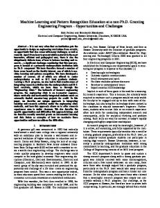
The ambiguous face of the Mona Lisa. The wild brushstrokes of Van Gogh. The melted clocks of Dali. Depictions of tales on Ancient Greek vases. Art has a way to entrance us and provoke thought – particularly modern art, which in the past tended to provoke feelings of bewilderment and confusion. It also raises questions. Consider figure 1.1. In the painting (a), is that a dog running along the leaves? How might we find similar such paintings? Upon witnessing the painting (b), a train enthusiast might wonder how the depiction of steam trains has varied across time. On the detail of a classical vase given in (c), who exactly is that seated figure? The painting (d) is entitled Portrait of an Unknown Woman. Can we find out who she is? The objective of this thesis is recognising the visual content of such art using machine learning. Through this, these questions can be answered. As well as sating our collective curiosity, this recognition is extremely beneficial to art historians, who are often interested in determining when an object (e.g. a dog, a skull, a car) first appeared in a painting or how the portrayal of an object has evolved over time. To achieve this they have the unenviable task of finding paintings for study manually, an extremely arduous and time-consuming process. However, if a machine could recognise the objects in a painting then works containing a particular object could be retrieved instantly, without any human effort. This would allow art historians to spend less time searching for art and more time studying it. Fortunately, visual object recognition is a field that has seen tremendous advances

2

1.1. Objective and Motivation

(a)

(b)

(c)

(d)

Figure 1.1: A selection of art, used to motivate the research conducted in this thesis. (a), (b), and (d) are oil paintings from the Art UK dataset [1]. (c) is a detail of a Greek vase from the Beazley Archive [2].

in recent years, notably due to the widespread induction of deep Convolutional Neural Networks (CNNs). However, the vast majority of research conducted is concerned with recognition in the domain of natural images (i.e. everyday photos taken with a camera). Common benchmarks to evaluate recognition performance are large, annotated datasets of natural images (e.g. PASCAL VOC [46] and ILSVRC [106]). There is very little research on examining recognition in the domain of art. Rectifying this is another of our driving motivations.

1.2. Challenges

1.2

3

Challenges

Annotation in Art. Natural images annotated with objects are everywhere – large numbers of annotated photos are readily available in curated datasets [42, 46] and simply typing the name of an object into Google Image search [8] will produce high quality images of that object. This allows for the learning of powerful visual models that recognise a wide-range of object categories. AlexNet [78] for instance was trained on the trainval (Training + Validation) set of ILSVRC-2012 – a subset of ImageNet [42] – which consists of 1.2 million natural images each annotated with one of a thousand categories. Such widespread annotation does not exist for paintings. This presents two challenges: the first is how to cope with limited annotation and the second, is how to obtain more annotation in an automated, efficient manner. Domain Shift. Due to the lack of annotated art, it is often necessary to learn models from natural images and apply these to paintings. This introduces a domain shift problem as natural images and paintings can have very different low-level statistics. A learnt model should ideally be able to adapt to the new domain, however several studies [26, 118] have shown that there is typically a significant drop in performance when models are learnt in one domain and applied to another. Variation in Art. Paintings can vary considerably in depiction style from photorealistic renderings through particular movements (e.g. Impressionism, Pointillism) to more abstract depictions (Fauvism, Cubism). Such stylistic variations can be seen for a highland cow in figure 1.2. There are also temporal differences in the depiction of objects in paintings. For example, dogs appear in paintings not only as beloved pets, but also in hunting scenes where they are often significantly smaller. Most photos of cars contain modern cars, whereas some paintings of cars will be vintage; photographs of planes will typically be of modern commercial jetliners whereas those in paintings can be more akin to Wright Flyers or Spitfires.

1.3. Contributions and thesis outline

4

Figure 1.2: Various stylistic interpretations of a highland cow. Notice that some paintings are quite photo-realistic while others lean towards abstraction.

1.3

Contributions and thesis outline

Image Classification in Paintings. Chapter 3. Here, we examine the domain shift problem of applying natural image-trained classifiers to paintings, by comparing their performance to painting-trained classifiers (which do not experience any domain shift) at the same task. We introduce datasets from which to learn and apply classifiers, and evaluate both shallow and deep feature representations. We show that there is a performance gap between natural image-trained and painting-trained classifiers, and that for deep architectures this gap reduces as the classifiers get better (i.e. classification performance correlates with increased domain invariance). We also show that deep classifiers substantially outperform their shallow counterparts. Detecting Object Regions in Paintings. Chapter 4. In this chapter, we explore the benefits of classifying regions within images rather than the whole image as in Chapter 3

1.3. Contributions and thesis outline

5

by using detectors. We show that for natural image-trained classifiers learnt on shallow features it is possible to reduce the aforementioned performance gap by re-ranking paintings with high classification scores based on their spatial consistency with natural images containing the same object. We also show that the gap can be reduced using a deep detection network, which is able to outperform higher-complexity classification networks. This network is able to locate very small objects that are otherwise missed out. Object Detection in Classical Art. Chapter 5. This chapter presents a weakly supervised learning method for annotating gods (and animals) in a dataset of Greek vases of antiquity. This method utilises the short text descriptions supplied with each vase to isolate vases containing a god in a consistent pose. A form of multiple-instance learning is then used to locate regions likely to contain the god, and these are used to train a Deformable Part [50] model which is applied to the remainder of the dataset. Face Recognition in Art. Chapter 6. Inspired by the tale of a man who found himself in a painting (figure 6.1), we study whether it is possible to retrieve paintings of people given their photo. We show that it is indeed possible, and compare shallow and deep feature representations for the task. We further demonstrate that performance can be improved further through additional learning, including (i) learning a linear projection to apply to the features using discriminative dimensionality reduction, and (ii) refining the features produced by a deep network, by fine-tuning it with both photos and paintings. As a coda, we demonstrate that the reverse of this task is also achievable by using paintings to retrieve photos of faces from a large corpus. Applications and Demos. Chapter 7. This chapter describes the applications and demos borne from the research conducted in this thesis. First, we show that classifiers learnt from a pool of 10,000 tagged paintings (by tagged, we mean annotated by the public) are able to retrieve paintings from among 200,000 unannotated works with high precision, thereby providing thousands of potential new tags for free. These retrieved

1.4. Publications

6

paintings are then used in conjunction with a web server, allowing members of the public to efficiently and quickly confirm which of these new tags are correct. Next, we introduce an on-the-fly system that allows a user to search through hundreds of thousands of paintings, for objects of their choosing in real-time: the user provides a query which is used to crawl the web for images. These images are used to learn a classifier that is applied to a corpus of paintings, which are then ranked and retrieved by classifier score. We further improve on this by providing a detection system which returns the exact regions in paintings containing objects. This has the added advantage of being able to locate very small objects. Finally, we build a demo based on the research of Chapter 6 where a user may submit a photo of their face, and very similar faces in paintings will be retrieved. 1.4

Publications

The research conducted in this thesis has resulted in five peer-reviewed publications listed below in chronological order: • E. J. Crowley and A. Zisserman. Of Gods and Goats: Weakly supervised learning of figurative art. In Proc. BMVC, 2013. [36] • E. J. Crowley and A. Zisserman. The State of the Art: Object retrieval in paintings using discriminative regions. In Proc. BMVC, 2014. [38] • E. J. Crowley and A. Zisserman. In Search of Art. In Workshop on Computer Vision for Art Analysis, ECCV, 2014. [37] • E. J. Crowley, O. M. Parkhi, and A. Zisserman. Face Painting: querying art with photos. In Proc. BMVC, 2015. [35] • E. J. Crowley and A. Zisserman. The Art of Detection. In Workshop on Computer Vision for Art Analysis, ECCV, 2016. [39] The domain shift work of Chapter 3 and the detection work of Chapter 4 are presented in [38, 39]. The research for object detection in antiquity appeared in [36]. Our work on

1.4. Publications

7

face retrieval in paintings is presented in [35]. Finally, our on-the-fly system of Chapter 7 first featured in [37].

Chapter 2:

Background

In this chapter, we review a range of literature that serves as suitable background for the research conducted in this thesis. Firstly in section 2.1 to motivate the task of visual recognition in art, we explore a variety of art history studies, each of which could benefit from computer vision techniques. Secondly, in section 2.2 we provide a review of feature representations for images which are essential for visual recognition, and how they have advanced throughout the years, from hand-crafted features based on gradients to representations obtained from deep, non-linear neural networks. Finally, in section 2.3 we review literature for techniques on domain adaptation. This is of particular relevance to us, as in this thesis we are often concerned with the task of learning in the domain of natural images, and adapting this to the domain of paintings. 2.1

Art Studies

For as long as there has been art, there have been those who have studied it. Art history is the study of art and how it varies (e.g. in style or genre) across time. This extends to the depiction of specific objects or entities in art, so image classification and retrieval systems are of immense benefit to the field. In this section, we give examples of literature in the field that could indeed benefit from the application of computer vision. Several studies are concerned with the depiction of a particular object. One study [73] examines depictions of skulls in paintings and how they convey the theme of memento mori (or, “Remember that you must die”), due to their placement next to objects such as flickering candles, or wilting flowers (figure 2.1, left). Further to this, they propose

2.1. Art Studies

9

that drawings of skulls produced by the anatomist Andreas Vesalius in his book – On the Fabric of the Human Body – deploy visual strategies to counter this theme, as it was making the study of the human body difficult. Such visual strategies include placing skeletons in casual poses with whimsical facial expressions (figure 2.1, right).

Figure 2.1: Two works containing skulls that convey different themes. Left: Aelbert van der Schoor, Still Life with Skulls, c. 1650. Oil on canvas. Right: Andreas Vesalius, Skeleton Contemplating a Skull, 1543. Woodcut from page 164 of On the Fabric of the Human Body.

Another study [117] explores the depiction of dogs in the work of Rembrandt. In these works the dog tends to be doing its own thing such as scratching its ear, paying no attention to its surroundings, even as some dramatic event occurs nearby (such as in figure 2.2). They conclude from such depictions that dogs mirror unenlightened humans. More modern art is also subject to analysis: the work of [33] explores the depictions of cars in 1960s art. For example, consider figure 2.3: the advertisement (a) places a car next to a glamorous woman in an attempt to make it appear desirable. (b) links the car to the negative aspects of industrial capitalism; there is a solidier, a fat cat, and plenty of pollution present in the painting. (c) shows the car next to human bodies, emphasising their danger. Unsurprisingly, humans are a popular subject for study. The work of Burke [24] questions the modern understanding of the Italian Renaissance nude. They observe woodcuts depicting travellers encountering naked natives (see figure 2.4) and conclude that this is a possible influence to Renaissance depictions of nudity.

2.1. Art Studies

10

Figure 2.2: Rembrandt van Rijn, The Presentation in the Temple, c. 1637-41. Notice that the dog (lower-left corner) has its back turned to what is going on and is scratching its ear. The work of [117] concludes that the dog represents an unenlightened person.

Figure 2.3: (a) Advert for B. H. Wragges in Harper’s Bazaar, no. 3012, November 1962, page 22. (b) Andre Fougeron, Atlantic Civilization, 1953. (c) A detail of Andy Warhol, Green Car Crash, 1963.

2.1. Art Studies

11

Figure 2.4: Left: Unknown Illustrator, Columbus’ First Voyage to the New World, 1493. Right: Unknown Illustrator, Amerigo Vespucci’s Voyage to the New World, 1505.

Another work [76] observes a piece by Signorelli (figure 2.5(a)), showing a man in a state of undress with grey arms, a drooping face and folded ears. From these features they believe that the man is close to death, and search for other portraits displaying such signs. These include (b) and (c) in figure 2.5 which both contain men with drooping expressions and dead eyes.

Figure 2.5: (a) Luca Signorelli, Virgin and Child with Saint John the Baptist and a Donor, c. 1491-94. (b) Austrian artist, Portrait of Rudolf IV of Austria, c. 1365. (c) Monogrammist AA, The Corpse of Maximilian I, 1519

Such works could all benefit from the application of computer vision methods. For example, for [73] a classifier could be used to isolate additional paintings containing skulls.

2.2. Computer Vision Techniques

12

A detector would be able to speed up searching for the small dogs presented in [117]. 2.2

Computer Vision Techniques

Image Classification is the task of classifying an image by the object/s it contains. This is a challenging task as the assorted objects in an image can be at a variety of scales, may be occluded or truncated. Several objects can assume one of many different poses. Furthermore, lighting in images is prone to extreme variety. An image in terms of its pixels is a poor way of describing its object content (for example, the pixels of a cow in a dark room, and a cow outdoors in sunshine will bear no resemblance). Because of this an image is usually represented by a feature: a vector describing the discriminative elements within an image, which is ideally invariant to scale, pose, occlusion et cetera. Such features may be used to learn classifiers which can then be applied to other features. Several challenging datasets of natural, photographic images such as PASCAL VOC [46], the SUN Attribute dataset [100], and ILSVRC [106] provide a means to evaluate the performance of such features. In this section, we examine hand-crafted, or shallow feature representations (section 2.2.1) which were prevalent for many years, as well as more recent deep representations (section 2.2.2) which now dominate the field. 2.2.1

Shallow Methods for Image Classification

Computing a (shallow) feature vector for an image typically consists of two steps: (i) Many local descriptors are extracted from the image – this can be either done densely (sampled at regular intervals in the image) or sparsely (sampled at specific saliencies in the image). (ii) These descriptors are then combined or encoded in some manner to form a feature vector of fixed dimensionality. These feature vectors can then be used to learn classifiers e.g. with positive and negative samples of a particular class in a Linear-SVM. Note that there are alternatives to following these steps. The GIST feature [92] directly produces a global representation of an image by splitting it into a grid, computing


13

an orientation histogram for each grid entry, and concatenating them. The local descriptors used are largely based around recording gradient information, and include SIFT [86] and SURF [21]. In [15] the authors observe that simply squarerooting SIFT descriptors before they are encoded sees a boost in the power of the resultant feature vectors for a variety of tasks. The remainder of this section is concerned with the various encoding methods used on these descriptors. For a more comprehensive review on descriptor encoding, see the excellent work of Chatfield et al. [28]. Many descriptor encoding methods are a variant of the ‘Bag of Visual Words’ approach of Sivic and Zisserman [115] which describes a given image as a histogram of visual words. Firstly, a vocabulary of D ‘words’ is learnt by performing K-means clustering on a wealth of SIFT descriptors. The centre of each K-means cluster is considered to be a ‘word’. To produce a feature vector for an image, its SIFT descriptors are extracted; each SIFT descriptor is assigned to a word, corresponding to the nearest cluster centre. The resulting feature vector is a D-dimensional histogram of these words. The work of [82] improves on this method by introducing some geometry to the feature vector. They represent the image as a ‘Spatial Pyramid’ – at level 1 of the pyramid a 1 ⇥ 1 grid splits the image into 1, at level 2, a 2 ⇥ 2 grid splits the image into 4 etc. This effectively describes the image as a series of crops at different scales and positions. A feature vector is computed for each crop as in [115] and these are concatenated. A disadvantage of the ‘Bag of Visual Words’ approach is that when a local descriptor is quantised to a fixed word, information is lost. This is ameliorated by Jégou [69] who use a VLAD feature representation: instead of recording the number of extracted descriptors assigned to each word, they instead record the mean of the assigned descriptors relative to each word. Unfortunately, the resulting feature vector is now d times larger than for bag of words, where d is the dimensionality of the local descriptors. The popular Improved Fisher Vector [101] representation is again a variant of [115]. Instead of learning a vocabulary of words with K-means, a Gaussian Mixture model is


14

used. This allows a descriptor to be assigned to multiple centres with different weights. The mean descriptor relative to each word is calculated as well as the covariance, retaining even more information than VLAD. Fisher Vectors have not only been shown to perform very well on standard image classification tasks but also for the specialist task of face classification; in [112] the authors show that a Fisher Vector face representation performs well on the LFW benchmark [66]. They further improve this by discriminatively reducing the dimension of the Fisher Vector by optimising a classification loss for positive and negative image pairs, an idea first explored for faces in [59]. 2.2.2

Deep Methods for Image Classification

Deep learning in the context of this thesis refers to the utilisation of Convolutional Neural Networks (CNNs). These networks consist of a series of sequential layers (the depth of the network is the number of these layers), each of which contains numerous filters (or neurons) which are convolved with a given input to produce an output. For illustration, let us consider a layer to which the input is a square image with width and height L. The image has T colour channels, so let’s treat the image as having a thickness of T , It can therefore be represented by a L ⇥ L ⇥ T cube. The layer consists of N filters, each of which is an l ⇥ l ⇥ T cube. When the input is convolved with a filter, with stride n, the response is X ⇥ X ⇥ 1 where X is ⇠ L/n. The responses of all these filters are concatenated to produce a X ⇥ X ⇥ N output. A non-linear operation is applied to the output of a layer before it is input to a new layer. This allows the network to describe complex non-linear transformations. In the past CNNs saw some use, such as for the task of character recognition [83, 84] but were not widespread until fairly recently as they were hampered by two severe limitations: (i) the need for very large amounts of data, and (ii) the requirement for substantial computational power. The seminal work of Krizhevsky et al. [78] is arguably the first showcase of the power of the CNN in vision. Their network architecture – reproduced in figure 2.6 – consists of five convolutional layers, followed by three fully


15

Figure 2.6: The AlexNet Architecture, reproduced from [78]. This network consists of 5 convolutional layers and 3 fully connected layers. Note that the network filters are split into two streams because of memory constraints on the GPU. This is no longer necessary with modern GPUs.

connected layers1 . The non-linear operation used between layers is the rectifier – f (x) = max(0, x) – which is frequently referred to as ReLU. They train the network using the trainval set of ILSVRC-2012 [106] which consists of over 1 million images, each with a single label corresponding to one of 1,000 object classes. The output of the network is a 1000-D soft-max vector corresponding to the probability of an image belonging to each class. The network is trained on a GPU, batches of images are put through the network and their soft-max vectors are used in conjunction with the correct labels in a logistic loss. The gradient of this loss is back-propagated through the network, updating its filters – this is stochastic gradient descent (SGD). The resulting network obtained an excellent top-5 error rate of 15.3% on the test set of ILSVRC-2012, compared to 26.2% using a shallow Fisher Vector representation. Since AlexNet, more powerful network architectures have emerged. Chatfield et al. [29] learn 8-layer networks as in [78], but add more filters to the layers as well as lower strides – their CNN-M and CNN-S networks have stride 2 in the first convolutional layer instead of AlexNet’s stride 4, and 512 filters in the third and fourth layer. CNN-M and CNNS obtain top-5 error rates of 13.7% and 13.1% on ILSVRC-2012 respectively. Simonyan and Zisserman [113] show that performance can be improved even further using very deep 1A

fully connected layer is simply a convolutional layer where each filter is the same size as the input.

2.3. Domain Adaptation Techniques

16

network architectures (16-19 convolutional layers) with very small 3 ⇥ 3 filters in each layer. A fusion of such architectures gives a top-5 error rate of 6.8%. Residual Networks, developed by He et al. [64] represent groups of convolutional layers as residual blocks, this allows for extremely deep architectures (they evaluate these networks for up to 152 layers). A fusion of these networks gives a top-5 error rate of 3.57% on the test set of ILSVRC-2012. CNNs not only exhibit excellent performance on the task they were trained for but also, at adapting to other tasks. Girshick et al. [57] fine-tune a variation of AlexNet [78] for PASCAL VOC classification, that had already been learnt for ImageNet classification as above. They do this by replacing the final 1 ⇥ 1 ⇥ 1000 layer (which outputs a 1000-D vector) with a 1⇥1⇥21 layer – the output of which is 21-D, one for each class in PASCAL VOC and another for ‘background’. They then perform SGD for windows from PASCAL VOC to update the network. Several works [44, 93, 102] have demonstrated that the intermediate representations produced by the CNNs – such as the 4096-D vector output of the penultimate convolutional layer of AlexNet – can be used as all-purpose features for images, and may be used to learn classifiers that excel at a variety of tasks. 2.3

Domain Adaptation Techniques

Domain Adaptation is a frequently occurring scenario in machine learning. It occurs when a model is learnt from data drawn from a source domain, and is applied to a data drawn from a differing target domain. A good probabilistic introduction to this phenomenon is given in [116] and there are extensive literature reviews on the topic [71, 99]. It is not a problem to be taken lightly as several studies [26, 118] have shown that there is a significant drop in performance when classifiers are learnt from one domain and applied to another. Here, we discuss a selection of interesting papers on the topic for shallow and deep representations. These typically address one of two scenarios: 1. There are class labels for data in both the source and target domain (for the same

17


set of classes). 2. There are only class labels for data in the source domain. The target domain data is unlabelled. Then, in section 2.3.1 we address papers that deal with the adaptation most relevant to this thesis: the case where one domain is art. Shallow Domain Adaptation. There is a wealth of literature on adapting handcrafted (i.e. shallow) features between domains. [41] takes the very simple approach of augmenting the feature space of both the source and target data; assuming each datum (both source and target) is a N dimensional vector x, the source data is instead represented as

s,

and the target data as

t

s

where:

= [x, x, 0]

t

= [x, 0, x]

(2.1)

and 0 is a N dimensional zero vector. These representations are then used as input to standard machine learning algorithms (e.g. SVMs). Others [67, 94] have instead reweighted source samples based on target sample similarity. Saenko et al. [107] consider the case where one has access to a large amount of data from a source domain, and very little from a target domain – this is an example of the first scenario mentioned at the beginning of this section. They aim to learn a non-linear transformation that compensates for differences in the two domains. This is achieved by considering similar examples (i.e. those with the same class label) across domains in some feature space and learning the transformation such that they are moved closer together. Kulis et al. [79] build on this by learning asymmetric transformations that can move examples in a target domain directly to the source domain (and vice versa). This has the added advantage of allowing source and target data to be described in different features spaces with different dimensionalities. Sub-space based methods for adaptation are prevalent: Gopalan et al. [58] acknowl-


18

edge that it is not always possible to have labelled data in the target domain (the second scenario mentioned at the start of this section), and propose an unsupervised method for generating an intermediate subspace between that of the source and target domain. They do this by the viewing the feature spaces of the source and target domains as points on a Grassmann manifold, and sample points along the geodesic between them. Fernando et al. [52] build on this by representing each domain as an eigenvector, and optimise a matrix transformation between domains. Interestingly, the optimal mapping turns out to be the covariance matrix between the source and target eigenvectors. The vast majority of these approaches assume a fixed target distribution; Hoffman et al. [65] instead consider cases where the target distribution evolves over time (e.g. the feed from a traffic camera, at different times of day and for different weather conditions). They develop an adaptation scheme which models these changing distributions by forming incremental, sample-dependent adaptive kernels. Deep Domain Adaptation. More recent works have been focused on incorporating adaptation into deep neural architectures, allowing for end-to-end learning. Ganin and Lempitsky [54] start with an AlexNet architecture [78] pre-trained on ImageNet and add a new branch to the network at the output of the fourth convolutional layer. This branch consists of two fully connected layers and a classification layer, as with the original branch. The classifier is two-way however, and classifies an input sample as being from one of two domains. When losses are back-propagated from this branch to the original network, the gradient is reversed. The idea being that this should create a domain-invariant network. This is an example of Scenario 2, as the target data is not used with any class labels. Tzeng et al. [119] improve this on architecture idea. They start with a pre-trained Caffenet [70] (which has the same structure as an AlexNet) and supplement the classification loss with two additional losses: a ‘domain confusion’ loss and a ‘domain classifier’ loss. The output of ‘fc7’ is applied to a new fully connected layer ‘fcD’ and the two dimensional output of this is used for these losses. The domain classifier loss is similar to


19

that used in [54] and classifies samples into the correct domain. The opposing ‘domain confusion’ loss forces samples from different domains to appear similar to the network. These two opposing losses are are optimised iteratively, and constantly test the ability of the network to produce domain-invariant features. Also of note is the interesting work of Aljundi and Tuytelaars [14]. They propose a method that uses a small number of samples from a target domain to modify filters in the first convolutional layer of a network that are badly affected by domain shift. The modifications are based on filters that are less affected by the domain shift. 2.3.1

Adaptating to Art

In the vast majority of the domain adaptation literature, the source and target domains comprise natural images drawn from two different distributions; frequently evaluation is carried out on the ‘Office Dataset’ [107] where the domains in questions are images taken with a DSLR camera, a webcam, and images from the Amazon website. Here we specifically discuss work where one of the domains comprises art. Shrivastava et al. [111] consider cross-domain matching (e.g. from a painting of the Arc De Triomphe to a photo). They utilise an Exemplar-SVM [87] to discover what is unique or ‘salient’ about an image with respect to its dataset of origin and use this information for matching. This does not require a domain-specific representation. Aubry et al. [17] take the interesting approach of matching 3D renderings of buildings such as Notre Dame Cathedral to paintings. They first render 2D views of the building and then find mid-level discriminative patches [18, 74, 114] (MLDPs), and filter patches that are unstable when the view-point changes. They then match these patches to similar patches on paintings. These patches demonstrate remarkable invariance between paintings and renderings. Wu and Hall [122, 123] study the problem of generalising across depiction styles. They build a multi-layer depiction-invariant graph model, and show that it is capable of generalising to drawings and cartoons in particular. However, a limitation of their method is that it is restricted in both training and testing to uncluttered Caltech101 [48]


20

style images – where the object of interest fills the image against a uniform background. Natural image-trained detectors have seen some success when applied to art: Ginosar et al. [55] apply different face detectors to the abstract Cubist paintings of Picasso. Surprisingly, they find that DPMs outperformed R-CNNs [124] at this task, and conclude that R-CNNs overfit to natural images and fail at adapting to paintings. However, it could be that R-CNNs are not strictly part-based, and the DPMs excel at finding realistic looking face-parts within the paintings. Cai et al. [26] demonstrate that DPMs learnt on natural images are able to find objects in art, and utilise query expansion to refine the model with confident artwork detections. Redmon et al. [103] provide a deep object detection system learnt on natural images, and apply it to the Picasso dataset of [55] and the People-Art dataset of [25]. The performance is very successful; they surmise that although at a pixel level, art and natural images differ, it’s the similarity in size and shape of the objects that is important.

Chapter 3:

Image Classification in Paintings

In this chapter, we consider the task of image classification – classifying an image by the objects it contains – in paintings by learning image-level classifiers (i.e. representing an entire image by a single vector). We are particularly interested in the domain shift problem of learning such classifiers from natural images and applying them to paintings, and to what extent this can be rectified with a good feature representation. This shift can be evaluated by comparing classifiers trained on natural images to those trained on paintings. To this end, we introduce datasets of natural images and paintings from which to learn and evaluate classifiers (section 3.1). We compare classifiers learnt with shallow features in 3.2, and deep features in section 3.3. 3.1

Datasets

In this section we describe the datasets used in this chapter: one of the datasets – the Paintings Dataset (section 3.1.1) consists entirely of paintings and is split into a training, validation and test set. The training and validation (trainval) sets are used to learn image-level classifiers in the painting domain – these are essentially the gold standard to which natural image-trained classifiers are compared. The test set is used to evaluate all classifiers (both natural image-trained and painting-trained). Two datasets of natural images are used purely to train classifiers – both consist of only training and validation sets. One is a subset of the PASCAL VOC 2012 [46] dataset (section 3.1.2) and the other is crawled from Google Images (section 3.1.3).

3.1. Datasets

3.1.1

22

The Paintings Dataset

We construct the Paintings Dataset which is used to assess classification performance throughout this chapter. It is a subset of the publicly available Art UK dataset [1] (formerly known as ‘Your Paintings’) consisting of over 210,000 oil paintings. 10,000 of these have been annotated as part of the ‘Tagger’ project whereby members of the public tag the paintings with the objects that they contain. The subset is obtained by searching Art UK for annotations and painting titles corresponding to the classes of the PASCAL VOC dataset [46]. With tags and titles complete annotation is assumed in the VOC sense – that each painting has been annotated for all VOC categories – as long as ‘people’ are ignored, as this particular class has a tendency of appearing frequently without being acknowledged. Thus, the ‘person’ class is not considered, and also we do not include classes that lack a sufficient number of tags (cat, bicycle, bus, car, motorbike, bottle, potted plant, sofa, tv/monitor). Paintings are included for the remaining classes – aeroplane, bird, boat, chair, cow, dining table, dog, horse, sheep, train. These are split at random into training, validation and test sets. The statistics for this dataset are given in table 3.1, and example class images are shown in figures 3.1 and 3.2. The URLs for the paintings in this dataset are provided at the website [12]. 3.1.2

VOC12

The dataset we use primarily to train natural-image classifiers is the VOC12 dataset. This is the subset of PASCAL VOC 2012 [46] trainval images that contain any of the 10 classes of the Paintings Dataset. Note that although detailed region-level annotation is provided, these are not used in this chapter – classifiers are learnt using whole images. Example images in this dataset are given in figure 3.3. The statistics for this dataset are also given in table 3.1.

23

3.1. Datasets

Aeroplane

Bird

Boat

Chair

Cow

Figure 3.1: Example class images from the Paintings Dataset. From top to bottom row: aeroplane, bird, boat, chair, cow. Notice that the dataset is challenging: objects have a variety of sizes, poses and depictive styles, and can be partially occluded or truncated.

24

3.1. Datasets

Dining table

Dog

Horse

Sheep

Train

Figure 3.2: Further example class images from the Paintings Dataset. From top to bottom row: dining table, dog, horse, sheep, train.

25

3.1. Datasets

Dataset

Split Aero Bird Boat Chair Cow Din Dog Horse Sheep Train Total

Paintings Train Dataset

VOC12

Val

74 319 862

493 255 485 483

656

270

13

140

52 130 113

127

76

569 318 586 549

72 222

130 3463 35

865

Test

113 414 1059

710

405

164 4301

Total

200 805 2143 1202 625 1201 1145 1493

751

329 8629

Train

327 395 260

566 151 269 632

237

171

273 3050

Val

343 370 248

553 152 269 654

245

154

271 3028

Total

670 765 508 1119 303 538 1286

482

325

544 6078

Google

Train

90

90

90

90

90

90

90

90

90

90

900

Images

Val

10

10

10

10

10

10

10

10

10

10

100

100 100 100 100

100

100

Total

100 100 100

100 1000

Table 3.1: The statistics for the datasets used in this chapter: each number corresponds to how many images contain that particular class. Note, because each image can contain multiple classes, the total across the row does not equal the total number of images. Train/Validation/Test splits are also given.

Figure 3.3: Example images from VOC12. Note that images often contain multiple classes and the objects exist at a wide variety of scales and poses, and are frequently occluded or truncated. Top row (l-r): Examples from the ‘aeroplane’, ‘bird’ and ‘boat’ class. Middle row (l-r): ‘chair’, ‘cow’, ‘dining table’. Bottom row (l-r): ‘dog’, ‘horse’, ‘sheep’, ‘train’.

3.2. Classifying Paintings using Shallow Representations

3.1.3

26

Google Images

Another dataset used for training natural-image classifiers is the Google Images dataset. This consists of images mined from Google Image Search for the categories used in VOC12, manually filtered to remove erroneous examples. The statistics for this dataset are given in table 3.1 and example images are given in figure 3.4.

Figure 3.4: Example images from the Google Images dataset. Notice that the object in each case tends to occupy a large part of the image and is fairly central. Top row (l-r): Examples from the ‘aeroplane’, ‘bird’, ‘boat’ and ‘chair’ class. Middle row (l-r): ‘cow’, ‘dining table’, ‘dog’. Bottom row (l-r): ‘horse’, ‘sheep’, ‘train’.

3.2

Classifying Paintings using Shallow Representations

In this section, we compare image-level classifiers trained on shallow features from natural images (the trainval set of VOC12 or the trainval set of Google Images) to classifiers trained on shallow features from paintings (the trainval set of the Paintings Dataset). In both cases these classifiers are evaluated on the test set of the Paintings Dataset. The classifiers trained on paintings are representative of the ‘best-case scenario’ since there is no domain shift to the target domain. Performance is assessed using Average


27

Precision (AP) per class, and also Precision at rank k (Prec@k) – the fraction of the top-k retrieved paintings that contain the object – as this places an emphasis on the accuracy of the highest classification scores when k is low. The classifiers used are linear one-vs-rest SVMs, and the features are produced using Fisher Vectors. Fisher Vector Representation. Fisher vectors are generated for each image using the pipeline of [28], with the implementation available from the website [5]: RootSIFT [15] features are extracted at multiple scales from each image. These are reduced using PCA to 80-D and augmented with (x,y) coordinates. The features are encoded with a 512 component Gaussian Mixture Model to form a 83,968D Fisher Vector [101] feature for each image. Implementation. Linear-SVM Classifiers are learnt using the training features per class in a one-vs-the-rest manner for assorted weightings of the regularisation term (the weight parameter is denoted as C). The C that produces the highest AP for each class when the corresponding classifier is applied to the validation set is recorded. The training and validation features are then combined to train classifiers using these C parameters. These classifiers are then applied to the test features, which are ranked by classifier score. Finally, these ranked lists are used to compute AP and Prec@k. 3.2.1

Results

The per class AP results are given in table 3.2 along with their mean (mAP). Prec@k results are given in table 3.3 and the mean plots of these are shown in figure 3.5. It can be seen that for all classes there is a drop in performance when training on natural images compared to training on paintings. The drop depends on the class, for example it is small for ‘boat’ and large for ‘cow’. It is surprising that the performance drop is not higher for vehicle classes considering that these have evolved significantly from their earlier forms in paintings to those in modern natural images. The explanation is probably that there are still key discriminative elements present in both cases, for example most images and

28


Training Data

Aero Bird Boat Chair Cow Dtable Dog Horse Sheep Train mAP

Paintings Dataset 0.61 0.36

0.89

0.67 0.43

0.62 0.39

0.68

0.58

0.77

0.60

VOC12

0.32 0.17

0.71

0.35 0.21

0.33 0.22

0.44

0.24

0.63

0.36

Google Images

0.24 0.14

0.60

0.11 0.12

0.25 0.18

0.42

0.23

0.44

0.27

Table 3.2: Average Precision for Classification Performance on the test set of the Paintings Dataset where Fisher Vector classifiers are learnt from the training set of (i) Paintings Dataset, (ii) VOC12, (iii) Google Images. Notice the large gap in performance between painting trained classifiers and natural image trained classifiers

paintings of boats will still contain masts and water irrespective of the time period. Overall, there is a drop in mPrec@k from 0.98 (paintings) to 0.66 (VOC images) at k = 5, and from 0.91 to 0.63 at k = 20, i.e. a significant difference. A similar drop in mPrec@k also occurs for classifiers trained on Google Images. This performance drop is also reflected in the mean Average Precision (mAP) where the mAP drops from 0.59 for classifiers trained on paintings to 0.36 for classifiers trained on VOC images. Later in the thesis, in section 4.1, we demonstrate that this performance drop can be reduced by re-ranking paintings based on their spatial consistency with natural images of an object category.

29


TrainSet

k Aero Bird Boat Chair Cow Dtab Dog Horse Sheep Train Mean

Art UK

5

1.00 1.00

1.00

1.00 1.00

1.00 0.80

1.00

1.00

1.00

0.98

VOC12

5

0.80 0.40

1.00

0.60 0.00

1.00 0.40

1.00

0.60

0.80

0.66

Google Images

5

1.00 0.20

0.40

0.20 0.20

0.60 0.80

1.00

0.60

1.00

0.60

Art UK

10

1.00 1.00

1.00

1.00 0.80

0.90 0.80

1.00

1.00

1.00

0.95

VOC12

10

0.80 0.40

1.00

0.50 0.10

0.90 0.40

0.90

0.50

0.90

0.64

Google Images 10

0.90 0.10

0.70

0.10 0.30

0.50 0.50

0.90

0.70

0.80

0.55

Art UK

20

0.95 0.90

1.00

0.95 0.75

0.90 0.70

0.95

1.00

1.00

0.91

VOC12

20

0.65 0.35

0.95

0.55 0.20

0.70 0.60

0.85

0.50

0.95

0.63

Google Images 20

0.65 0.20

0.80

0.10 0.30

0.40 0.35

0.85

0.60

0.85

0.51

Table 3.3: Prec@k on the test set of the Paintings Dataset using Fisher Vector classifiers learnt from different training sets. Notice the large gap in performance between the classifiers trained on paintings and those trained on natural images.

Figure 3.5: Mean Prec@k on the test set of the Paintings Dataset using Fisher Vector classifiers learnt from different training sets.

3.3. Classifying Paintings using Deep Representations

3.3

30

Classifying Paintings using Deep Representations

In this section, we again compare image-level classifiers trained on features from natural images (VOC12) to classifiers trained on features from paintings (the training set of the Paintings Dataset) as in section 3.2. However, the features considered here are produced by an assortment of different neural network architectures. In section 3.3.1 we determine how the mAP gap – the change in mean (over class) AP between natural image and painting-trained classifiers – is affected by the CNN architecture used to produce the feature, and in section 3.3.2 we discuss train and test augmentations, and the per class performance. Implementation details are given in section 3.3.3. 3.3.1

Networks

Three networks are compared, each trained on the ILSVRC-2012 [106] image dataset with batch normalisation [68]: first, the VGG-M architecture of Chatfield et al. [29] that consists of 8 convolutional layers. The filters used are quite large (7 ⇥ 7 in the first layer, 5 ⇥ 5 in the second). The features produced are 4096-D. Second, the popular ‘very deep’ model of Simonyan and Zisserman [113] VD-16 that consists of 16 convolutional layers with very small 3 ⇥ 3 filters in each layer of stride 1. The features produced are again 4096-D. Third, the ResNets of He et al. [64] that treat groups of layers in a network as residual blocks relative to their input. This allows for extremely deep network architectures. The 152-layer ResNet model RES-152 is selected for this work. The features extracted are 2048-D. Network comparison. Table 3.4 gives the mAP performance for the three networks trained on VOC12 or the Paintings Dataset. Four things are clear: firstly, and unsurprisingly when we compare this to table 3.2 it is clear that deep features outperform shallow ones; second, for features from the same network, classifiers learnt on paintings are better at retrieving paintings than classifiers learnt on natural images; third, RES-

31


Net

Training Set

none

f5

f25 Stretch mAP gap

VGG-M VOC12

50.8 51.9 52.9

52.9

VGG-M Paintings Dataset

65.1 67.8 67.8

67.8

VD-16

VOC12

54.8 56.2 56.7

56.8

VD-16

Paintings Dataset

68.7 71.2 71.2

70.8

RES-152 VOC12

60.5 61.6 62.0

62.3

RES-152 Paintings Dataset

72.5 74.6 74.6

75.0

14.9

14.0

12.7

Table 3.4: mAP for CNN-based image-level classifiers trained on VOC12 vs the Paintings Dataset. Both the networks used to generate the features and the augmentation schemes are varied. ‘Net’ refers to the network used. ‘none’, ‘f5’, ‘f25’ and ‘Stretch’ are augmentation schemes and each column gives the corresponding mAP. Augmentation schemes are described further in section 3.3.2. The last column shows the gap in mAP between natural image and painting-trained classifiers for ‘Stretch’ augmentation.

152 features surpass VD-16 features, which in turn surpass VGG-M features; and finally, that the mAP gap decreases as the network gets better – from a 14.9% difference for VGG-M to a 12.7% for RES-152. Thus, improved classification performance correlates with increased domain invariance. Note that for some classes there are an unbalanced number of trainval samples. However, there does not seem to be an obvious correlation with performance; aeroplane classifiers learnt on paintings significantly outperform those learnt on photos despite being trained with far fewer positive samples (87 vs. 670). 3.3.2

Augmentation

Four augmentation schemes available in the MatConvNet toolbox [120] are compared, and are applied to each image to produce N crops. In all cases the image is first resized (with aspect ratio preserved) such that its smallest length is 256 pixels. Crops extracted are ultimately 224 ⇥ 224 pixels. The schemes are: none, a single crop (N=1) is taken from the centre of the image; f5, crops are taken from the centre and the four corners. The same is done for the left-right flip of the image (N=10); f25, an extension of f5.

32


Crops are taken at 25% intervals in both width and height, this is also carried out for the left-right flip (N=50); and finally, Stretch, a random rectangular region is taken from the image, linear interpolation across the pixels of the rectangle is performed to turn it into a 224 ⇥ 224 crop, there is then a 50% chance that this square is left-right flipped. This is performed 50 times (N=50). Note that the same augmentation scheme is applied to both training and test images. Set

Metric

VOC AP Prec@k=20

Aero

Bird Boat Chair Cow Dtab

Dog Horse Sheep Train Avg.

69.4

42.0

50.5

88.7

100.0 100.0 100.0

57.3 62.4

48.4

73.5

48.7

81.9 62.3

85.0 90.0 100.0 100.0 100.0 100.0 100.0 97.5

Prec@k=50

94.0

94.0 100.0

72.0 84.0

92.0 100.0 100.0

98.0 100.0 93.4

Prec@k=100

61.0

82.0

99.0

72.0 89.0

84.0

98.0 100.0

86.0

98.0 86.9

77.1

54.1

94.3

78.7 68.3

76.3

62.7

68.8

85.7 75.0

Paint AP

83.5

Prec@k=20

95.0 100.0 100.0 100.0 95.0

95.0 100.0 100.0 100.0 100.0 98.5

Prec@k=50

96.0 100.0 100.0

98.0 92.0

94.0 100.0 100.0 100.0 100.0 98.0

Prec@k=100

65.0 100.0

97.0 90.0

92.0

99.0

98.0 100.0

91.0 100.0 93.2

Table 3.5: Retrieval performance comparison on the test set of the Paintings Dataset for classifiers trained using ResNet features. The images have been augmented using ‘Stretch’. ‘Set’ refers to the training set used and the performance metric is given under ‘Metric’: Average Precision (AP) or Precision at rank k (Prec@k).

Results and discussion. Table 3.4 shows that the type of augmentation is important: ‘stretch’ generally produces the highest performance – a 2% or more increase in mAP over ‘none’, and equal to or superior to ‘f5’ and ‘f25’. This is probably because the stretch augmentation also mimics foreshortening caused by out-of-plane rotation for objects. Table 3.5 shows the per class AP and Prec@k for the best performing case (ResNet with stretch augmentation), with the corresponding PR curves given in figure 3.6. Natural image-trained classifiers are clearly inferior to painting-trained classifiers, with an AP gap of around 0.1 for most classes. Prec@k sees a similar decrease. There are some particularly bad cases: ‘sheep’ has a colossal 20% decrease in AP, ‘dog’ experiences a large 12% drop.


33

Figure 3.6: Precision-Recall curves for different classes, comparing natural image-trained (red) and painting-trained (blue) classifiers learnt on ResNet features. Notice for ‘sheep’ that the gap in the curves is very noticeable even at low recall.

There are several reasons for this: a few of the paintings are depicted in a highly abstract manner, understandably hindering classification. Furthermore, some objects are depicted in a particular way in paintings that isn’t present in natural images, e.g. aeroplanes in paintings can be WWII spitfires rather than commercial jets. However, in spite of many paintings being depicted in quite a natural way, there is a problem with small objects. Some examples of paintings containing small objects that have been ‘missed’ (i.e. received a low classifier score) are given in figure 3.7. We investigate this problem later in the thesis, in section 4.2. 3.3.3

Implementation details

Each image in both the training and test set first undergoes augmentation to produce N crops. The mean RGB values of ILSVRC-2012 are subtracted from the respective colour channels of each crop. These crops are then passed into a given network, and the outputs of the layer before the prediction layer are recorded, giving N feature vectors. These are

3.4. Summary

34

Figure 3.7: Examples of paintings where a small object has been ‘missed’ (i.e. given a low score) by a classifier. In each case, the object under consideration is indicated by a red box. Top row (l-r): aeroplane, dog. Bottom row (l-r): sheep, chair.

averaged and then L2 normalised to produce a single feature. Linear-SVM Classifiers are then learnt as in section 3.2. 3.4

Summary

In this chapter we have examined the domain shift problem of classifying paintings using classifiers learnt from natural images by comparing these to classifiers learnt from paintings, for both shallow and deep features. Unsurprisingly, the performance of deep representations surpasses that of their shallow counterparts. We have also observed that classification performance correlates with increased domain invariance for deep architectures. Later, in Chapter 6 we show that we are able to reduce the domain shift for the task of face retrieval, through joint training with both natural images and paintings.

Chapter 4:

Detecting Object Regions in Paintings

In the previous chapter, we performed image classification on paintings by considering whole images. In this chapter we perform image classification by instead considering regions within images. The idea being that only the most salient regions, directly pertaining to object classes are considered rather than background clutter. This chapter is divided into two parts. The first part (section 4.1) is concerned with improving ‘shallow’ classification performance using handcrafted mid-level patches. The second (section 4.2) improves ‘deep’ performance using a neural network which utilises image regions. In more detail, in section 4.1 we show that we are able to reduce the performance gap between natural image-trained classifiers and painting-trained classifiers for a Fisher Vector image representation (section 3.2) by re-ranking the paintings with the highest classifier scores based on their spatial consistency with natural images of an object category. This method utilises mid-level discriminative patches (MLDPs). In section 4.2 we perform classification-by-detection (i.e. finding regions in an image and classifying them) using the Faster R-CNN network [104] and demonstrate that this gives better performance than classifying whole images using a more complicated ResNet architecture. 4.1

Re-ranking Paintings using Discriminative Regions

In section 3.2 we showed, somewhat surprisingly, that image classifiers learnt from VOC12 images (section 3.1.2) with a Fisher Vector representation can classify paintings containing an object class with some success. In this section, we introduce a method of re-ranking

4.1. Re-ranking Paintings using Discriminative Regions

36

these classifier results by considering the spatial consistency of MLDP correspondences, and show that the precision of the top-classified paintings in the test set of the Paintings Dataset can be significantly improved based on how spatially consistent the paintings are with the natural images used to train the classifiers. More formally, we are concerned with improving Precision at k (the fraction of the top-k retrieved paintings that contain the class) for low values of k. The baseline results for the Fisher Vector classifiers are given in table 3.3 and the class mean, mPrec@k in figure 3.5. We also compare other methods of training and re-ranking including training from Google Images – where the images are more Caltech101 [48] style – and using a DPM [50] detector, and also investigate hybrid re-ranking strategies. 4.1.1

Spatial consistency using discriminative patches

Here, we describe our method for establishing and measuring spatial consistency between objects in the training images and objects in the paintings. The consistency scores obtained by this method will be used in section 4.1.2 for re-ranking the top ranked (i.e. high classification score) paintings in the test set of the Paintings Dataset for each class. The method proceeds in three stages: (i) a set of MLDPs are generated for each trainval image in the VOC12 dataset for a class (e.g. for trains); (ii) classifiers are learnt from these patches and applied as sliding window detectors to find the highest scoring regions in the paintings, leading to a set of putative correspondences; lastly, (iii), a RANSAC [53]-style algorithm is used to select a subset of these correspondences that are spatially consistent, and each painting is scored based on the size of this subset. We use MLDPs here for two reasons: first, because they can be obtained with minimal supervision; and second, since an MLDP covers only part of an object (rather than all of it), they are more tolerant to viewpoint and intra-class variation. (i) Obtaining discriminative patches. Aubry et al. [17] provide a fast method for choosing a set of MLDPs and ranking the discriminability of these regions in an image: if q is a descriptor of an image region, µ the mean of those descriptors in a dataset, and ⌃


37

the covariance then the discriminability | (q)| can be measured as in (4.1). This describes how the patch differs from the mean of the dataset in a whitened space.

| (q)|2 = (q

µ)T ⌃ 1 (q

µ)

(4.1)

Here we use the HOG descriptor [40], and obtain the D most discriminative patches for each training image. This forms the set of MLDPs for each image. Some examples of high scoring regions for VOC12 are shown in figure 4.1.

Figure 4.1: A subset of discriminative regions (blue) overlapping with VOC12 ROIs (red). Notice that informative areas of the objects are picked out such as a horse’s head, and even within the ROI no indiscriminate background patches are selected.

Implementation details. Each VOC12 training image is annotated with a Region of Interest (ROI) for each object instance in that image. Candidate square-shaped regions that overlap with the ROI are extracted from each image (and its left-right flipped version) at 3 scales per octave. For each of these a contrast-sensitive 5 ⇥ 5 HOG descriptor with 8 ⇥ 8 pixel cells is formed using the implementation of [50] resulting in a 775-D vector. µ and ⌃ are obtained from the training set using the method of [62] with a window size of 20 pixels. Squares are ranked and selected according to | (q)|. Low gradient regions are ignored. Non-maximal suppression is performed using an intersection over union of 0.5 between squares as a threshold and the top D squares are retained. (ii) Putative correspondences using MLDPs. The correspondences between the set of MLDPs in an image and a painting are established by using the patch as a detector. A Linear Discriminate Analysis (LDA) classifier [62], w, is learnt for each MLDP (i.e. the discriminative squares) in the natural image as in (4.2). LDA allows for efficient


38

training of detectors without the need to mine for hard negatives, greatly cutting down the time required for training.

w = ⌃ 1 (q

µ)

(4.2)

Each MLDP is used as a sliding-window detector in the manner of [50], and the highest scoring detection window on the painting is recorded. This gives a provisional correspondence (x1 , y1 , x2 , y2 , s) where (x1 , y1 ) is the centre of the discriminative region used to train the classifier, (x2 , y2 ) is the centre of the highest scoring detection window and s is the scale change between the two windows. The set of MLDPs creates a set of provisional correspondences between the regions used to train the classifiers in the natural image and the regions corresponding to the highest scoring detections in the painting. (iii) Enforcing spatial consistency between correspondences. Given the set of provisional correspondences between a training set image and a painting, we now obtain a subset of these that are spatially consistent. This is achieved by fitting a linear spatial mapping. Correspondences that do not agree with this mapping are considered erroneous and removed, this enforces spatial consistency between correspondences. The mapping is a restricted similarity homography [63] that allows the object in the natural image to be uniformly scaled and translated to the painting but not rotated as: 2 3 2 32 3 2 3 6 x2 7 6 s 0 7 6 x1 7 6 t x 7 4 5=4 54 5 + 4 5 y2 0 s y1 ty

(4.3)

The best mapping is obtained using a RANSAC-style approach: for an image-painting pair each provisional correspondence (x1 , y1 , x2 , y2 , s) can be used to form an estimation of the mapping (4.3). The number of other correspondences within a scale and distance threshold of this mapping are considered to be inliers and tallied. Each correspondence is evaluated exhaustively and the mapping that produces the highest number of inliers is assumed to be the best mapping. These inliers are then used to compute an affine


39

homography, which allows for rotation and shearing, and the number of inliers is reestimated to provide a score. In the following subsection this score will be used to re-rank images. Results. Figure 4.2 shows example image-painting pairs before and after enforcing spatial consistency. It can be seen that the combination of discriminative patches (that are able to ignore ‘background’ regions) together with the spatial consistency is able to overcome the problem of background clutter – i.e. other objects in the paintings. The method is able to match class instances despite significant scale changes, and also to match parts of objects when there is partial occlusion. 4.1.2

Experiments

In this subsection we demonstrate that rankings on the test set of Paintings Dataset obtained with the VOC12 Fisher Vector classifiers of section 3.2 can be improved by (i) re-ranking the high-scoring paintings using spatially consistent sets of MLDPs. We also compare (ii) using a DPM for re-ranking, and (iii) training on the Google Images set (described in section 3.1.3) instead of on VOC12 images. Finally (iv) we consider hybrid re-ranking strategies. (i) Discriminative patch re-ranking using VOC12 images.

We start from the

Paintings Dataset test set rankings obtained by the classifiers trained on the VOC12 trainval images, and investigate how the re-ranking performance is affected by the number of MLDPs, D, used for each training image; and by the number, N , of paintings that are re-ranked (i.e. only the top N classifier ranked paintings are considered). We observe the effect of varying the parameters N , D on mPrec@k for low k’s to determine what provides the best performance. The effect of varying N on mPrec@k for low k is shown in figure 4.3(a) for fixed D = 100. Initially, precision increases with N , but as N gets too large (for example exceeds the number of positives ranked well by the classifier) the performance declines,


40

Figure 4.2: Image-painting pair correspondences before (left) and after (right) computing a spatially consistent subset. Note, that the MLDP correspondences are able to generalise slightly over viewpoint, intra-class differences, and between natural images and paintings.


41

as the scoring provided by the classifier rankings are then of no benefit (if N is equal to the number of paintings, then this disregards the initial ranking). In general, mPrec@k increases with D as there needs to be sufficient patches to cover all the salient areas of the object in the image – though eventually there is insufficient increase to warrant the extra computation. In the following we set N = 60 & D = 100 to achieve high Prec@k for low k’s. Results. Prec@k curves for selected classes before and after re-ranking are given in the first row of figure 4.4. Prec@k for all classes is shown in table 4.1 and mean Prec@k plots are given in figure 4.5. Notice that the performance at low k’s is improved by MLDP reranking for almost every class; this is because for most classes an object in a painting will strongly resemble the same object in one of the natural images for that class, differing only by scale and translation with minimal rotation, allowing consistent regions to be located using MLDPs. Consider a cow; it is usually an unrotated rectangular entity, rarely seen from above – there is little variety in its pose so it is very likely that for a painting of a cow there will be a similar natural image. This also applies to isolated parts of more deformable objects; although the body of a dog is highly deformable, its face is not and will be consistent between some natural image-painting pairs. The top ranked paintings after re-ranking for selected classes are displayed in figures 4.6 and 4.7. The one class that does not improve is dining table. This class is highly prone to variety, a dining table can be seen from many angles, is often covered with other objects, and often heavily occluded. There is very little consistency between natural imagepainting pairs. (ii) DPM re-ranking using VOC12. Here, we return to the rankings obtained with the baseline classifiers of section 3.2, and re-rank using a Deformable Part Model (DPM) [50] object category detector, instead of a set of MLDPs. DPMs excel at finding spatially consistent object regions, and thus provide a natural comparison to the MLDP method.


(a)

42

(b)

Figure 4.3: mPrec@k as (a) N varies, and (b) as ↵ varies, where ↵ controls the MLDP vs DPM score weighting of the hybrid re-ranking scheme.

Figure 4.4: Prec@k on the test set of the Paintings Dataset for training on VOC12 images (top row), Google Images (middle row); and VOC12 images (bottom row) with hybrid re-ranking. The green curves show the perfect re-ranking of the top N classified paintings for each class.

For each class, a DPM is learnt using class ROIs as positive examples and other regions as negative examples as in [50]. Each DPM has 6 components and 8 parts. These are then applied to the top N ranked test set paintings of the Paintings Dataset in a sliding window cascade [49] and the score corresponding to the highest detection is recorded. The paintings are then re-ranked by this score. N = 60 is used to allow for direct comparison with MLDP re-ranking.

43


Ranking

k Aero Bird Boat Chair Cow Dtab Dog Horse Sheep Train Mean

MLDP

5 1.00 0.60 1.00

0.60 0.60 0.40 1.00

1.00

1.00 1.00

0.82

Classifier 5 0.80 0.40 1.00

0.60 0.00 1.00 0.40

1.00

0.60 0.80

0.66

MLDP

10 0.80 0.40 1.00

0.70 0.40 0.50 0.80

1.00

0.80 1.00

0.74

Classifier 10 0.80 0.40 1.00

0.50 0.10 0.90 0.40

0.90

0.50 0.90

0.64

MLDP

15 0.67 0.47 1.00

0.60 0.33 0.53 0.73

1.00

0.67 1.00

0.70

Classifier 15 0.73 0.47 0.93

0.60 0.20 0.80 0.53

0.87

0.47 0.93

0.65

MLDP

20 0.75 0.50 1.00

0.55 0.35 0.65 0.65

1.00

0.65 0.95

0.71

Classifier 20 0.65 0.35 0.95

0.55 0.20 0.70 0.60

0.85

0.50 0.95

0.63

Table 4.1: Prec@k on the test set of the Paintings Dataset before and after MLDP re-ranking using VOC12 training images. MLDP improves Prec@k in almost all instances.

Figure 4.5: Mean Prec@k on the test set of the Paintings Dataset before and after MLDP re-ranking using VOC12 training images. Hybrid scoring schemes are also shown, which improve precision even further.

Results. The Prec@k curves for DPM re-ranking for selected classes are also given in the first row of figure 4.4. DPM re-ranking performs better than MLDP re-ranking for


44

Figure 4.6: Top 10 ranked paintings after re-ranking using MLDP for aeroplanes and chairs. A green border indicates a correct classification and a red border an incorrect one.


45

Figure 4.7: Top 10 ranked paintings after re-ranking using MLDP for dogs and sheep. A green border indicates a correct classification and a red border an incorrect one.


46

objects that appear in the most generic poses; for example, a cow is usually either at front or side profile. For such classes object instances will strongly resemble one of the DPMs components – generalised from many training examples. However, for objects that assume many different poses like dog, MLDP re-ranking proves more successful as each dog only has to have a part (e.g. face) in common with a natural image rather than an entire pose in common with many. (iii) Re-ranking using Google Images. Here, learning classifiers and re-ranking are performed using the Google Images set (described in section 3.1.3). Note that these classifiers were learnt in section 3.2. There are three key differences between this and VOC12; (i) the images are less cluttered with more centred objects like those in Caltech101, (ii) there are far fewer images, (iii) no ROI is provided, so the entire image is used as the ROI. MLDP re-ranking and DPM re-ranking are performed in the same manner as in (i) and (ii) where both MLDP extraction and DPM training are performed on Google Images. DPMs have been trained previously using the entire image as the ROI, but for scene classification [95]. The Prec@k curves for selected classes for both MLDP and DPM re-ranking are given in the second row of figure 4.4. MLDP re-ranking generally outperforms DPM re-ranking. This is because with a small training set it is difficult for a DPM to generalise the poses of an object, whereas for MLDP it is simply required that there exists an image resembling the pose of a painting. Note that MLDPs are able to localise an object even without the correct ROI being provided. (iv) Hybrid re-ranking strategies. MLDPs and DPMs succeed in different scenarios; a DPM will often find the entirety of an object, whereas MLDP will find salient parts, (face, legs). A combination of these two measures can provide a good understanding of what an object is. A simple linear weighting is used to combine their scores as ↵A + (1 ↵)B, where A is the number of MLDP inliers and B is the DPM score (both normalised to lie between 0 & 1). Figure 4.3(b) illustrates the change in mPrec@k as ↵ varies. The

4.2. Classification by Detection using a Region-CNN

47

Prec@k curves when ↵ = 0.7 for certain classes are given in figure 4.4. Notice that performance is particularly high for aeroplane, this is because the DPM and MLDP reranking are both able to compensate for each other when one makes a mistake – for example, MLDP mapping a small part of a plane to a boat will be nullified by a low DPM score on that boat. The Prec@k when B in the above weighting is changed to the original classifier score is also given in figure 4.4. The mPrec@k for both hybrid schemes can be seen in figure 4.5. 4.2

Classification by Detection using a Region-CNN

In section 3.3 we showed that image classifiers learnt from natural images using CNNs can classify paintings with a high degree of success. Despite this, it was clear that paintings containing small objects were frequently being classified incorrectly. In this section, we classify these paintings using detectors also learnt using CNNs – which should be capable of detecting small objects – and directly compare the performance using AP and Prec@k on the test set of the Paintings Dataset. We also examine the effects of combining detectors with classifiers (section 4.2.1). For this we use the Faster R-CNN network of Ren et al. [104]. Detection proceeds in two stages: first, a Region Proposal Network (RPN) with an architecture resembling VD-16 [113] takes in an image and produces up to 300 rectangular regions at a wide variety of scales and aspect ratios each with an “objectness” score. These regions are then used in a Fast R-CNN [56] network that identifies and regresses the bounding boxes of regions likely to contain VOC12 classes. Classification by Detection. The entire Faster R-CNN network (both the RPN and the pre-trained Fast R-CNN) is applied to each painting in the test set of the Paintings Dataset. For a given class, each painting will have multiple scores associated with multiple regions (each of which corresponds to the likelihood the class is present in a given region). The highest of these scores is recorded and the whole painting is treated as having been classified with that score. These paintings are sorted by this ‘classifier score’

48


and AP and Prec@k are calculated from the resulting ranked lists. Results and discussion. Some example detections are given in figure 4.8. The AP and Prec@k per class are reported in table 4.2. The pointwise average mAP and Prec@k curves are given in figure 4.9, and compared with those of the best performing ResNet image-level classifiers (both the natural image-trained and painting-trained classifiers) from section 3.3. Method Metric

Aero Bird Boat Chair Cow Dtab Dog Horse Sheep Train Avg.

Classifier AP

69.4 42.0 88.7 57.3 62.4 48.4 50.5

73.5

48.7 81.9 62.3

Prec@k=20 100.0 100.0 100.0 85.0 90.0 100.0 100.0 100.0 100.0 100.0 97.5 Prec@k=50

94.0 94.0 100.0 72.0 84.0 92.0 100.0 100.0

98.0 100.0 93.4

Prec@k=100 61.0 82.0 99.0 72.0 89.0 84.0 98.0 100.0

86.0 98.0 86.9

Detector AP

C+D 1

C+D 2

67.4 36.2 88.8 32.8 65.1 48.7 57.6

79.6

70.6 80.0 62.7

Prec@k=20

95.0 95.0 100.0 80.0 75.0 95.0 90.0 100.0

95.0 100.0 92.5

Prec@k=50

86.0 92.0 100.0 66.0 80.0 88.0 92.0

98.0

94.0 100.0 89.6

Prec@k=100 58.0 71.0 99.0 58.0 84.0 80.0 91.0

98.0

92.0 100.0 83.1

AP

79.6

65.3 83.1 66.0

Prec@k=20 100.0 100.0 100.0 85.0 90.0 100.0 95.0 100.0

95.0 100.0 96.5

Prec@k=50

72.7 42.8 90.9 48.1 67.0 52.4 58.4

90.0 92.0 100.0 74.0 86.0 96.0 96.0

98.0

94.0 100.0 92.6

Prec@k=100 62.0 80.0 99.0 66.0 84.0 83.0 94.0

98.0

93.0 99.0 85.8

AP

80.8

70.5 83.7 68.5

75.2 45.0 92.3 54.8 69.1 53.3 60.4

Prec@k=20 100.0 100.0 100.0 75.0 90.0 100.0 100.0 100.0 100.0 100.0 96.5 Prec@k=50

94.0 96.0 100.0 76.0 84.0 98.0 100.0 100.0 100.0 100.0 94.8

Prec@k=100 64.0 77.0 99.0 76.0 90.0 89.0 99.0 100.0

94.0 100.0 88.8

Table 4.2: Retrieval performance comparison for image-level classifiers trained using ResNet features where the images have been augmented using ‘Stretch’ (described in section 3.3.2) vs. the Faster R-CNN detector used for classification-by-detection on the test set of the Paintings Dataset. Note that everything has been trained using natural images. C+D 1 refers to the combination of the classifier and detector ranked lists, and C+D 2 is the combination of their scores.

Very interestingly, the mAP resulting from this natural image-trained detection net-


49

Figure 4.8: Example detection windows obtained using the Faster R-CNN network. From left to right: aeroplane, bird, chair, cow. Only, the highest ranked window is shown in each image. Notice that very small objects are captured, such objects are often missed by an image-level classifier.

Figure 4.9: Left: A point-wise average of mAP across Recall. Right: The average of class precision at rank k for k < 1000. Plots are given for image-level classifiers learnt on paintings (blue), and on natural images (red). The Faster R-CNN detector is given (yellow), as well as its combination with image-level classifiers (green: ranked list combination, cyan: score combination). Notice the significant gap in the performance of natural image and painting-trained classifiers and how the classifier-detector combination ameliorates this.

work is higher than that of the image-level classifiers trained on natural images, marginally outperforming even the most powerful ResNet classifiers (62.7% vs. 62.3%). The most notable success is on the sheep class, (70.6% vs. 48.7%). This is probably because sheep


50

in natural images are typically quite large and near the foreground, whereas in paintings they are often tiny, perhaps dotted across an idyllic Welsh hillside. A similar, although smaller such discrepancy can be observed for dogs which are depicted in paintings not only as beloved pets, but also in hunting scenes where they are often small. However, Prec@k for small k is on average lower for the detector than the classifier. This is probably due to the detector fixating on shapes, and not seeing enough context. For example, the ‘aeroplane’ detector incorrectly fires with confidence on a dragonfly as its wingspan resembles that of a plane. The dragonfly is hovering above a table covered in fruit, clearly not a setting for an aeroplane. This mistake would not be made if images (with context) rather than regions were used for training. In spite of this, we observe from the right-hand plot of figure 4.9 that for k > 220, the mean Prec@k of the detector surpasses that of the classifier. As we suspect, the detector is simply able to locate small objects the image-level classifier is not. This is confirmed by the plots of figure 4.10. These compare the image classifier score for each object label in a test image, to the size of the detection window given by the Faster R-CNN network. The tall bins/light colours in the lower-left corners confirm that typically, classifying the entire painting is poor when the regions found successfully by the detector are smaller. 4.2.1

Combining deep detection and classification

In section 4.1.2 we saw the advantage of combining classification and detection results for shallow representations. Inspired by this we here consider two methods of combining the ranked lists produced by the deep representations of the ResNet image-level classifiers (learnt on natural images), with those produced by the Faster R-CNN detector. Other combination methods are discussed in [16]. The first method is a simple rank merge that combines the two ordered lists (but does not require the scores). This obtains an mAP of 66.0% (table 4.2), closing the mAP gap to 9%. The second method uses a linear combination of the scores: ↵A + (1

↵)B, and orders on these, where A is the classifier

score and B is the detector score. This gives an even higher mAP of 68.5% for ↵ = 0.3.


51

Figure 4.10: Top: A 2-D histogram, showing the distribution of image classifier scores (computed from a single vector representing the entire image) against the window size of the highest scored detection window. Classifier scores are mapped between 0 and 1 and window sizes are relative to the size of the image (i.e. window area over image area). Note that the image classifier score is low when the window is small. Bottom: An overhead view of the histogram where tall peaks are represented by light colours, and short ones by dark colours.

The pointwise average mAP and Prec@k curves for these two combinations are given in figure 4.9. This high performance is probably because the image-level classifier and detector are able to complement each other: the classifier is able to utilise the context of a painting and the detector is able to reach small objects otherwise unnoticed.

4.3. Summary

4.3

52

Summary

In this chapter we have shown that by classifying regions in images (as opposed to the whole image) we are able to improve performance on the problem of classifying paintings by learning from natural images through (i) re-ranking using discriminative patch correspondence between photo-painting pairs and (ii) applying deep region-based networks to paintings. In both cases, a combination of a classifier and a detector has produced the best results, combining salient local information with a wider context.

Chapter 5:

Object Detection in Classical Art

A number of papers have explored the ‘words and pictures’ problem of automatically annotating image regions with particular words, given only images and associated text [19, 20, 22, 23, 45]. For example, in “Names and Faces in the News” [23] the problem is to label the faces in images accompanying stories on news web pages, and this leads to a correspondence problem because there may be several faces in each image and several people named in the news story. In general, the problem requires discovering co-occurrences between image regions and words over a large set of paired image-words data, and consequently the algorithms employed have used ideas from machine translation [75, 88] and weakly supervised learning [34, 51]. Our goal in this chapter is to automatically annotate the decorations on classical Greek vases with the gods and animals depicted, given a large dataset of images of vases with associated short text descriptions. It thus falls into the problem area of ‘words and pictures’ but with the additional challenges of: (i) quite noisy supervision – only a subset of the images associated with the vase may show the scene described; (ii) non-naturalistic renderings – these are not images of real scenes, but stylised figures in binary tones for which standard visual descriptors may not be suitable; (iii) most images contain multiple figures with only quite subtle differences in appearance; and (iv) each god is depicted in a number of different styles/poses depending on the story being illustrated. Figure 5.1 illustrates the small inter-class variability between gods, and Figure 5.2 the high intra-class variability for Zeus even within a distinctive pose (two poses are shown: seated and chasing unfortunate maidens). To solve this problem we propose a weakly supervised learning approach that proceeds

54 in a number of stages. The key idea is to use each stage to strengthen the supervisory information available, so that learning can finally proceed successfully – this is like improving the signal (supervision) to noise (irrelevant images, irrelevant image regions) ratio in signal processing. The first stage (section 5.2) uses text mining methods to select sets of images that are visually consistent for a god depicted in a particular style. The second stage (section 5.3) then reduces the search space by eliminating irrelevant image regions. At this point the weak supervision is sufficiently strong, that a form of multiple instance learning [89, 90] can be used to identify the image regions depicting the god in those images where he/she appears. Finally, (section 5.4) the image regions are used to train a Deformable Parts Model (DPM) sliding window classifier [50] and all images in the dataset associated with the god can then be annotated by object category detection.

Figure 5.1: Two example vase entries each consisting of four images and two scene descriptions (given under each set). Note that in both examples the images have been ordered so that description A refers to images (b) & (d), and B to (a) & (c). Image (c) is a zoomed detail of (a), and (d) a zoomed detail of (b). However, the actual images are unordered, and the correspondence between description and images is unknown, as is the geometric relation between images.

55

5.1. Data – the Beazley Vase Archive

Subject

No. Vases No. Images No. Clusters Average No. Total No.

Apollo

1598

3452

16

151

2417

Artemis

676

1676

14

37

521

Athena

3759

7457

14

162

2267

Dionysos

5533

9061

22

295

6491

Herakles

4045

7675

16

179

2858

Hermes

2206

5141

8

72

573

Poseidon

450

1276

12

32

384

Zeus

615

1709

4

176

705

18882

37447

106

138

16216

God Total

Table 5.1: Subject totals over the dataset. From left to right: the number of vases associated with each subject, the number of images associated with those vases, the number of visually consistent clusters (as described in section 5.2), the average number of images within each cluster and the total number of images across the clusters. Note that less than 50% of the images associated with vases for a subject will actually contain that subject. Also note that a vase can have multiple subjects so vases and images will overlap between gods.

5.1

Data – the Beazley Vase Archive

The publicly available pottery database of the Beazley Archive [2] contains around 50,000 vase entries with one or more associated images (for a total of 120,000 images). Each entry describes a particular vase; providing detailed information such as its date of origin, shape, painting technique, as well as a description of the scenes depicted on the vase. Figure 5.1 shows two typical entries. Each vase entry can have a number of associated subjects such as prominent gods or characters of note. These subjects feature in at least one of the scene descriptions. For the majority of vases there are two scene descriptions, one for each of the front and back sides, and a set of images associated with each side. In less than 8% of cases the subject will appear in multiple descriptions. The number of vases assigned to a particular subject and the total number of images belonging to those vases is given in table 5.1.

5.2. Text mining for visually consistent clusters

56

Geometric Relations and Distinguished Images. There is a large amount of redundancy in the images of this database. For example, in figure 5.1 there are two disjoint subsets of images {(a), (c)} and {(b), (d)}, corresponding to the front and back of the vase, and within each disjoint subset one image is a zoomed detail of the other. In this case we only need to retain the two zoomed details (c) & (d) as these have the highest resolution and the remaining images are not required for learning the annotation. Note, small details are lost for the characters at the edges, but such characters are rarely the focal point of a scene. We refer to the subset of images that are retained for each vase set as the distinguished images. To obtain the geometric relations, affine transformations [63] are computed automatically between all pairs of images of the vase set. A disjoint subset is obtained by selecting images that are mutually related to each other, but not to other images. For example, images {A, B, C} form a disjoint subset if there exists an affine transformation between A & B, B & C, and A & C, but not to any other image in the vase set. The most zoomed image from each disjoint subset is selected as the distinguished image. 5.2

Text mining for visually consistent clusters

The goal of this section is to select for each god several visually consistent clusters of vases that depict the god in a single pose. For example, for Zeus, clusters include those that depict the ‘seated’ pose, and those that depict the ‘pursuing’ pose as in figure 5.2. This clustering is required as otherwise there is too much variation in the images associated with a god to find out which elements are in common. The visually consistent clusters for a particular god are obtained by mining the text descriptions for distinctive keywords, and then selecting all the vases containing those keywords. Keywords that correlate strongly with visual consistency are verbs (e.g. sitting, struggle, fighting, playing) and nouns such as animals and objects (e.g. lion, mule, lyre, bow), but not another person (human or god). The position of the keywords is also important – the keyword should be after the god’s name but before a word corresponding


57

to a person. Determining such keywords and their position relative to the subject is the core of successfully mining for visually consistent clusters. The importance of keywords and their placement has been noted previously [22, 47, 61, 72]. Two examples of visually consistent clusters for the god Zeus are shown in figure 5.2, and table 5.1 gives the number of clusters mined for each god. Note, animals do not typically exhibit pose variation and may each be represented by a single visually consistent cluster.

Figure 5.2: Visually consistent clusters. A subset of the vases in a visually consistent cluster. Top half: ‘Zeus Seated’ (4 vases shown from a cluster of 170 vases). Bottom half: ‘Zeus Pursuing’ (4 vases from a cluster of 94 vases). In both cases Zeus, where present, is indicated by a red rectangle. Note, the data is noisy: if perfect, Zeus would be expected to be in one distinguished image for each vase, but sometimes he is not; this is because for some vases there are text descriptions with no associated images.

Implementation details. During text mining, any stop words (i.e. the, and, . . . ) are ignored. Clusters are obtained from all the vases associated with a particular god. For these vases only the scene description that contains the subject’s name is used, and all words that occur after the subject but before the following person are extracted and

58


Keyword lion bull club suspended quiver bow shield boar # occur.

884 309 259

232

209 194

174 137

# vases

884 300 123

49

11

36

141

# images 1560 336 245

108

13

78

345 173

90

Table 5.2: Keyword mining for Herakles. The most commonly occuring keywords (top row) with their corresponding frequency (second row). The third and fourth rows are the number of vases and distinguished images assigned to each visually consistent cluster by the greedy algorithm. Since vases are extracted in order starting from the highest ranked keyword (lion), some words (e.g. suspended) have far fewer vases than word occurrences.

aggregated. The extracted words are then ordered from most to least frequent, and the keywords are selected as the highest ranked words in this list. A greedy approach is then used to form the clusters: starting with the most frequent keyword, those vases containing the keyword are selected to form the first visually consistent cluster and removed from further consideration; then the second most frequent keyword is selected and so on. Table 5.2 illustrates this process for Herakles. There are two main techniques of illustration in the Beazley Archive: black figures on red backgrounds (black-figure) and red figures on black backgrounds (red-figure). Note that the photos of the vases are black and white. Images of these techniques are kept separate leading to two visually consistent clusters for each keyword. We did investigate other methods of clustering: K-means clustering of the text descriptions and images (using visual words [115]) produced groupings with little visual consistency. We also investigated using the Apriori Algorithm [13] to find groups of words that occur together often. However, these groups often describe exact scenes (e.g. Judgement of Paris) and they were found: (i) to be too specific leading to small clusters, and (ii) not to correspond to a consistent pose. As will be seen further in the chapter, the proposed technique is very successful in generating visually consistent clusters with high recall and precision.

5.3. Searching for Candidate Regions

5.3

59

Searching for Candidate Regions

The aim of this section is to find the regions within the images of a visually consistent cluster that correspond to the subject of the cluster (i.e. a god in a particular pose or an animal). These windows are then used in section 5.4 to train a strong object category detector using a DPM [50], and this is used to find the subject across the whole database. The task is the following: each vase in the cluster is represented by a set of distinguished images, and one of these images may contain the subject. However, which of the distinguished images to choose and also the region within this image that contains the subject is unknown. We find the images and region using a discriminative approach based on multipleinstance learning [90]. There are three stages: First, a reduced search area is obtained for each image (compared to the entire image) by eliminating regions that occur frequently in vases outside the cluster; second, multiple-instance learning is used to discriminatively find candidate regions within the reduced search area that occur over multiple vases within the cluster but not in vases outside the cluster; third, since some of the candidates may not contain the subject, a final round of voting is used to select the veridical visually consistent regions and determine their spatial extent. These steps are next described in more detail. 1. Reducing the search space. Regions of the vase that repeat throughout the dataset, such as decorative patterns, can be excluded when searching for the god-region. To achieve this we employ the method of Knopp et al. [77] who removed confusing regions in images of street scenes. Figure 5.3 illustrates the type of regions that can be excised by this process. In addition to removing the commonly occurring regions, the search area is also restricted to the vase itself by identifying the background. This is achieved by segmentation using a modified version of GrabCut [81, 105].


60

Figure 5.3: Reducing the spatial search space. The red rectangles in (a) & (b) delimit regions containing patterns commonly repeating across the dataset. The yellow rectangles delimit low-gradient regions. They are extracted automatically as described in section 5.3. These regions are excluded when searching for the god-region. (c) & (d) show the corresponding search regions of (a) & (b).

2. Finding candidate windows for the gods. The key idea here is to propose candidate regions that may contain the god, and then test the hypothesis by determining if the region occurs in other images of the cluster, but not in images not containing the god as a subject. In more detail, the candidate region is used to train a HOG [40] sliding window classifier (in the manner of an exemplar SVM [87] using one positive sample) but implemented here using the more efficient LDA training of [62] which does not require mining for hard negatives. The sliding window detector is applied to all images in the cluster and also to an equal number of images not containing the subject that are chosen randomly (in fact two detectors are learnt for every candidate to account for left-right flipping of the pose). In the language of multiple-instance learning, the distinguished images of each vase are the positive bags (and the detector should select an instance on one of these) and the images not containing the subject form the negative bag. Note, as shown in figure 5.2 some of the ‘positive’ bags do not contain the god. Furthermore, the instance can be anywhere within the reduced search region on each image. Candidate regions are proposed on all distinguished images with at least 2⇥ zoom relative to another image in their disjoint subset (see section 5.1). The candidates are sampled around the centre of each image as this is where the subject of interest tends to


61

occur. The windows are made large enough to be discriminative but not large enough to incorporate too much of the scene beyond the subject. Two partly overlapping windows are sampled on each image. Candidate windows with low gradient energy are rejected as being uninformative. For each candidate window, all images are ranked by the highest detector score, and the candidate is scored by the number of detections made on the positive bags before any detections are made on the negative bag. The 20 candidates that score highest in this way are kept and the remainder discarded. If less candidates are used high-scoring mistakes will have too much influence on the outcome, if more candidates are used there are simply more mistakes present. This method of discriminatively finding regions is somewhat similar to the weak learning method of Singh et al. [114] and Juneja et al. [74] 3. Obtaining visual consistency. The candidate regions have been extracted independently and we now seek visual consistency amongst the 20 candidates to ensure that the god-region is found, and eliminate outliers in the candidates. To this end, each of the candidate regions ‘votes’ for the others, and the candidates with the most votes are retained. In detail, the LDA detector for each candidate is applied to the remaining 19 images (where the other candidates have been learnt from). The top detection made on each image is compared to the candidate window associated with that image and if the overlap ratio (intersection / union) exceeds 0.5 then the candidate window on that image obtains one vote. Note that multiple windows from the same image can be present in the top 20 windows; it is the windows that are considered, not the images. The four windows with most votes are retained and for these the window size is reestimated in a robust manner using the median of its candidate window and the overlapping detections made by the other remaining windows. This re-estimation improves the god-coverage where the original candidates were not well aligned. We reduce the number of windows to four to reduce the likelihood that there are false positives present.

The

resulting windows for two different visually consistent clusters are shown in figure 5.4.

5.4. Training Strong Detectors

62

Figure 5.4: Learnt windows. The top four windows for two visually consistent clusters. Above: Zeus Seated. Below: Herakles Lion.

Discussion. There are a number of existing methods [31, 43, 121] for isolating the regions within images containing an object, given only image-level annotation. However these tend to require that the object is present in each image considered and are not appropriate for our noisy annotation task. The method of [60] would also be suitable for the re-alignment of the bounding boxes. 5.4

Training Strong Detectors

Up to this point we have been restricting the set of searchable images for each subject to those found in visually consistent clusters. The weak supervision is now strong enough to train strong detectors that can be applied to a larger set of images. The training proceeds in two stages: first an LDA model generates additional positive examples within the visually consistent cluster, then these examples are used to train a stronger DPM [50]. Obtaining further positive examples. For each cluster there are four windows that best represent the visually consistent aspect of the corresponding subject. These four windows are averaged to form the mean input for an LDA detector. This is then applied to all other distinguished images in the cluster, and the top-scoring detection made on each

5.5. Results

63

image is considered. These are ordered by classifier score. We choose which detections to use as further examples using an adaptive threshold: recall that each vase is represented by several distinguished images, typically only one of which will contain the subject. This means that only one firing is likely to be correct on a vase. When another firing is made on that vase it is considered to be an error. We accept each detection – in order – as a positive window until two errors have been made. We choose to allow for two errors as there is a small chance a subject will appear twice on a vase. Training a DPM. For each visually consistent cluster, the four windows and the additional windows obtained above are used as positive training examples for a DPM consisting of one component and four parts. Negative examples are chosen at random from all the images in the database that do not contain the subject. The DPM is then applied to all images on vases that contain the subject’s name. The advantage of the DPM is that it can correct for small translation and scale misalignments of the regions during training. 5.5

Results

For each of the visually consistent clusters obtained in section 5.2 a strong detector is built through the methods of sections 5.3 & 5.4. The total number of DPMs trained is 118, one for each visually consistent cluster (106 for the gods in table 5.1 plus 12 for animals). In order to gauge the success of the strong detectors, all the images visually consistent with ‘Zeus Seated’ and ‘Athena Device’ across vases containing the respective god’s name are manually labeled and annotated to provide a ‘ground truth’ of known positive examples. A detection is deemed correct if it has at least a 0.5 overlap ratio with the ground truth annotation. Figure 5.5 shows high scoring detections from the DPM models and figure 5.6 shows the PR curve for both the DPM and the LDA detectors (trained with the same positive examples). A HOG visualisation for the detectors is given in figure 5.7.

5.5. Results

64

Further examples are also given – Apollo with Kithara (a lyre) in figure 5.8, Dionysos with Kantharos (a drinking vessel) in figure 5.9, Herakles and the Lion in figure 5.10, Mules in figure 5.11, and Goats in figure 5.12. Quantitative Results. The PR curves of figure 5.6 indicate that the detectors are able to find a large proportion of instances of the subject before a drop in precision. The method succeeds despite large distortions (rounding) of vase decorations, e.g. significant foreshortening. On examining the results, we note that false detections are rarely made on images where the subject is present. Failures tend to occur on images where there is confusion with another figure that is visually consistent with the subject of the cluster, for example a figure sitting might be mistaken for Zeus. The recall does not reach one for several reasons: some images are of vase fragments, causing the subject to be disjointed; other images are exposed to lens flare, obscuring large portions of the subject; in a handful of instances the intra-class variation is too extreme for the model to succeed, such as when Zeus is leaning backwards on a chair. If various components of the algorithm are not used then, as would be expected, the performance is reduced. For Zeus the AP for the full algorithm is 0.5919. When the search space is not reduced before finding windows the AP falls to 0.4331. When no additional positives are sought before training the DPM the AP becomes 0.4657. The most significant drop is when the candidate windows aren’t refined from 20 to 4 based on visual consistency (AP: 0.2672); this is due to the presence of false positive windows. A similar loss in performance is observed for Athena. Qualitative Results. By looking at the top detections for many clusters further observations can be made. The detectors work well when the subject is holding a large object such as Apollo with a lyre or Dionysos with a drinking vessel, most likely because these are quite distinct from any other figures. Animals are similarly successful for this reason. Conversely, the detector fails when the distinguishing object held by the god is too small, such as a small vine held by Dionysos. Hermes is a particular problem –

5.5. Results

65

although he is in many scenes, he is rarely the focal point and other gods feature more prominently than he does. Detectors trained on red-figure images are less successful that their black-figure counterparts because red-figure images have less standardised figures, increasing intra-class variation. By looking at the top detections for each cluster we estimate that we have correctly annotated around 3,000 god instances and 2,000 animal instances.

Figure 5.5: Top Detections. Above: Athena Device, Below: Zeus Seated. Note the intra-class variation within each pose.

5.5. Results

66

Figure 5.6: Precision/Recall curves for (a) ‘Athena Device’ and (b) ‘Zeus Seated’. The green curves are for LDA models, the blue curves are for the DPM root-filters and the red curves are for the full DPM. There are approximately 400 images in the database containing (a) and 200 containing (b).

Figure 5.7: Model Visualisations. (b) & (e) are the root-filters of the ‘Athena Device’ DPM and ‘Zeus Seated’ DPM respectively. (c) & (f ) show the configuration of the parts. (a) & (d) are images of the subjects given for comparison.

67

5.5. Results

Figure 5.8: Apollo with Kithara.

Figure 5.9: Dionysos with Kantharos.

68

5.5. Results

Figure 5.10: Herakles and the Lion.

Figure 5.11: Mules.

69

5.5. Results

Figure 5.12: Goats.

5.6. Summary

5.6

70

Summary

This chapter has provided a working method to solve the ‘words and pictures’ problem of automatically annotating gods and animals on Greek vases. It also has shown that a HOG feature is usable for representing this type of material. The examples of gods that have been mined are a very useful resource for archaeologists studying classical art, as assembling this type of material (e.g. all depictions of Zeus, aligned and size normalised) manually would take quite some time. Apart from being a very useful example computer vision application, the method is applicable to other such art/archaeological collections and, more generally, the idea of progressive reduction of visual search space is useful for ‘words and pictures’ datasets. Future work could consist of taking fuller advantage of the scene descriptions such as relative positions and pairings of gods. For example, Artemis is not very distinct but she is often to one side of Apollo (“Apollo playing Kithara between Leto and Artemis”). In addition we could search for the objects the gods possess (Poseidon’s Trident or Hermes’ winged sandals and winged cap) as these are often quite discriminative.

Chapter 6:

Face Recognition in Art

In this chapter we study the problem of matching photos of a person to paintings of that person, in order to retrieve similar paintings given a query photo. This is challenging as paintings span many media (oil, ink, watercolour) and can vary tremendously in style (caricature, pop art, minimalist). We make the following contributions: (i) depending on the face representation used we show that performance can be improved substantially by learning. We compare Fisher Vector and Convolutional Neural Network representations for this task; (ii) we introduce new datasets for learning and evaluating this problem; (iii) we also consider the reverse problem of retrieving photos from a large corpus given a painting. 6.1

Motivation and Approach

The motivation of this work comes from the following question: Is there a painting of you out there? In all likelihood, there probably isn’t, but there may be one which looks just like you, as one man found out to his astonishment (figure 6.1). This raises the question of how to find such a painting (in a very large corpus) given a photo of a person’s face. Of course, the extent to which a person in a photo resembles a different person in a painting is subjective, and very difficult to quantify. So, instead, we consider the question: given photographs of a person, can we retrieve paintings of that same person (in a large corpus)? The advantage of this question is that it is quantifiable, and so we can define a loss function and use tools from machine learning to improve performance. Also, armed with the developed methods we should then be able to find different, but similar looking,

6.1. Motivation and Approach

72

Figure 6.1: A man who found his doppelganger in a 16th Century Italian Painting. [10]

people in paintings, starting from a photo (see section 7.6). Initially, one might be sceptical over whether retrieving paintings of a person starting from a photo is achievable. Photographs and paintings have very different low-level statistics and to make matters worse, painted portraits are prone to large variations in style: politicians are often highly caricatured, Hollywood icons of the past frequently get the Andy Warhol treatment and are transformed into pop art. This problem is essentially one of domain adaptation from faces in photos to those in paintings; learning how to overcome both the low-level and stylistic differences. To investigate how successfully we can use face photos to retrieve paintings, we require a large corpus for which there are both photos and paintings of the same person. To this end we use photos of celebrities and public figures to retrieve paintings from two


73

distinct datasets: (i) paintings from the National Portrait Gallery, which are largely photo-realistic in nature, and (ii) paintings produced by the public crawled from the DeviantArt website [4], which are much more varied in style. The contrast between these datasets allows us to observe what effect large variations in style have on retrieval. Figures 6.2 and 6.3 shows samples from (i) and (ii) respectively, which are described in more detail in section 6.3. We explore the differences of using shallow [101] vs. deep [97] features for faces for this domain adaptation problem. Furthermore, we study whether retrieval performance can be improved, over using the raw features, by learning either (i) a linear projection on the features using discriminative dimensionality reduction (DDR), or (ii) face-specific classifiers. We also observe the effects of fine-tuning the network used to produce the deep features. Section 6.2 describes the learning methods, section 6.4 the implementation details, and section 6.5 assesses the performance. Section 6.6 considers the inverse problem: how reciprocal is the domain adaptation problem? Given a single painting, can we retrieve photos of that person?


74

Figure 6.2: Paintings from the National Portrait Gallery. (a) Alec Guinness, (b) Amy Johnson, (c) Bobby Charlton, (d) David Lloyd-George, (e) Diane Abbott, (f ) Ian McKellen, (g) Margaret Thatcher, (h) Paul McCartney, (i) Winston Churchill, (j) Prince Philip, (k) Elizabeth II, (l) Quentin Crisp, (m) Rupert Murdoch, (n) Stephen Hawking.


75

Figure 6.3: Paintings from DeviantArt. (a) Anjelica Huston, (b) Barry Humphries, (c) Billy Bob Thornton, (d) Bill Murray, (e) Callum Keith Rennie, (f ) Danny DeVito, (g) Danny Trejo, (h) Gene Simmons, (i) Joan Fontaine, (j) Laura Donnelly, (k) Leslie Neilson, (l) Madison Davenport, (m) Marilyn Manson, (n) Ringo Starr, (o) Sean Connery, (p) Suki Waterhouse, (q) Twiggy, (r) Tyra Banks.

6.2. Learning to improve photo-painting based retrieval of faces

6.2

76

Learning to improve photo-painting based retrieval of faces

In this section, the methods for using photos to retrieve paintings are described. Assume we have a dataset D containing paintings of many different people where each painting is represented by a feature vector, yj . Given a person, the dataset D is queried using n photos of that person, represented by feature vectors x1 , x2 ...xn . Several methods are considered: using (i) L2 distance on the original features, (ii) Discriminative Dimensionality Reduction on the photo and painting features, or (iii) by learning classifiers. We also consider (iv) fine-tuning the network used to produce deep features. (ii)-(iv) utilise a training set of photos and paintings to learn how to transfer between the two. The details of the features and how the learning methods are implemented are given in section 6.4. 6.2.1

L2 Distance

For a given person, each painting in D is scored according to the mean Euclidean distance between its feature and those of the photos used to query. More formally, given photos n P x1 , x2 ...xn , the score for each painting yj is given by n1 ||xi yj ||22 . The paintings are i=1

ranked according to this score, from lowest to highest. 6.2.2

Discriminative Dimensionality Reduction (DDR)

Here we learn a discriminative linear projection W such that the L2 distance between projected features of a photo and painting, given by ||W x

W y||22 , is small if the photo

and painting are of the same person and larger by a margin if they are not. There are three reasons for discriminatively learning to reduce the dimension: firstly, it removes redundancy in the feature vectors, allowing them to become smaller, thus more suitable for large-scale retrieval; secondly, it tailors the features to specifically distinguish between faces, which would otherwise be lacking in the case of Fisher Vectors; thirdly, it specifically addresses the domain adaptation between photos and paintings.

6.2. Learning to improve photo-painting based retrieval of faces

77

The projection is learnt using ranking loss on triplets [110]: given a photo of a person x, a painting of the same person y+ and a painting of a different person y , the projected distance between x and y+ should be less than that between x and y by some margin:

||W x

W y+ ||22 + ↵ < ||W x

(6.1)

W y ||22

Given sets of triplets, W can be learnt by optimising the following cost function which incorporates the constraint (6.1) softly in a hinge-loss:

argmin W

X

max[0, ↵

(||W x

triplets

W y ||22

||W x

W y+ ||22 )]

(6.2)

This optimisation is carried out using stochastic gradient descent: at each iteration t a triplet (x, y+ , y ) is considered, and if the constraint (6.1) is violated, Wt is updated by subtracting the sub-gradient, as:

Wt+1 = Wt where

Wt (x

y+ )(x

y+ )T + Wt (x

y )(x

y )T

(6.3)

is the learning rate. For retrieval, all features are projected by W before L2

distance is calculated, and then paintings are ranked on the mean distance, as above in section 6.2.1. 6.2.3

Learning Classifiers

Instead of considering distances, it is possible to learn classifiers using the query photos of each person. As we query with a small number of photos, this is very similar to an Exemplar SVM formulation [87]. Given photos for a person, a linear SVM is learnt that discriminates these query photos from both paintings and photos not containing that person.

6.3. Data for retrieving faces in paintings

6.2.4

78

Network Fine-tuning

The network used to produce deep features is the VGG-Face [97] network – described in detail in section 6.4 – which was trained using photos of faces in a 2,622 way classification soft-max log-loss – each class being a facial identity. The ‘classification layer’ is effectively a 4096 ⇥ 2622 matrix that projects the 4096-D output (later used as a ‘deep feature’) of the previous layer to a 2622-D vector which, after a soft-max operation, describes the likelihood of the original image belonging to each of the 2,622 classes. To fine-tune the network, this classification layer is replaced by a 4096 ⇥ N matrix, where N is a number of identities from the dataset D. Batches of photos and paintings corresponding to these N identities are passed through the network, and the loss is backpropagated, updating the network. 6.3

Data for retrieving faces in paintings

Retrieval is performed on two distinct datasets containing portraits of people with known identities. Photos of these people are required to query these datasets. In addition to this, the learning methods of section 6.2 require a training set of both photos and paintings. In this section we describe how the images are sourced (section 6.3.1), and then how these are used to form the required datasets (section 6.3.2). A summary of these datasets is provided in table 6.1. 6.3.1

Image Sources

DeviantArt. The website DeviantArt [4] showcases art produced by the public, sorted by various categories (e.g. photography, traditional art, manga, cartoons). Among these works there are many portraits of well known figures, particularly in popular culture. To obtain these portraits, we compiled a list of thousands of famous men and women (people who appeared frequently on IMDB [9]) and crawled DeviantArt using their names as queries. The paintings obtained from DeviantArt are highly prone to variation. Some

79


Dataset

Contents

DEVret

1088 known paintings, 2000 distractor paintings

DEVquery 1088 sets of 5 photos to query DEVret NPGret

188 known paintings, 2000 distractor paintings

NPGquery 188 sets of 5 photos to query NPGret Train

248,000 photos and 9,000 paintings for learning

No. People Total Images 1,088

3,088

1,088

5,440

188

2,188

188

940

496

257,000

Table 6.1: The statistics for the datasets used in this chapter. ‘No. People’ refers to the number of known identities among the people present in the dataset. The datasets are described in section 6.3.2.

have been painted and others sketched (although technically not paintings, we use the term for ease), many are caricaturistic in nature and lack a photo-realistic quality. The extent of this variety is made clear in the sample paintings provided in figure 6.3. National Portrait Gallery. Many of the paintings in London’s National Portrait Gallery are publicly available as a subset of the Art UK [1] dataset. Some example portraits are shown in figure 6.2. The portraits are typically quite photo-realistic in nature and are predominantly painted using oil. 6.3.2

Datasets

We require three types of dataset: (i) query sets, that contain multiple photos of each person; (ii) retrieval sets, that contain paintings of the same persons; and (iii) a training set containing both photos and paintings of people, where the matrix W and classifiers will be learnt from. This training set is also used for network fine-tuning. The query set is used to issue queries for each person, and the performance is measured on the retrieval set. There should be no people in common between the training and other sets. Furthermore, none of the retrieval identities are used to learn the network that produces CNN features.


80

Retrieval Set – DEVret. A single painting for each of 1,088 people obtained from DeviantArt form a retrieval set. To make the retrieval task more difficult this set is supplemented with 2,000 random portraits from DeviantArt that do not contain any of the people’s names in the title. Retrieval Set – NPGret. A painting for each of 188 people in the National Portrait Gallery is taken to form a retrieval set. The reason this number is not higher is because many people depicted in the National Portrait Gallery lived before the age of photography. These 188 portraits are supplemented with 2,000 random portraits from Art UK. Training Set – TRAIN. The training set consists of multiple paintings per person for each of 496 people from DeviantArt coupled with 500 photos per person from Google Image Search. Some examples of photo-painting pairs with the same identity are given in figure 6.4. There are 9,000 paintings in total. The distribution of paintings per person is a long tail, this is illustrated in figure 6.5. The names of the most prevalent people appearing in these paintings are given in table 6.2. Query Sets. The sets of photos used for querying the retrieval sets, denoted as DEVquery and NPGquery each contain five photos from Google Image Search per person in their respective sets. The photos have been manually filtered to ensure that they have the correct identities.


81

Figure 6.4: Photo-painting pairs that share an identity in the TRAIN set. In each case the photo is on the left and the painting is on the right. Notice the large variation in style of the paintings.

82


Name

No. Paintings Name

No. Paintings

Jared Leto

220 Taylor Swift

184

Clint Eastwood

167 Katy Perry

183

Robert Pattinson

144 Megan Fox

122

Tom Hiddleston

122 Dita Von Teese

89

David Tennant

103 Kate Moss

89

Billie Joe Armstrong

96 Keira Knightly

83

Ian Somerhalder

95 Adriana Lima

76

Table 6.2: The table shows the men and women for which there are the most paintings in TRAIN.

Figure 6.5: A plot that shows the number of people for which there are k or more paintings.

6.4. Implementation details for face retrieval

6.4

83

Implementation details for face retrieval

Here we describe in detail the feature representations used for the faces as well as the implementation of the methods of section 6.2. Face Detection. For a given image, a Deformable Part Model (DPM) [50] trained using the method of [91] is used to detect the location of the face. The detection box is then expanded by 10% in each direction and cropped from the image. The cropped face is then used to compute either a Fisher Vector or a CNN-based feature. Fisher Vector Representation. For generating improved Fisher Vector [101] features the cropped face is first resized to 150 ⇥ 150 pixels, before the pipeline of [28] is used with the implementation available from the website [5]: RootSIFT [15] features are extracted at multiple scales from each image. These are decorrelated and reduced using PCA to 64-D and augmented with the (x,y) co-ordinates of the extraction location. For each image, the mean and covariance of the distances between its features and each of the 512 centres of a pre-computed Gaussian Mixture Model are recorded and stacked resulting in a 67584-D Fisher Vector. Finally this vector is L2-normalised. CNN Representation. We use the VGG-Face network of [97]. It is based on the architecture of the VGG Very Deep Model A [113]. The network is learnt from scratch using a dataset of 2.1 million face images, each belonging to one of 2,622 identities. The images are obtained from Google Image Search. The network is trained using a multi-way classification soft-max loss as described in [113] where each identity is treated as a class. To obtain a deep feature, the cropped face is resized to 224 ⇥ 224 pixels before being passed into the network. The 4096-D output of the penultimate layer (the last fullyconnected layer) is then extracted and L2-normalised. Note that the feature is taken after the ReLU operation (negative values are set to zero), so is quite sparse.

84

6.5. Face retrieval experiments

Discriminative Dimensionality Reduction. A PCA projection to 128-D is learnt using the training data. This is used as the W to initialise the optimisation. Triplets are either (i) generated at random offline, or (ii) semi-hard negative triplets [109] are formed online. In the latter case, at each iteration a positive photo-painting pair (x, y+ ) is considered with each of n random negative paintings y as candidate triplets (we set n = 100). Only the candidate for which (||W x

W y ||22

||W x

W y+ ||22 ) has the lowest

positive value is then used. The optimisation is run for 1 million iterations. Learning Classifiers. For each query, the photos are used as positive examples in an SVM. The negative examples are taken to be all the paintings and photos in the training data. Network Fine-tuning. As described in section 6.2.4, the matrix corresponding to the classification layer in VGG-Face is replaced by a 4096 ⇥ N matrix. We use N = 100, corresponding to the 100 people in the training set for which there are the most paintings. For each of these people, we use all paintings available, supplemented with an equal number of photos. 6.5

Face retrieval experiments

In this section, the retrieval task is assessed on the two datasets. For each person in the query set (DEVquery or NPGquery), the photos of that person are used to rank all the paintings in the retrieval set (DEVret or NPGret) using a given method. The rank held by the correct painting (the one that has the same identity as the query photos) is recorded. Across all people queried, the recall at k for all k is recorded and averaged – this average recall is denoted as Re@k. The Re@k for various k are given in table 6.3 for different methods. The corresponding curves are shown in figure 6.6. A selection of successful retrievals are illustrated in figure 6.7. More successful retrievals are given in figure 6.8.

85


Experiment

Dataset Re@1 Re@5 Re@10 Re@50 Re@100

FV L2 distance

DEV

4.4

7.4

10.1

17.7

23.2

FV DDR (i)

DEV

5.9 13.8

18.3

37.0

46.4

FV DDR (ii)

DEV

7.4 16.3

21.8

40.6

49.4

FV Classifier

DEV

16.8 25.9

30.1

39.8

46.0

CNN L2 distance DEV

26.0 42.2

47.3

63.3

71.4

CNN Fine-tuned DEV

26.8 42.9

49.5

66.1

73.3

FV L2 distance

NPG

4.3 13.3

17.6

25.5

33.0

FV DDR (i)

NPG

8.5 18.6

23.9

47.3

57.4

FV DDR (ii)

NPG

7.4 26.6

33.5

54.2

66.0

FV Classifier

NPG

15.6 24.5

28.7

42.0

49.4

CNN L2 distance NPG

36.2 58.5

66.0

80.9

83.0

CNN Fine-tuned NPG

39.4 62.2

70.2

82.5

85.1

Table 6.3: Percentage Re@k on the retrieval sets for assorted methods and features. DDR refers to Discriminative Dimensionality Reduction, (i) and (ii) refer to the methods of triplet selection given in section 6.4.

Figure 6.6: Re@k vs. k plots for DEVret (left) and NPGret (right). The legend on the left plot also applies to the right plot.

Fisher Vector Learning Results. Both DDR and classification boost the Re@k performance over raw L2 distances for a range of k. This shows that the domain adaptation learning is successful in overcoming the low level statistical and stylistic differences be-

86


(a)

(b)

(c)

(d)

(e)

(f)

(g)

(h)

(i)

(j)

Figure 6.7: Successful retrievals using a CNN representation. In each case, the five query photos are shown beside the top retrieved painting. (a) Alexandra Wentworth, (b) Amy Sedaris, (c) Bradley James, (d) Christopher Ecclestone, (e) David Cross, (f ) Deborah Harry, (g) James Brown, (h) Mary Tyler Moore, (i) Richard Harris, (j) Stevie Nicks.

tween the photos and paintings. For DDR, Re@k is generally higher for method (ii) (i.e. when semi-hard negative triplets are generated online) as it forces the learning to cope with the most difficult borderline cases, allowing it to distinguish between very similar looking people. Using a classifier (which can learn discriminatively what differentiates a particular identity from others) typically outperforms DDR for low k but is thereafter surpassed. Re@k on NPG is generally higher than that on DEV for all methods, this is probably because some DeviantArt-style paintings are highly abstract and difficult to retrieve. Interestingly, the DDR matrix performs very well for National Portrait Gallery retrieval, despite having been learnt on DeviantArt style paintings. CNN Results. The first thing to note is that CNN results always exceed those of Fisher Vectors, even after learning. For CNNs, DDR and classifiers had negligible effect on performance (this is why such experiments are absent from table 6.3). Fine-tuning the network did however improve performance further, probably because by training on both photos and paintings the network has become more domain-invariant. The features also demonstrate invariance to pose: notice in figure 6.7(c) that the side-profile painting of Bradley James has been retrieved using front-profile images. In the case of the Deborah Harry (f) painting where much of the facial outline is missing, the discriminative eyes


87

Figure 6.8: More successful retrievals from DeviantArt using a CNN representation. In each case, the five query photos are shown beside the top retrieved painting.

and lips have been picked out.

6.6. Retrieving Photos of Faces using Paintings

6.6

88

Retrieving Photos of Faces using Paintings

The focus of the majority of this chapter has been: starting with photos of a person, retrieve a painting of that person. Here, we instead try to retrieve photos starting with the paintings, to observe how reciprocal the adaptation problem is. Evaluation. For each of the 1,088 people featured in DEVret paintings, 75 photos are crawled from Google Image Search. These are supplemented with distractor photos to form a retrieval set of 97,545 photos. Photos are retrieved from this set using each of the 1,088 DEVret paintings as a single query; photos are ranked using the L2 distance between CNN features of the photos and the painting. This proves to be highly successful and some example retrievals are given in figure 6.9 along with the Average Precisions (AP). (a) (b) (c) (d) (e) Figure 6.9: Photo retrieval using a single painting. Each row from left to right shows the painting used for retrieval followed by the 10 highest ranked photos. Correct retrievals have a green border and incorrect retrievals a red one. (a) John C. Reilly AP: 0.90, (b) Bar Refaeli AP: 0.63, (c) Cheryl Fernandez-Versini, AP: 0.42, (d) Jodie Foster AP: 0.56, (e) Andy Serkis AP: 0.47

6.7. Summary

6.7

89

Summary

In this chapter, we have shown that we can succeed at the difficult fine-grained task of classifying facial identity in art; it is possible to retrieve paintings of people starting with photos of the same person (and vice versa). Particularly, for a Fisher Vector face representation, additional discriminative learning can significantly increase performance. We have further shown that CNN features produced from a network learnt entirely on photos are able generalise remarkably well to paintings of many different styles. Future work could consist of tackling other fine-grained classification objects in art such as flower classification [27] or identifying the breed of a dog [96, 98].

Chapter 7:

Applications and Demos

The research described in this thesis has many applications, and has lead to the production of several demo systems. These are described extensively in this chapter. An interesting task in computer vision is class-based image retrieval – the problem of retrieving from a corpus, the subset of images that contain a particular class. This is of particular use to art historians searching for a subject to analyse. In section 7.1 we learn image-level Fisher Vector classifiers (see section 3.2) using paintings for over 200 annotated classes. These classifiers are then used to retrieve paintings containing these classes from a corpus of over 200,000 unannotated paintings. The classes retrieved are not only objects (e.g. cow, horse) but also scenes (e.g. woodland, snow), textures (dotted, spiralled) and colours. The classifiers are then used in section 7.2, where we build a webserver which allows members of the public to quickly, and efficiently annotate thousands of paintings in the Art UK database. Then, in section 7.3 we combine these Fisher Vector classifiers with Deformable Part based models (DPMs) to conduct longitudinal studies to examine how the portrayal of particular objects have varied over time; this is of great benefit to cultural historians. Of course, people may be interested in searching for classes beyond the 200 that classifiers have been learnt for. To facilitate this, we introduce an on-the-fly system for searching paintings, outlined in section 7.4. This system allows a user to type a query of their choice, a powerful CNN-based classifier is then learnt in real-time using images downloaded from the web for that query, and then applied to a large corpus of paintings – retrieving the paintings containing the query. Section 7.5 builds on this further by providing a system that retrieves the specific regions in paintings containing a query.

7.1. Class-based Retrieval of Paintings

91

This system has the added advantage that it is able to retrieve small objects that would be otherwise missed. Finally, we answer the question behind the work of Chapter 6: is there a painting of you out there? In section 7.6 we provide a live system that takes a photo of a person’s face and retrieves very similar looking paintings. 7.1

Class-based Retrieval of Paintings

Chapter 3 was concerned with evaluating image classification performance on the Paintings Dataset – an annotated subset of the 210,000 painting Art UK database – for 10 object classes. Here, we are concerned with applying classifiers to the task of retrieving paintings containing many different classes (objects and beyond) from the entirety of Art UK, the vast majority of which is not annotated. To achieve this, we learn object classifiers using the 10,000 paintings that have been annotated as part of the Tagger’ project in which members of the public were presented with paintings and asked to write down what they saw in them. An example of a tagged painting is provided in figure 7.1 and table 7.1 gives the 50 most frequently occurring tags across these paintings.

Figure 7.1: An example of a tagged painting from Art UK. The tags are as follows: Rock, People, Man, Tree, Woman, Mountain, Lake, Sky, River, Cloud, Nude.

92


Tag

No. Paintings Prec@k < 1 Tag

No. Paintings Prec@k < 1

man

4039

4550 river

811

1250

sky

3522

19700 child

794

50

tree

2568

13200 collar

757

2950

woman

2483

1250 face

749

250

cloud

2326

20000 field

739

700

portrait

1841

20000 coat

729

200

people

1472

1950 rock

694

250

house

1466

3000 hand

689

950

building

1413

680

3150

sea

1278

2550 shirt

653

900

landscape

1186

8000 beard

637

150

window

1183

1850 ship

613

4650

hat

1113

599

50

chair

1080

1500 tie

593

1550

grass

1058

14850 light

590

50

hill

1051

3500 road

590

250

water

1036

100 shape

590

200

hair

1028

4000 church

572

50

abstract

1009

571

400

566

3000

10300 chimney

100 moustache

300 countryside

table

976

50 suit

boat

973

7800 path

559

50

dress

923

1250 horse

555

400

jacket

898

3450 line

549

300

wall

832

200 fence

539

50

flower

829

250 dog

536

50

Table 7.1: This table shows the 50 most frequent tags occurring across the 10,000 tagged paintings in Art UK. It also gives the approximate rank k at which the corresponding classifier starts making mistakes e.g. for ‘sky’ the 19,700 highest ranked paintings are almost entirely correct.


93

Learning Classifiers. A Fisher Vector feature is computed for all paintings in Art UK as in section 3.2. A linear SVM classifier is learnt for each of the 200 most frequently occurring tags using the features of (i) paintings with that tag as positive training examples and (ii) tagged paintings without that tag as negative examples; as the annotation of tagged paintings is fairly comprehensive, we assume these negative samples do not contain the tag in question (more formally, we assume we have complete annotation in the PASCAL VOC [46] sense.). Each classifier is applied to all of the paintings in Art UK without any tags, giving a list of paintings ranked by classifier score. Some example ranked lists are given in figures 7.2 and 7.3. Results. To quantitatively evaluate each classifier, we obtain a rough estimate of the point at which it starts to make mistakes – more formally, on the ranked list produced by the classifier, the rank k for which Prec@k falls noticeably below 1. To achieve this we generate web pages for each class, showing the 20,000 top-ranked paintings in groups of 50. We then go through each of these manually, recording the page number at which mistakes are first observed. This page number, multiplied by 50 is the approximate point at which Prec@k falls below 1 (denoted as Prec@k

Visual Recognition in Art using Machine Learning - University of Oxford

Visual Recognition in Art using Machine Learning - University of Oxford

Suggest Documents

Visual Recognition in Art using Machine Learning - University of Oxford

Mechanistic machine learning - Oxford Journals - Oxford University

RECOGNITION OF FAMOUS PIANISTS USING MACHINE LEARNING ...

Mathematical Formula Recognition using Machine Learning Techniques

Handwritten Digit Recognition using Machine Learning Algorithms

"Art" of Online Learning: Teaching Visual Art ... - University of Hawaii

Hair Color Classification in Face Recognition using Machine Learning ...

Automatic Recognition of Medicinal Plants using Machine Learning ...

Health Informatics via Machine Learning for the ... - University of Oxford

Visual Human+Machine Learning - Visdom

Machine learning in bioinformatics - Oxford Journals

Action recognition using shared motion parts. - University of Oxford

IRJET- Face Recognition based Attendance Management System using Machine Learning

Automatic Crater Recognition Using Machine Learning with Different ...

Using machine learning to perform automatic term recognition - LiU IDA

Action Recognition using Visual Attention

Hidden View Synthesis using Real-Time Visual ... - University of Oxford

Audio-visual speech recognition using deep learning - NTNU

Continuous Typist Verification using Machine Learning - University of ...

Machine Learning and Pattern Recognition ... - Semantic Scholar

Bishop: Pattern Recognition and Machine Learning

Grammatical Facial Expressions Recognition with Machine Learning

Machine learning-based named entity recognition

\ TEXTURE RECOGNITION THROUGH MACHINE LEARNING AND ...