Visual simulator for ILP dynamic OOO processor Anastas Misev, Marjan Gusev Institute of Informatics, PMF, Sts. Cyril and Methodius University Arhimedova 5, PO Box 162, 1000 Skopje, Macedonia
[email protected],
[email protected] The main features of the SuperSim Simulator are: - Running user code, written in its own pseudo assembler - Syntax checking of the user code with error indication - Extensive configuration - Simulating a big range of processors, varying from simple RISC to advanced PostRISC - Step by step execution - Visual representation of each stage of the pipeline - Fast, non visual mode for better performance - Vast logging capabilities for performance analysis - Detailed statistics
Abstract The purpose of this article is to provide an introduction to the SuperSim simulator for ILP processors as a teaching tool for computer architecture related courses. It presents the various aspects of the simulator, including the user interface, the instruction set, the configuration possibilities and applications. The main focus is on the educational usage of the simulator, through the experience gained in its actual application. 1.
Introduction Superscalar processors are one of the two major directions of ILP development. They issue multiple instructions per cycle, which results in complex decoding stage. This can lengthen the clock cycle or lead to multiple decoding cycles. Usually superscalar processors employ some kind of predecoding of instructions while they are fetched from memory to instruction cache. Pre-decode bits are attached to every instruction usually indicating the instruction class and the type of required resources. Another aspect of multiple instruction issue is that can lead to higher performance, but at the same time it amplifies the restrictive effects of control and data dependencies on the processor performance. In order to reduce these effects, superscalar processors employ advanced techniques like register renaming, shelving and speculative branch processing. Developing powerful microprocessors requires research in many different areas; such are electronics, algorithms, optimization, etc. Many new techniques are required for this process. To prove their efficiency, in a manner that allows grater freedom of research, simulation tools are very important. The usage of simulators in the computer architecture courses has been proven as the best approach towards students’ better understanding of the main architectural concepts. This is especially true for the visual simulators, since many internal features can be best understood through dataflow visualization. 2.
Description of the SuperSim Simulator V 2.0 The basic considerations for designing the SuperSim Simulator were taken from the design space concept given by Sima et al [12], using similar experience of [2]. The previous versions of the simulator are covered in [7].
3.
User Interface The simulator has a very friendly user interface. It consists of several separate windows, including the code editor (Fig.1), runtime, configuration, statistics and other windows.
Figure 1: The code entry window The code editor window enables the user to write its own custom code, using the pseudo assembler. The code can be saved into a file or loaded from one. Options available on this window include syntax checking with indication of possible errors and standard file management. Code can have inline
comments, separated with ‘//’ from the instructions. Especially important is the configuration option, which defines the simulated execution environment. 4.
Configuration The configuration window consists of several major parts, each represented with a tab, as shown in fig. 2. The configuration enables choosing the number and the type of the execution units. The maximum number of execution units is 6, and the minimum is 1. Supported units are - 1 multi cycle unit, for execution of multi cycle integer operations, like division or multiplication - Up to 3 single cycle integer units, for execution of simple integer arithmetic - 1 load/store unit for address calculation of the memory transfer instructions and - 1 branch unit for calculation of the branch target addresses.
Figure 3: Shelving options
Figure 4: Register renaming options Figure 2: The options window Only the multi cycle unit is mandatory, while the others can be added or removed. If a special unit is not used, for example the load/store unit, the multi cycle unit performs the operations. The issue rate can also be configured on this tab, varying from 1 up to the total number of units used. The second tab of the configuration window, shown in fig. 3, covers the use of shelving. When shelving is used, the user can select between central or dedicated reservation stations. For each station used, the number of entries can also be configured. The next tab, fig. 4, is used for configuring the register renaming options of the simulator. If renaming is used, the number of rename buffers can be selected. Additionally, the access method for the renamed registers can be chosen from indexed or associative.
The "Out of order" tab, fig. 5, enables the using of the out of order issue and dispatch. On the same tab, the user can adjust the number of entries in the Reorder Buffer (ROB). The final configuration tab covers the branch processing used in the simulation, as shown in fig. 6. It can be blocking or speculative. When using speculative branch prediction, three modes are available: fixed, static and dynamic. The dynamic branch processing can be configured to use BTAC, BHT or both. It can also use global 2-bit history, for better prediction. Other options available are turning on and off the visual simulation, which can increase performance and tuning on and off the logging option. When visualization is disabled, the number of clock cycles simulated per second is 7-10 times bigger.
Figure 7: The runtime window
Figure 5: Out-of-order options
The rest of the window is divided into separate parts for each stage of the pipeline. Mandatory stages are Fetch, Issue, Execute and Write-back, while the other two, Dispatch and Complete are shown only if shelving and out-of-order execution are used, respectively. For each stage, a container represents the appropriate tables and/or buffers that hold the current instructions. In the upper left part, two separate containers represent the pending load and store queues. The ROB window, shown in fig. 8 is used for monitoring the work of the reorder buffer. It has an entry for each instruction that has been issued and has not completed yet. Since the ROB is designed as a circular buffer, at also shows the head and the tail pointer in the buffer. Instructions are represented in different colors, depending on the stage of the pipeline they are in.
Figure 6: Branch processing options The selected configuration can be saved into a file for later reuse, or loaded from one. 5.
Runtime The runtime environment greatly depends on the selected configuration. When full configuration is used, it looks like in fig. 7. The top part consists of some command buttons, among which are: “Close” for closing the runtime window, “Run” for running the simulation continuously, “Step” for executing cycle by cycle, “Pause” for pausing the simulation when ran in continuous mode. Depending on the configurations some or all of the buttons in the upper right part will be enabled: “Show ROB” displays the ROB, fig. 8, “Show RF” displays the registry and rename registry file, fig. 9, “Show BT” displays the branch prediction tables window, fig 10, “Show DC” displays the data cache, fig. 11.
Figure 8: The ROB window The registry file window, fig. 9, shows the state of both the architectural and the rename registers. On the left of the window, architectural registers are shown. For each rename register, there are three parameters shown: the number of the architectural register that is mapped to this rename register, the value (if calculated yet) and the latest bit.
The statistics window, shown in fig. 12, gives a detailed statistics of the simulated code and configuration. The figures include the total number of executed instruction of each type, branch statistics and prediction accuracy measures, the flow of the instruction through each stage and both memory and register data dependencies. Some advanced measures are also included, like the average number of cycles required for flushing the processor and average number of register wasted when a miss-prediction occurred.
Figure 9: The Register file window The branch tables’ window, fig. 10, is used for monitoring the state of the branch prediction tables. Depending on the configuration, one or two tables are shown. They are the BHT and/or the BTAC.
Figure 12: The Statistics window 6.
Figure 10: The Branch tables' window The data cache window shows a map of the data memory, with each entry representing a 4-byte word, as shown in fig.11.
Figure 11: The Data cache window
Internal design The instruction set of the simulator represents a subset of the standard modern instruction sets [6,9,11], and contains the instructions shown in table 1. The simulator simulates a processor performing 32-bit integer operations with block diagram presented in fig.13. The floating-point part is not considered in this project. Most of the current PostRISC features [6, 9, 11] can be simulated using the SuperSim, including out-of-order issue, register renaming, shelving, branch prediction etc. Supported memory addressing modes are displacement and indexed based [6]. While the same mnemonic is used for both modes, instruction processing is different depending on the mode. The memory is divided into instruction cache and 1024 locations of 32-bit words data cache. The memory is aligned on a word (4 bytes) boundary and all memory access instructions refer to a word address. The maximum number of execution units is six (refer to fig. 2). Instructions that take multiple clock cycles to execute, i.e. the 'mul' instruction, are executed in the multi-cycle, which is obligatory. Optionally there can be up to three single-cycle execution units for instructions like 'add', or 'sub' that
Table 1: Instruction set Instruction ADD R1, R2, R3 SUB R1, R2, R3 AND R1, R2, R3 OR R1, R2, R3 NOT R1, R2, RX SHL R1, R2, R3 SHR R1, R2, R3 MOD R1, R2, R3 DIV R1, R2, R3 MUL R1, R2, R3 LOAD R1, R2, 200 STORE R1, R2, 150 BEQ R1, R2, 200 BNE R1, R2, R3 BGT R1, R2, 200 BLT R1, R2, R3 BGE R1, R2, 13 BLE R1, R2, R3
Semantics Regs[1] = Regs[2] + Regs[3] Regs[1] = Regs[2] - Regs[3] Regs[1] = Regs[2] & Regs[3] Regs[1] = Regs[2] | Regs[3] Regs[1] = ! Regs[2] Regs[1] = Regs[2] SHL Regs[3] Regs[1] = Regs[2] SHR Regs[3] Regs[1] = Regs[2] Modulo Regs[3] Regs[1] = Regs[2] / Regs[3] Regs[1] = Regs[2] * Regs[3] Regs[1] = Mem[Regs[2] + 200] Mem[Regs[2] + 150] = Regs[1] if (Regs[1]=Regs[2]) IP = IP+200 if (Regs[1]!=Regs[2]) IP = IP+Regs[3] if (Regs[1]>Regs[2]) IP = IP+200 if (Regs[1]=Regs[2]) IP = IP+13 if (Regs[1]