Visual Speech Recognition with Loosely Synchronized Feature Streams Kate Saenko, Karen Livescu, Michael Siracusa, Kevin Wilson, James Glass, and Trevor Darrell Computer Science and Artificial Intelligence Laboratory Massachusetts Institute of Technology 32 Vassar Street, Cambridge, MA, 02139, USA saenko,klivescu,siracusa,kwilson,jrg,
[email protected] Abstract We present an approach to detecting and recognizing spoken isolated phrases based solely on visual input. We adopt an architecture that first employs discriminative detection of visual speech and articulatory features, and then performs recognition using a model that accounts for the loose synchronization of the feature streams. Discriminative classifiers detect the subclass of lip appearance corresponding to the presence of speech, and further decompose it into features corresponding to the physical components of articulatory production. These components often evolve in a semi-independent fashion, and conventional visemebased approaches to recognition fail to capture the resulting co-articulation effects. We present a novel dynamic Bayesian network with a multi-stream structure and observations consisting of articulatory feature classifier scores, which can model varying degrees of co-articulation in a principled way. We evaluate our visual-only recognition system on a command utterance task. We show comparative results on lip detection and speech/nonspeech classification, as well as recognition performance against several baseline systems.
1. Introduction The focus of most audio visual speech recognition (AVSR) research is to find effective ways of combining video with existing audio-only ASR systems [15]. However, in some cases, it is difficult to extract useful information from the audio. Take, for example, a simple voicecontrolled car stereo system. One would like the user to be able to play, pause, switch tracks or stations with simple commands, allowing them to keep their hands on the wheel and attention on the road. In this situation, the audio is corrupted not only by the car’s engine and traffic noise, but also by the music coming from the stereo, so almost all useful speech information is in the video. However, few authors
have focused on visual-only speech recognition as a standalone problem. Those systems that do perform visual-only recognition are usually limited to digit tasks. In these systems, speech is typically detected by relying on the audio signal to provide the segmentation of the video stream into speech and nonspeech [13]. A key issue is that the articulators (e.g. the tongue and lips) can evolve asynchronously from each other, especially in spontaneous speech, producing varying degrees of coarticulation. Since existing systems treat speech as a sequence of atomic viseme units, they require many contextdependent visemes to deal with coarticulation [17]. An alternative is to model the multiple underlying physical components of human speech production, or articulatory features (AFs) [10]. The varying degrees of asynchrony between AF trajectories can be naturally represented using a multi-stream model (see Section 3.2). In this paper, we describe an end-to-end vision-only approach to detecting and recognizing spoken phrases, including visual detection of speech activity. We use articulatory features as an alternative to visemes, and a Dynamic Bayesian Network (DBN) for recognition with multiple loosely synchronized streams. The observations of the DBN are the outputs of discriminative AF classifiers. We evaluate our approach on a set of commands that can be used to control a car stereo system.
2. Related work A comprehensive review of AVSR research can be found in [17]. Here, we will briefly mention work related to the use of discriminative classifiers for visual speech recognition (VSR), as well as work on multi-stream and featurebased modeling of speech. In [6], an approach using discriminative classifiers was proposed for visual-only speech recognition. One Support Vector Machine (SVM) was trained to recognize each viseme, and its output was converted to a posterior probability using a sigmoidal mapping. These probabilities were
Stage 1
Stage 2 Speaking vs Nonspeaking
Face Detector
Lip Detector Articulatory Features
DBN
Phrases
Figure 1. System block diagram. then integrated into a (single-stream) Viterbi lattice. The performance on the first four English digits was shown to be at the level of the best previously reported rates for the same dataset. Several multi-stream models, including the Factorial HMM [5] and the Coupled HMM [2], have been developed to take advantage of complementary sources of speech information. The streams can correspond to different modalities (audio and visual [7]), or simply to different measurements extracted from the same data [16]. These models can be thought of as instances of the more general class of DBNs [20]. Distinctive- and articulatory-feature modeling of acoustic speech is reviewed in [11]. A visual single-frame AF detector array was developed in [18], and shown to be more robust than a viseme classifier under varying noise conditions. However, neither speech detection nor word recognition were addressed. A feature-based pronunciation model using an asynchronous multi-stream DBN was proposed in [12]. This model was extended to medium-vocabulary visual speech in [19], showing improved performance on a word-ranking task over a viseme-based system. We present a model that differs from this one in several respects, as described in Section 3.2, and compare against it in the experimental section.
3. System description Our system consists of two stages, shown in Figure 1. The first stage is a cascade of discriminative classifiers that first detects speaking lips in the video sequence and then recognizes components of lip appearance corresponding to the underlying articulatory processes. The second stage is a DBN that recognizes the phrase while explicitly modeling the possible asynchrony between these articulatory components. We describe each stage in the following sections.
3.1. AF detection using a discriminative cascade The first stage of our system extracts articulatory features from the input video sequence. In dealing with the visual modality, we are limited to modeling the visible articulators. As a start, we have chosen a restricted articulatory feature set corresponding to the configuration of the lips. Specifically, we are using features associated with the lips, since they are always visible in the image: lip opening (LO), discretized into closed, narrow, medium and wide states; lip rounding (LR), discretized into rounded and unrounded states; and labio-dental (LD), which is a binary feature indicating whether the lower lip is touching the upper teeth, such as to produce /f/ or /v/. This ignores other articulatory gestures that might be distinguishable from the video, such as tongue movements; we plan to incorporate these in the future. We implement the AF detection stage as a cascade of discriminative classifiers, each of which uses the result of the previous classifier to narrow down the search space. Although any discriminative classifier could be used, in this work, we implement the cascade using support vector machines. The first classifier in the cascade detects the presence and location of a face in the image. If a face was detected, the second classifier searches the lower region of the face for lips. Once the lips have been located, they are classified as either “speaking” or “nonspeaking”. This is accomplished in two steps. We first detect motion, and then apply a speaking-lip classifier to determine whether the lips are moving due to speech production or due to some other activity (e.g. yawning). The final set of classifiers decomposes detected speech into several streams of articulatory features. Although the face and lip region detection steps are common in existing AVSR systems, our system is unique in that it also employs discriminative detection of speech events and articulatory features.
…t-1
t
iLR
t+1…
iLR a1
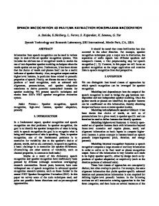
Figure 2. Full bilabial closure during the production of the words “romantic” (left) and “academic” (right).
OLR
c1
iLO
a1
OLR
3.2. Phrase recognition with multiple AF streams The second stage of our system is a word or short phrase recognizer that models visual speech in terms of the underlying articulatory processes. The recognizer uses a dynamic Bayesian network with a multi-stream structure and observations consisting of the AF classifier outputs obtained in the previous stage (see section 3.1). We will describe this framework after briefly motivating the use of multiple AF streams for visual speech recognition. The appearance of the mouth can be heavily influenced by the asynchrony between articulatory gestures. This often occurs when articulatory features not primarily involved in the production of the current sound evolve asynchronously from the ones that are. Figure 2 shows an example of such de-synchronization in two snapshots taken at the moment of complete lip closure from the utterances “romantic” and “academic”. Suppose we were to model the phoneme /m/ in these two different phonetic contexts using a single, context-independent viseme model. Both images would be considered to belong to a single class (typically the bilabial viseme) and to have the same open/closed feature value (fully closed). However, their appearance is different: in the second context, the mouth is roughly 25% wider. This is an example of contextual variation: in “romantic”, the lip rounding of /ow/ lingers during the lip closure. Thus, modeling lip rounding and lip opening as two separate articulatory features would capture more information than just modeling the /m/ viseme. Allowing the features to sometimes proceed through their trajectories asynchronously would account for these types of effects. An alternative way to model such variability is to use context-dependent units. However, visual coarticulation effects such as the one described above can span three or more visemes, requiring a large number of context-dependent models. This leads to an inefficient use of the training data, and cannot anticipate new variations. In contrast, an asynchronous AF approach offers a more flexible and parsimonious architecture. In order to take advantage of the semi-independent evolution of the AF streams–in other words, the factorization of the AF state space–we implement our model as a dynamic
c1
iLO a2
OLO
iLR
c2
a1
OLR
iLO a2
OLO
c1
c2
a2
OLO
iLD
iLD
iLD
OLD
OLD
OLD
c2
Figure 3. DBN for feature-based VSR. t is time, iF t is an index into the state sequence of feature stream F , where F ={LO,LR,LD}.
…t-1
t
t+1…
i
i
i
OVIS
OVIS
OVIS
Figure 4. Single-stream viseme HMM. i is the index into the state sequence, and O V IS is the output of the viseme classifier.
Bayesian network. Figure 3 shows three frames of the DBN used in our experiments. The model essentially consists of three parallel HMMs, one per AF, where the joint evolution of the HMM states is constrained by synchrony requirements imposed by the variables c1 and c2 . For comparison, Figure 4 shows a conventional single-stream viseme HMM, which we use as a baseline in the experimental section. Our model makes it possible for the AFs to proceed through their trajectories at different rates. This asynchrony is not completely unconstrained, however: sets of trajectories that are more “synchronous” may be more probable than less “synchronous” ones, and we impose a hard constraint on the maximum degree of asynchrony. To make the notion of asynchrony more precise, let the variable iF t be the index into the state sequence of feature stream F at time t; i.e., if stream F is in the nth state of a given word at time t, then iF t = n (see Figure 3). We define the degree of asynchrony between two feature streams F1
F2 1 and F2 at time t as |iF t − it |. The probabilities of varying degrees of asynchrony are given by the distributions of the aj variables. Each cjt variable simply checks that the degree of asynchrony between its parent feature streams is in fact equal to ajt . This is done by having the cjt variable always observed with value 1, with distribution ” “ F F P cjt =1|ajt ,it 1 ,it 2
=
1
F F |it 1 −it 2 |
=
ajt ,
⇐⇒
F2 1 and 0 otherwise, where iF t and it are the indices of the feature streams corresponding to cjt . 1 For example, for c1t , F1 = LR and F2 = LO. Rather than use hard AF classifier decisions, or probabilistic outputs as in [6] and [19], we propose to use the outputs of the decision function directly. For each stream, the observations O F are the SVM margins for that feature and the observation model is a Gaussian mixture. Also, while our previous method used viseme dictionary models [19], our current approach uses whole-word models. That is, we train a separate DBN for each phrase in the vocabulary, with iF ranging from 1 to the maximum number of states in each word. Recognition corresponds to finding the phrase whose DBN has the highest Viterbi score. To perform recognition with this model, we can use standard DBN inference algorithms [14]. All of the parameters of the distributions in the DBN, including the observation models, the per-feature state transition probabilities, and the probabilities of asynchrony between streams, are learned via maximum likelihood using the ExpectationMaximization (EM) algorithm [4].
4. Experiments In the following experiments, the LIBSVM package [3] was used to implement all SVM classifiers. The Graphical Models Toolkit [1] was used for all DBN computations. To evaluate the cascade portion of our system, we used the following datasets (summarized in Table 1). To train the lip detector, we used a subset of the AVTIMIT corpus [8], consisting of video of 20 speakers reading English sentences. We also collected our own dataset consisting of video of 3 speakers reading similar sentences (the “speech” data in Table 1). In addition, we collected data of the same three speakers making nonspeech movements with their lips (the “nonspeech” data). The latter two datasets were used to train and test the speaking-lip classifier. The “speech” dataset was manually annotated and used to train the AF and viseme classifiers. We evaluated the DBN component of the system on the task of recognizing isolated short phrases. In particular, we 1 A simpler structure, as in [12], could be used, but it would not allow for EM training of the asynchrony probabilities.
Table 1. Summary of datasets. Dataset AVTIMIT subset “speech” “nonspeech” “commands”
Description (no. of speakers) TIMIT sentences (20) TIMIT sentences (3) moving lips but not speaking (3) stereo system control commands (2)
Table 2. Stereo control commands. 1 2 3 4 5 6 7 8 9 10
“begin scanning” “browse country” “browse jazz” “browse pop” “CD player off” “CD player on” “mute the volume” “next station” “normal play” “pause play”
11 12 13 14 15 16 17 18 19 20
“shuffle play” “station one” “station two” “station four” “station five” “stop scanning” “turn down the volume” “turn off the radio” “turn on the radio” “turn up the volume”
chose a set of 20 commands that could be used to control an in-car stereo system (see Table 2). The reason “station three” is not on the list is because the subset of articulatory features we are currently using cannot distinguish it from “next station”. We collected video of two of the speakers in the “speech” dataset saying these stereo control commands (the “commands” dataset). To test the hypothesis that a DBN that allows articulator asynchrony will better account for co-articulation in faster test conditions, each command was recorded three times. The speakers clearly enunciated the phrases during the first repetition, (slow condition), then spoke successively faster during the second and third repetitions (medium and fast conditions).
4.1. Lip region localization We trained the SVM lip detector on positive examples consisting of speaking lips and negative examples taken at random locations and scales of the lower half of the face. The positive examples came from the AVTIMIT sequences, in which we hand-labeled the lip size and location. All examples were scaled to 32 by 16 pixels and corrected for illumination using simple image gradient correction. We also used a PCA transform to reduce the dimensionality of the image vector to 75 components. Unfortunately, lip detection approaches are difficult to compare, as they are not usually evaluated on the same
Table 3. Lip region localization results. Detection Rate Vertical Err. Var. Horizontal Err. Var.
Heuristic 100 % 6.8806 3.7164
AVCSR 11% 2.3930 4.8847
SVM 99% 1.4043 1.3863
dataset. The only publicly available lip tracking system, to the best of our knowledge, is the one included in the Intel AVCSR Toolkit [9]. The system starts with multi-scale face detection, then uses two classifiers (one for mouth and the other for mouth-with-beard) to detect the mouth within the lower region of the face. We compared our SVM detector with this system. To allow for a fair comparison, we recorded the face regions searched by the AVCSR detector and then searched the same regions with our detector, i.e., we used the face tracker built into the AVCSR system. For both detectors, we recorded whether lips were detected, and, if detected, their center position and scale. In addition to detection rate, we also compared position error. Table 3 shows the results for the two systems on the “speech” data, in addition to the results for the simple heuristic lip detection technique which assumes that lips are always located at a fixed position within the face region. In Table 3, “Detection rate” is the percentage of frames in which lips were detected. Since the face detection step ensured that there were always lips present in the search region, the heuristic tracker, which always gives a result, detected 100% of the lips. The AVCSR detector did poorly, only finding lips 11% of the time. Manual adjustment of the parameters of the AVCSR detector did not improve its performance. Our SVM detected lips in 99% of the frames. Since we need to extract the lip region for further processing, position error is another important performance metric. We measured position error only in the frames where lips are detected and compared the error variance, since the mean error can always be subtracted. The results show that our technique had the smallest error variances, although the heuristic did surprisingly well.
4.2. Speaking lip detection The first step of our two-step speech detection process is to determine whether the lips are moving. This is done by first calculating normalized image difference energy in consecutive frames, then low-pass filtering the image energy over a one-second window (with a 2 Hz cut-off frequency). A threshold is applied to this filtered output to determine whether the lips are moving. For now, this threshold is manually chosen to give reasonable performance, but we hope to use a more principled approach in the future.
(a) Speaking
(b) Nonspeaking
Figure 5. Sample frames of speaking and nonspeaking lips.
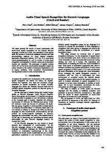
The second step determines whether the lip configuration is consistent with speech activity using an SVM classifier. This classifier is only applied to frames which were classified as moving in the first step. Its output is median filtered using a half-second window to remove outliers. We train the SVM classifier on the lip samples detected in the “speech” and “nonspeech” datasets. Figure 5 shows some sample lip detections for both speaking and nonspeaking sequences. Lips were detected in nearly 100% of the speaking frames but only in 80% of the nonspeaking frames. This is a positive result, since we are not interested in nonspeaking lips. The 80% of nonspeaking detections were used as negative samples for the speaking-lip classifier. We randomly selected three quarters of the data for training and used the rest for testing. Figure 6 shows the ROC for this second step, generated by sweeping the bias on the SVM. Setting the bias to the value learned in training, we achieve 98.2% detection and 1.8% false alarm. Figure 7 shows the result of our two-step speech detection process on a sequence of stereo control commands, superimposed on a spectrogram of the speech audio to show that our segmentation is accurate. We only miss one utterance and one inter-utterance pause in this sample sequence.
4.3. AF classification SVM classifiers for the three articulatory features were trained on the “speech” dataset. To evaluate the viseme baseline, we also trained a viseme SVM classifier on the same data. The mapping between the six visemes and the AF values they correspond to is shown in Table 4. There are two reasons for choosing this particular set of visemes. First, although we could use more visemes (and AFs) in principle, these are sufficient to differentiate between the phrases in our test vocabulary. Also, these visemes correspond to the combinations of AF values that occur in the training data, so we feel that it is a fair comparison. We
Frequency
8000 6000 4000 2000 0 0
5
10
15
Time
20
25
30
Figure 7. Segmentation of a 30-second sample sequence of stereo control commands. The black line is the output of the speaking vs. nonspeaking detection process. The line is high when speaking lips are detected and low otherwise. The detection result is superimposed on a spectrogram of the speech audio (which was never used by the system).
Pr(detection)
1
Table 4. The mapping from visemes to AFs. Viseme 1 2 3 4 5 6
0.95 0.9 0.85 0
0.05 Pr(false alarm)
LO closed any narrow medium medium wide
LR any any rounded unrounded rounded any
LD no yes no any any any
0.1
Figure 6. Speaking vs. nonspeaking ROC. The y-axis shows the probability of detecting speaking lips when they are present. The x-axis shows the probability of incorrectly detecting speaking lips when they are not present.
used the one-vs.-all multi-class SVM formulation, training a total of six SVM classifiers for the three AFs: four SVMs for LO, one for LR, and one for LD; and one SVM for each of the six visemes. Thus, for both the AF DBN and the viseme HMM, the observations in each frame consisted of six decision values. The input vectors for the SVMs were produced by first resizing the mouth regions to 32 by 16 pixels, and then applying a discrete cosine transform (DCT) to each image to obtain a set of 512 coefficients. The dimensionality was further reduced using a PCA transform, with the top 75 PCA coefficients retained as the final observation vector. Radial
Table 5. Classifier accuracies for the feature and viseme SVMs. Accuracy
LO 79.0%
LR 77.9%
LD 57.0%
viseme 63.0%
basis function (RBF) kernels were found to produce the best results. The error term penalty parameter C and the γ parameter of the RBF were optimized using four-fold crossvalidation on the training set. In order to evaluate the performance of the classifiers, we labeled a subset of the “commands” data corresponding to one speaker with AF and viseme labels. Table 5 shows the classifier accuracies on this testPset, averaged over N the N classes for each SVM: acc = N1 i=1 acc(class i). 1 Chance performance is N . The numbers of classes are: 4 for LO, 2 for LR and LD, and 6 for the viseme SVM. Note that the labio-dental SVM has lower performance than the lip-opening and lip-rounding SVMs, possibly due to limited training data, as there were very few instances of /f/ and /v/ in the dataset.
Table 6. Number of phrases (out of 40) recognized correctly by various models. The first column lists the speed conditions used to train and test the model. The next three columns show results for dictionary-based models. The last three columns show results for whole-word models. train/test slow-med/fast slow-fast/med med-fast/slow average average %
viseme+GM 10 13 14 12.3 30.8
dictionary-based feature+SE feature+GM 7 13 13 21 21 18 13.7 17.3 34.2 43.3
4.4. Phrase recognition In this section, we evaluate our phrase recognizer on the stereo control command task and compare its performance to several baseline models. The experimental setup is as follows. Recall that the two speakers repeated each stereo control command at slow, medium and fast speeds. We run each experiment three times, training the system on two speed conditions and testing it on the remaining condition. We then average the accuracies over the three trials. The rightmost three columns of Table 6 (labeled wholeword) compare our AF-based DBN model to the visemebased HMM baseline (shown in Figure 4). The baseline, referred to as viseme+GM, uses the six decision values of the viseme SVMs as observations. We evaluate two versions of our AF-based model: one with strict synchrony enforced between the feature streams, i.e. aj = 0 (feature+GM), and one with some asynchrony allowed between the streams (async feature+GM). In the model with asynchrony, the LR and LO feature streams are allowed to de-synchronize by up to one index value (one state), as are LO and LD. The two asynchrony probabilities, p(a1 = 1) and p(a2 = 1), are learned from the training data. All three of the above systems use whole-word units and Gaussian mixture models (GMs) of observations (in this case, single Gaussians with tied diagonal covariance matrices). The results show that, on average, using AF classifiers is preferable over using viseme classifiers, and that allowing the AF streams to de-synchronize can further improve performance. Looking at each of the train and test conditions in more detail, we see that, when the training set includes the slow condition, the asynchronous AF model outperforms the synchronous one, which, in turn, outperforms the viseme baseline. (The McNemar significance levels p [21] for these differences are shown in the table). However, when the models are trained on faster speech and tested on slow speech, the baseline does better than the AF models. This suggests that our approach is better at accounting for variation in speech
viseme+GM 16 19 27 20.7 51.6
whole-word feature+GM async feature+GM 23 (p=0.118) 25 (p=0.049) 29 (p=0.030) 30 (p=0.019) 25 24 25.7 26.3 64.1 65.8
that is faster than the speech used for training. The leftmost three columns of the table correspond to three dictionary-based models. Rather than use whole-word recognition units, these systems use a dictionary that maps phrases to sequences of contextindependent phoneme-sized units—an approach used for large-vocabulary tasks and one that we have used previously [19]. In particular, the dictionary-based feature+SE model is the multi-stream AF DBN presented in [19]. Instead of training Gaussians over the SVM scores, it converts SVM scores to scaled likelihoods, which it uses as soft evidence (SE) in the DBN. Note that, while in [19] the DBN parameters were set manually, here we learn them from training data. The results show that both of our proposed AF models perform much better on this task than does the feature+SE model. To evaluate the relative importance of the differences between the models, we modify the feature+SE baseline to use single Gaussians with diagonal covariance over SVM scores, instead of converting the scores to scaled likelihoods. The resulting feature+GM model is still dictionary-based, however. We can see that, while this improves performance over using soft evidence, it is still preferable to use whole-word models for this task. Finally, we evaluate a dictionary-based version of the viseme HMM baseline, viseme+GM. The results indicate that, as was the case for whole-word models, using AF classifiers is preferable over using viseme classifiers.
5. Summary and conclusions In this paper, we have proposed an architecture for visual speech detection and recognition. We have shown that a discriminative cascade achieves robust lip detection results, improving significantly upon the baseline performance of previous methods. It also offers accurate discrimination between speaking and nonspeaking lip images and classification of distinctive articulatory features. For phrase recognition, we have proposed a DBN with loosely coupled streams
of articulatory features, where the observation model is a Gaussian mixture over the feature classifier outputs. This approach can naturally capture many of the effects of coarticulation during speech production. In particular, our results suggest that it can better account for variation introduced by speech which was spoken more quickly than that in the training data. We have also compared wholephrase models to dictionary-based models, and the Gaussian mixture-based observation model to one with classifier outputs converted to soft evidence. We have found that, on a real-world command recognition task, whole-word models outperform dictionary-based ones and Gaussian mixturebased observation models outperform soft evidence-based ones. For the purposes of quick implementation, this work has used a limited feature set containing only the features pertaining to the lips. Future work will investigate more complete feature sets, and compare the approach against using other types of visual observations, such as appearancebased features. We will also focus on evaluating our system on larger multi-speaker datasets, a wider variety of phrases, and more subtle nonspeech events.
Acknowledgments This research was supported by DARPA under SRI subcontract No. 03-000215.
References [1] J. Bilmes and G. Zweig, “The Graphical Models Toolkit: An open source software system for speech and time-series processing,” in Proc. ICASSP, 2002. [2] M. Brand, N. Oliver, and A. Pentland, “Coupled hidden Markov models for complex action recognition,” in Proc. IEEE International Conference on Computer Vision and Pattern Recognition, 1997. [3] C. Chang and C. Lin, “LIBSVM: A library for support vector machines,” 2001. Software available at http://www.csie.ntu.edu.tw/˜cjlin/libsvm. [4] A. Dempster, N. Laird, and D. Rubin, “Maximum likelihood from incomplete data via the EM algorithm,” Journal of the Royal Statistical Society, 39:1–38,1977. [5] Z. Ghahramani and M. Jordan, “Factorial hidden Markov models,” in Proc. Conf. Advances in Neural Information Processing Systems, 1995. [6] M. Gordan, C. Kotropoulos, and I. Pitas, “A support vector machine-based dynamic network for visual speech recognition applications,” in EURASIP Journal on Applied Signal Processing, 2002.
[7] G. Gravier, G. Potamianos, and C. Neti, “Asynchrony modeling for audio-visual speech recognition,” in Proc. HLT, 2002. [8] T. Hazen, K. Saenko, C. H. La, and J. Glass, “A segment-based audio-visual speech recognizer: Data collection, development, and initial experiments,” in Proc. ICMI, 2005. [9] Intel’s AVCSR Toolkit source code can be downloaded from http://sourceforge.net/projects/opencvlibrary/. [10] S. King, T. Stephenson, S. Isard, P. Taylor and A. Strachan, “Speech recognition via phonetically featured syllables,” in Proc. ICSLP, 1998. [11] K. Kirchhoff, “Robust Speech Recognition Using Articulatory Information,” PhD thesis, University of Bielefeld, Germany, 1999. [12] K. Livescu and J. Glass, “Feature-based pronunciation modeling for speech recognition,” in Proc. HLT/NAACL, 2004. [13] J. Luettin, “Towards speaker independent continuous speechreading,” in Proc. European Conference on Speech Communication and Technology, 1997. [14] K. Murphy, Dynamic Bayesian networks: representation, inference and learning. Ph.D. thesis, U.C. Berkeley CS Division, 2002. [15] C. Neti, G. Potamianos, J. Luettin, I. Matthews, H. Glotin, and D. Vergyri, “Large-vocabulary audiovisual speech recognition: A summary of the Johns Hopkins Summer 2000 Workshop,” in Proc. Works. Signal Processing, 2001. [16] H. Nock and S. Young, “Loosely-Coupled HMMs for ASR,” in Proc. ICSLP, 2000. [17] G. Potamianos, C. Neti, G. Gravier, A. Garg, and A. Senior, “Recent advances in the automatic recognition of audio-visual speech”, in Proc. IEEE, 2003. [18] K. Saenko, J. Glass, and T. Darrell, “Articulatory features for robust visual speech recognition,” in Proc. ICMI, 2005. [19] K. Saenko, K. Livescu, J. Glass, and T. Darrell, “Production domain modeling of pronunciation for visual speech recognition,” in Proc. ICASSP, 2005. [20] Y. Zhang, Q. Diao, S. Huang, W. Hu, C. Bartels, and J. Bilmes, “DBN based multi-stream models for audiovisual speech recognition ”, in Proc. ICASSP, 2004. [21] http://www.nist.gov/speech/tests/sigtests/mcnemar.htm.