Online simulations http://laurent.perrinet.free.fr/code/visual.html. References. 1. Joseph J. Atick and A. Norman Redlich. What does the retina know about natural ...
Visual Spike Coding Using a Statistically Optimized Overcomplete Representation Laurent Perrinet and Manuel Samuelides ONERA/DTIM, 2, av. Belin, 31055 Toulouse, France
Abstract. In order to explore visual coding strategies, we use a wavelet-like transform which output is sparse, as is observed in the primary visual areas [6]. This transform is defined in the context of a feed-forward spiking neural network, and the output is the list of its neurons’ spikes: it is recursively constructed using a greedy matching pursuit scheme which first selects best matches and then laterally interacts with its correlated neighbors. We study the quality of this algorithm and its enhancement by the prior knowledge of the statistics of its input, namely natural images. An application to image compression is shown which is comparable to other techniques such as JPEG at low bit compression.
1 Introduction 1.1 What is the goal of visual coding? Faced with the light influx from the outside world, what are the plausible strategies to extract the relevant features necessary to a given goal? The physiology of the neurons, the architecture of the visual system and the statistics of the light inputs are as many constraints on the visual system, and a key challenge is to ”break” the code of vision. As was proposed by D. Marr [5] a primary stage is to construct a ”primal sketch” of the image as a combination of edges at different scales, but it is still uncertain how this may be built. Among proposed strategies, dimension reduction (PCA), blind source separation (e.g. ICA) and sparse coding [6] are the most successful. This last method suggests that the code could consist of a relatively small number of active spiking neurons if their spatial weighting functions form an overcomplete basis of the input space. But this fails so far to use the temporal aspect of neuronal processing. In fact, this aspect seems crucial and recently, ultra rapid categorization [8] was shown in humans and monkeys and urged the computational neuroscience community to explore new coding strategies accounting for the consequences of those experiences. To gain advantage over the speed of retinal processing, the code should convert the analog intensities into a ’wave’ of spikes in less than 20 ms, the most ’important’ spikes being fired first. This defines a new goal for the retinal code: the analog image should be temporally transformed so that the spike list transmits progressively the most information with the shortest latency.
1.2 Primary visual image processing The primates’ primary visual system consists in different neuronal layers from the retina through the Lateral Geniculate Nucleus (LGN) and to V1. In this study, these complex intertwined sub-systems are roughly simplified as a one-pass feed-forward layer of spiking neurons that would transform the image into a pattern of spikes. This algorithm is quite general and will constitute a conceptual construction framework for us and may be extended to multiple layers. We may describe the linear characteristics of the neurons of this layer by spatial kernels. Their receptive fields (RFs) are localized and overlapping and their sizes are generally non-uniformly distributed over the visual field. They are bandpass and some are oriented. These neurons are observed in numerous biological systems since the seminal work of Hubel [3], but also emerge from self organized systems constrained under ecological constraints [6]. Each neuron integrates this information at his soma until it reaches a threshold: it then emits a spike. The image code consists exactly on the spiking times (or latencies) for the different fibers and practically, the latency of spike emission is inversely proportional to the correlation of the input with the kernel. 1.3 Definition of the article’s framework Following [6], we assume that an approximation If of an image I may be calculated as the linear sum of different ’patches’ from a given dictionary D of spatial weighting functions φi : X ai φi (1) If = i∈D
Minimizing kI − If k leads to a combinatorial explosion of the freedom of choice of the subset of D and of the values ai (it is a NP hard problem [4]). In this article, after defining our model, we apply it to the framework of the experiences of Thorpe et al. [8] and finally study the influence of introducing a prior knowledge of the inputs’ statistics. Also, to illustrate the performance of our coding strategy, we apply our results to a compression application : after building a simple reconstruction scheme, the code may be compared to other models -as the popular JPEG format- by its reconstruction quality according to the compression rate.
2 Description of the visual model 2.1 Response of the neuronal layer Generally, we write as in [1] the output of the linear layer: X Ci =< I, φi >= I(l).φi (l) l∈Ri
(2)
where I(l) is the light intensity at pixel l and Ri is the receptive field (i.e support) of φi . The dictionary should consist of independent components of the input space, and following the work of Bell et al. [2], we define the weight vectors φi of the neurons as
dilated, translated and sampled Mexican Hat (or DOG) and Gabor filters (see [4, pp. 77, 160]). A neuron will be totally characterized by the triplet i = (σ, λ, θ) where θ is the neuron’s orientation (set to N U LL for the DOG). For simplicity and given our application’s goal, we will define the cells’ RFs by different scales σ and distribute the neurons’ localizations λ uniformly on a rectangular grid for each scale. The grid’s spacing is set proportionally to σ so that the subsampled neuronal layer fill uniformly the spatial/frequency space. The norm of the vectors φi are Ni := kφi k. 2.2 Propagation algorithm and lateral interactions Let’s initially set I 0 := I and Ci0 := Ci . First, we determine the first neuron in the layer to fire: i0 = ArgMaxi (|Ci0 |) (3) and for this index i0 = (σ 0 , λ0 , θ0 ), we define the extremal contrast value C0 (i0 ). Actually, we found the best match in the sense of the projection on our basis, so we use a projection pursuit scheme, i.e. we subtract the projection from I 0 : I1 = I0 −
φ0 < I 0 , φi0 > φi0 = I 0 − Ci00 i 2 2 kφi0 k Ni0
(4)
The contrast becomes Ci1 =< I 1 , φi >= Ci0 − Ci00
< φi0 , φi > Ni0 2
(5)
Iterating this steps in time, our algorithm is simply for t ≥ 0, given the initialization: it = ArgMaxi∈D (|Cit |) < φ it , φ i > Cit+1 = Cit − pt .mt Nit 2 with mt = |Citt | and pt is the sign of Citt (i.e. its ON or OFF polarity). This algorithm is exactly similar to [4, pp.412–419] for normalized filters (Ni = 1) under the term Matching Pursuit (MP).The image code is given by the list (it , pt , mt ) of the spikes’ order with their corresponding value of polarity and extremal contrast value. Finally the algorithm is stopped at time tf when the absolute contrast is less than a given threshold. To reconstruct the image we derive immediately I=
tf X
pt .mt
t=1
φit + I tf Nit 2
(6)
which was our goal in (Eq. 1). 2.3 Sparse coding of the visual input It is interesting to see that once a match is chosen, its correlated activity is substracted. It is in accordance with our goal of finding the independent sources of each image but
also with neurophysiological data which show that a suggested role for lateral connections in a neuronal layer is to lower activity correlations. Mathematically, a convergence theorem is available: the error decreases monotonically and exponentially to 0 when t tends to infinity (see proof in [4, p.414] and Fig. 2 - A,B). This result is essential in the context of visual coding since it means that all the information will be stored in a few active spiking neurons. We applied our method to different 128x128 images and, as in [4], √ we define Ni = 1 for each scale. The scale grows geometrically with a factor ρ = 5 2 (i.e. 5 layers per octave) on 41 scales and the direction is circularly N U LL, 0, π/4, π/2 and 3π/4. We may easily compute the maximum number of bytes necessary to describe the spike list as I = nspike × log2 (nneurons × nquantize )/8 where nquantize is the number of quantization levels for the contrast (here 128). Moreover, if npixel is the number of pixels in npixels the image, nneurons = 1−ρ −2 . Numerically, the information rate is in this simulation ∼ 2.88 byte/spike. As in [9], the recoded image is recognizable after only a few spikes (Fig. 1-B) and convergence is fast as of the Mean Square Error (MSE) (see Fig. 2 - A,B). This coding strategy provides a sparse representation of the signal: in comparison with the dyadic decomposition [9], the output coefficients and the MSE decrease more rapidly to 0 since correlated activity is removed. It transmits most active spikes first, and leads therefore to very good information transfer rate even on very short latencies.
A
B
D
E
Fig. 1. Different reconstruction of Lena for a given file size of 2000 bytes. (A) Detail of the original 128x128 image; reconstruction using (B) Matching Pursuit; (C) Whitened MP; and in comparison with (D) JPEG (Quality 32)
3 Whitened Matching Pursuit 3.1 Whitening of the images’ power spectrum using natural images statistic Experimental data on natural images show that their spatial power spectrum obey to some invariants [1] that are mainly related to their property of scale invariance. Therefore, we may find a priori a whitening filter K so that the images would be decorrelated across spatial frequencies, and up to a critical frequency determined by the noise. Experimentally, we used the method of Atick et al. [1] on a set of natural images taken from natural outdoor images used in [8] having no striking statistical particularities (like
a wide open sky or excessive contrast of the sun through leaves) to calculate the mean spatial cross-correlation. The bandpass filter is set experimentally with a cutting frequency of f0 = 200 cycles/picture. The resulting whitening filter is similar to [1] and enhances mostly high frequencies. Practically, the whitened images are uncorrelated: first and second order statistics are removed. The whitening lets higher order statistics clearly appear. We integrate this strategy into the MP algorithm by using whitened filters ψi computed from the normalized filters with: ψi = φ i ∗ K
(7)
This Whitened Matching Pursuit (WMP) strategy is less ”greedy” with respect to Mean Squared Error (MSE) (Fig. 2 - A), and its quality may be captured by a Malhanobis ponderation of the MSE: the metric is computed through a filtered covariance matrix of the image database, which amounts of the convolution with K (see Fig. 2 - B). This measure should be compared with subjective image appreciation, since human vision is more sensitive to high frequency errors. 3.2 Numerical results We applied this method with the same protocol as in 2.3. The reconstruction is similar (see Fig. 1 - C), but with finer details. Numerically, we observed that WMP didn’t reached a plateau as soon as MP, and this may be interpreted by the fact that WMP catches edges independently of their scale and therefore follows the structure of the image. A toy simulation with an image presenting the same object at two scales revealed that MP decomposed the bigger one first, whereas WMP decomposed the 2 objects independently, which is similar to most visual goal, since it is important for instance to recognize objects by their saliency and not by their scale. We also observed that using
A
MP
WMP
Jpeg
B
C
0
10
WMP
WMP
−1
MP
10
MP Jpeg 1000 2000 3000
1000 2000 3000
200
600
1200
Fig. 2. (A,B) Comparison of MSE in function of the file size (in bytes) and compared to JPEG at different qualities (dashed line: MP, plain line: WMP, dotted line: JPEG) (A) Standard MSE, (B) Whitened MSE; (C) Modulation function for MP and WMP in function of the spike’s rank. WMP, the spikes’ firing become more independent in function of their rank, i.e. their
importance: this strategy maximizes the entropy of the output spike order distribution and enhances information transfer since it reduces redundancy. If its convergence is better, a drawback of WMP is the slower decay of the modulation. This means that the representation of the image is less sparse (in fact the kurtosis of pt .mt drops from ∼ 42.1 to ∼ 1.52). This is partly due to the excessive greediness of MP but also to the suboptimal choice of the filters, as these should be learned from the image database.
Conclusion We have proved that we may define a code based on a dictionary of primary visual weight vectors and that this code is efficient and sparse. We also shown that tuning the frequency sensibility according to the statistics of the natural images leads to a very efficient coding strategy which compares at high compression ratios to image processing standards like JPEG and that this may be used by the retina especially for low bit compression and fast image transmission. Moreover, it has been shown [7,9] that the modulation function obey to invariances: it can be only given by its polarity (ON or OFF) and the spike rank, decreasing the quantization to 2 and thus improving the compression rate. Its biological plausibility and high performance demonstrate that a model combining overcomplete representation and temporal processes may be crucial in the understanding of the visual system. This work is therefore a first step before the implementation of the algorithm to a set of layers (from the retina to layer V1 and V2) and also to V4 and MT layers with more ’abstract’ dictionaries. Online simulations http://laurent.perrinet.free.fr/code/visual.html
References 1. Joseph J. Atick and A. Norman Redlich. What does the retina know about natural scenes? Neural Computation, 4(2):196–210, 1992. 2. Anthony J. Bell and Terrence J. Sejnowski. The ‘independent components’ of natural scenes are edge filters. Vision Research, 37(23):3327–3338, 1997. 3. D.H. Hubel and T.N Wiesel. Receptive fields of single neurones in the cat’s striate cortex. Journal of Physiology, 148:574–591, 1959. 4. St´ephane Mallat. A Wavelet Tour of signal Processing. Academic Press, 1998. 5. David Marr. Vision. W. H. Freeman and Co., 1982. 6. Bruno A. Olshausen and David J. Field. Sparse coding with an overcomplete basis set: A strategy employed by v1? Vision Research, 37:3311–3325, 1998. 7. Laurent Perrinet and Manuel Samuelides. Sparse image coding using an asynchronous spiking neural network. In Proceedings of ESANN, 2002. 8. Simon J. Thorpe, Denis Fize, and Catherine Marlot. Speed of processing in the human visual system. 381, pages 520–522, 1996. 9. Rufin Van Rullen and Simon J. Thorpe. Rate coding versus temporal order coding: What the retina ganglion cells tell the visual cortex. Neural Computation, 13(6):1255–1283, 2001.