Visual Understanding via Multi-Feature Jointly Sharing Learning Lei Zhang, Member, IEEE, and David Zhang, Fellow, IEEE Abstract—Image/video data is usually represented by multiple visual features. Fusion of multi-sources information for establishing the identity has been widely recognized. Multi-feature visual recognition has recently received attention in multimedia applications. This paper studies visual understanding via a newly proposed -norm based multi-feature jointly sharing learning framework, which can simultaneously learn the global label matrix and explicit classifiers from the labeled visual data represented by multiple feature modalities. Additionally, a multi-modal group graph manifold regularizer formed by mixed Laplacian and Hessian graph is proposed for better preserving the manifold structure of different features on the labeled data, while preserving the label consistency and improving the label prediction power via semi-supervised learning. The merits of the proposed multi-feature learning framework lie in jointly sharing the structural information from multiple features in global classifier learning phase based on a mixed graph regularizer on one hand, and an efficient alternating optimization method for fast classifier training on the other hand. Experiments on several benchmark visual datasets, such as 17-category Oxford Flower dataset, the challenging 101-category Caltech dataset, YouTube & Consumer Videos dataset and large-scale NUS-WIDE dataset for multimedia understanding all demonstrate that the proposed approach compares favorably with state-of-the-art algorithms. Index Terms—Visual recognition, multimedia understanding, sharing learning, multi-feature learning, semi-supervised learning
I. INTRODUCTION ulti-modality, multiple views and multiple features are usually used to represent multimedia content and images. For example, given a face image or a video frame, its visual content can be represented by several kinds of weak modalities such as left and right periocular, mouth and nose regions [4] for robust face recognition, or different feature types such as histogram, SIFT, HSV, etc. [9] for action recognition. It therefore becomes a challenging task in multimedia analysis for improving the visual classification performance by simultaneously sharing the structural information from multiple information sources of independent or correlated feature representations.
M
L.
Zhang is with the College of Communication Engineering, Chongqing University and the Department of Computing, The Hong Kong Polytechnic University, Hong Kong (e-mail:
[email protected]). D. Zhang is with the Department of Computing, The Hong Kong Polytechnic University, Hong Kong (e-mail:
[email protected]).
In early, information fusion can be done at three levels: feature level, score level and decision level, whereas feature level fusion can be more discriminative than other two level-fusions [16]. Feature concatenation is a prevalent fusion method which has been used in patter recognition [18], [19]. However, it is less effective in multimedia content analysis, especially when the features are independent or heterogeneous [17], and in particular, simple feature concatenation for high dimensional feature vectors may also become inefficient and non-robust. Therefore, multi-view learning and multiple kernel learning have been developed by researchers in machine learning community to address this problem. One popular work is the two-view based support vector machine (SVM-2k) [11], [21], [22], which jointly learns SVM with two views. Another popular work is multiple kernel learning (MKL) [10], [20], which focus on the information integration from multiple features by combining multiple kernels with respective weights. Besides, the concept of multi-modal joint learning was also involved in dictionary learning and sparse representation. Some representative works under the framework of dictionary learning such as [25], [26], [27], [28], [29] have been proposed for visual recognition including face, digit, action, and object recognition, which demonstrate that training more discriminative dictionaries and jointly learning visually correlated dictionaries can effectively improve the recognition performance of the reconstruction based classifier proposed in [24]. Also, several multi-modal joint sparse representation methods were developed for face and visual recognition applications. For examples, in [3], a multi-task joint sparse representation classifier (MTJSRC) was proposed for visual classification in which group sparsity was used to combine multiple features. In [4], a multimodal joint sparse representation and kernel space multimodal sparse model were proposed for robust face recognition. In [30], a joint dynamic sparse representation classifier model was proposed for object recognition. In [48], a very efficient multi-task feature selection model (FSSI) with information sharing in low-rank solution was proposed for multimedia analysis. Though these multi-task/multi-view based joint learning performs better than single modality, they depend on sufficient labeled data that may conflict with real-world applications. Therefore, we focus on a semi-supervised learning mechanism that can improve the robustness of learned classifier when label information of training samples is insufficient. It’s known that among semi-supervised learning methods, manifold regularization, specifically, Laplacian graph regularization
learning becomes the main stream for well exploring the geometry of the intrinsic data. Although Laplacian graph achieves good performance, it has been identified to be biased towards a constant function due to its constant null space and the not well preserved local topology, especially when there are only few labeled data. Comparatively, Hessian regularization has better extrapolating power shown in two facets [5]: first, it has a richer null space and second, it can exploit the intrinsic local geometry of the data manifold very well. For better Videos
exploitation of multiple features in classifier learning, excited by spirits of these joint learning concepts discussed above, we consider a more intuitive manner, i.e. multi-feature global label consistency based classifier learning under a mixed Hessian and Laplacian regularization based semi-supervised framework. It’s worth noting that there is no explicit mapping matrix in manifold regression during testing process, therefore, in this work, we will simultaneously learn an explicit global classifier.
Flowers
Object images in Caltech
Video/Image Training Data
Multiple Low-level Features
Low-level features= {SIFT, ST}|L=0,1 X={X1, X2, X3, X4}|m=4
Low-level features = {Color, Shape, Texture, HSV, HOG, SIFTint, SIFTbdy} X={X1, X2, …, X7}|m=7
Video/Image Testing Data
Low-level features = {PHOW-gray, PHOW-color, SSIM, GB} X={X1, X2, X3, X4}|m=4
Robust Classifier Learning
Fig. 1. Overview of the proposed framework. The algorithm exploits a jointly sharing learning over multiple visual feature modalities. Finally, a multimodal joint recognition is done through the learned robust classifiers.
Motivated by these above concerns, a multi-feature group graph regularizer by jointly learning mixed Laplacian and Hessian regularization is proposed for visual categorization. We uniformly name the proposed algorithm as multi-feature sharing based Global Label Consistent Classifier framework (GLCC). The merits of this paper are shown as follows. Multiple feature modalities are jointly learned with effective knowledge and feature structure sharing for robust visual classification. To better preserve the manifold structure of training data, a multi-modal group graph regularizer based on Hessian and Laplacian regularization is presented for label consistency preservation. Considering that there is no explicit classifier in manifold regression, an explicit classifier for global label prediction is simultaneously learned by minimizing the weighted least square loss with global label prediction. In the proposed method, a -norm based global classifier solved with a very efficient alternating optimization in low computational cost is presented. The overview of the proposed GLCC framework is illustrated in Fig.1. The visual experiments have been conducted on the benchmark visual datasets, including the Oxford flower 17 dataset1 from [12], the Caltech 101 dataset2
from [14], the YouTube & Consumer video dataset3 from [45], and the large scale real-world NUS-WIDE web image dataset4 from [53] for multimedia analysis. All experiments demonstrate that our GLCC method outperforms many existing multi-feature and semi-supervised learning methods. The rest of this paper is organized as follows. In section II, we review the most related works in visual recognition and multi-view graph based learning. The proposed -norm based multi-feature global label consistent classifier framework including its formulation and training algorithm is described in section III. The experiments on several benchmark datasets for visual application are employed in Section IV. The convergence and computational time analysis is briefly discussed in section V. Section VI concludes this paper. II. RELATED WORKS As discussed previously, this work is closely related to the efforts on visual recognition and multi-modal graph based learning. In this section, we will briefly review the current prevailing approaches.
3 1
http://www.robots.ox.ac.uk/~vgg/data/flowers/17/index.html 2 http://www.robots.ox.ac.uk/~vgg/software/MKL/
http://vc.sce.ntu.edu.sg/transfer learning domain adaptation home.html 4 http://lms.comp.nus.edu.sg/research/NUS-WIDE.html
adaptation/domain
A. Visual Recognition A number of methods have been developed for visual recognition, such as face recognition, gender recognition, age estimation, scene categories and object recognition in computer vision community. The bag-of-features (BoF) model has been a popular image categorization, but it discards the spatial order of local descriptors which limits the descriptive power of the image representation. In [2], a spatial pyramid matching (SPM) beyond bags of features was proposed for natural scene categories and object recognition. Yang et al. [40] also proposed a linear SPM based on sparse coding (ScSPM) for visual classification and obtained significant improvement. In [1], Gehler et al described several feature combination methods including average kernel support vector machine (AK-SVM), product kernel support vector machine (PK-SVM), multiple kernel learning (MKL) [23], [37], [38], column generation boosting (CG-Boost) [13], and linear programming boosting (LP-B and LP-β) [15] for object recognition. However, the common flaw of these methods is their large computational cost. Recently, Yuan et al. [3] proposed a multi-task joint sparse representation (MTJSRC) using mixed-norm for visual classification, and obtained better performance by comparing with several sparse dictionary learning methods [24], [25], [26], [27], [28]. Zhang et al. [30] proposed a multi-observation joint dynamic sparse representation for visual recognition, and obtain comparable performance. All these works demonstrate that multi-feature joint learning has a positive effect on robust classifier learning for visual understanding. B. Graph based Semi-supervised Learning Semi-supervised learning has been widely deployed in the recognition task, due to the fact that training a small amount of labeled data is prone to overfitting, while manual labeling of a large amount of precisely labeled data is tedious and time-consuming. Most related to the paper, a subspace sharing based semi-supervised multiple feature analysis method for action recognition was proposed [8], in which both the global and local structural consistency has been considered in discriminative classifier training. Zhou et al. [31] proposed a graph based semi-supervised method (LGC) for learning local and global consistency by a regularization framework. In [7], a Laplacian graph manifold based semi-supervised learning was proposed, in which a manifold assumption that the manifold structure information of the unlabeled data can be preserved was given. The assumption of consistency means that the nearby points are likely to have the same label and the points on the same cluster/manifold are likely to have the same label. Note that cluster assumption is local while manifold assumption is global. In [51], a semi-supervised feature selection algorithm SFSS for multimedia analysis based on Laplacian graph and l2,1-norm regularization was proposed. Graph manifold based algorithms make use only of the nearest neighbor information to classify the unlabeled data. Laplacian eighenmap based manifold learning was usually proposed for dimension reduction and graph embedding [6], [32], [33], [34], but all of them were implemented in single view/modality. In [36], a graph Laplacian based multi-view spectral embedding
(MSE) method was proposed for dimension reduction. Recently, Yang et al. [9] proposed a multi-feature Laplacian graph based hierarchical semi-supervised regression (MLHR) for multimedia analysis and achieved better performance in video concept annotation. Throughout these manifold based methods presented above, Laplacian graph and single feature are the mainstream of semi-supervised learning, however, it has been identified in [5] that it suffers from the fact that the solution is biased towards a constant with weaker extrapolating power. Hessian graph exploited for semi-supervised dimension reduction [5] was proved to have a good extrapolating power. Therefore, this paper further explores a multi-feature joint learning framework into which Hessian regularization is incorporated for global label consistent classifier learning. C. Multi-view Graph based Learning Multi-view graph manifold regression has been reported in recent years. Belkin et al. [41] proposed a manifold regularization framework for semi-supervised learning. Laplacian regularized least square and Laplacian support vector machine have been discussed in their work, but in single view. Tong et al. [42] proposed a graph based multi-modality learning method with linear and sequential fusion schemes, but the mapping function in the objective function is implicit. Xia et al. [35] proposed a multi-view graph embedding which calculates an eigenvalue problem in optimization, but for dimension reduction. Wu et al. [43] proposed a sparse multi-modal dictionaries learning with Laplacian hyper-graph as regularization. Wang et al. [8] proposed a semi-supervised multiple feature learning framework in which graph Laplacian regularizer and subspace sharing were studied for action recognition. Therefore, under the multi-view learning and graph manifold, an idea of multi-modal global label consistent classifier is verified in this work. III. MULTI-FEATURE GLOBAL LABEL CONSISTENT CLASSIFIER In this section, the -norm based GLCC framework with model formulation, optimization, training algorithm, and recognition is presented. A. Notations Assume that there are n training samples with d-dimensional vector from c classes. Denote as the training set of the i-th feature modality, as the global label information of the training samples with c classes, and as the predicted label matrix of training data. di denotes the dimension. In this paper, and denote Frobenius norm and -norm, Tr(·) denotes trace operator. Given a sample vector xi, if xi belongs to the j-th class, and , otherwise. The learned classifier of the i-th feature is parameterized as with a bias . The Laplacian and Hessian graph matrix are represented to be and , respectively. B. Formulation of GLCC Semi-supervised learning approach holds the assumption
that nearby points are more likely to have the same labels. In graph based manifold learning, label consistency is embedded in data manifold structure. Inspired by [8], [35], [41], [42], [43], the multi-feature GLCC is generally formulated as follows.
details of Hessian energy estimation and the computation of Hessian energy matrix are shown in Appendix A. Therefore, for exploiting the advantages of both regularizers, the manifold regression model with group graph regularizers can be represented as
(1)
(7)
where γ and λ are positive trade-off parameters, is a full one vector, F is the global prediction, is a loss function, and is a graph manifold preservation term. For convenient analysis, let , the objective function of graph based manifold regression model can then be written as (2) where denotes the least square loss function used in this work, is a regularization parameter ( ), and denotes the adjacency matrix defined as (3) where denotes the local set represented by k-nearest neighbors of xj. The least square loss term of (2) is considered as a weighted loss function here, which can be written as
(4) where denotes trace operator, and W is a diagonal matrix with entries Wii defined as follows: for semi-supervised use, Wii is set as a large value (e.g. 1010) if the i-th sample is labeled, and 0 otherwise. The second term of (2) is a manifold structure preservation term for exploring label consistency. Specifically, Laplacian graph is used in part to preserve the label information in the manifold built on the training data. It can be written in trace-form as (5) where
is a diagonal matrix with entries , and is Laplacian graph matrix. As denoted in [5], the graph Laplacian based semi-supervised regression suffers from the fact that the solution is biased towards a constant and the extrapolating power is lost, and further proposed a second-order Hessian energy regularizer that shows a better extrapolation capability than Laplacian regularizer in semi-supervised learning, particularly if only few labeled points are available. Specifically, the total estimated Hessian energy is shown by (6) where is the Hessian energy matrix which is sparse since each data point has only contributions from its neighbors. The
where
in terms of (2) and (4) can be rewritten as (8)
However, the representation of in (8) is in single feature. In this paper, a multi-modal concept is studied. Therefore, in multi-modal learning tasks, the objective function constructed with m modalities is rewritten as (9) where denote the contribution coefficients of Laplacian matrix and Hessian energy matrix for the i-th feature modality, . In this paper, we let denotes the group graph regularizer. Note that the setting of r>1 is to better exploit the complementary information of multiple modalities and avoid that case with only the best feature considered, therefore we use and instead of and . In graph based manifold regularization model (7), we observe that there is no explicit classifier to predict the label matrix F. We therefore propose to simultaneously learn the global label matrix F by multi-feature based global classifiers and , as formulated as (1). Suppose to be the training set with n samples of the i-th feature, a multi-feature sharing based global classifier can be shown as
(10) where 1n denotes a column vector with all ones, denotes the balance parameter (0< 1 denotes that it can make full use of the information of each feature, otherwise, only the best feature is selected by our method (e.g. αi=1, βj=1), such that the complementary structure information of different feature modalities cannot be exploited [36].
(21)
where parameters
and
can be solved as follows
C. Classifier Training From the structure of the proposed GLCC framework (11), we observe that the solutions can be solved by a very efficient alternating optimization approach. First, we fix . The initialized F can be solved by setting the derivative of the following objective function w.r.t. F to be 0, (12) Then the initial value of F can be obtained as (13) After fixing , (11) becomes
and
, the optimization problem shown in (14)
By setting the derivatives of the objective function (14) w.r.t. Pi and Bi to be 0, respectively, we can have (15) (16) where I is an identity matrix and is a full one vector. Note that in computation of Pi, the initial Bi is set as zero-vector. After fixing , the optimization problem becomes (17) By setting the derivative of the objective function (17) w.r.t. F to be 0, the predicted label matrix F can be solved as (18) where After fixing again becomes
. , the optimization of
and
(22)
where F is solved in (18). The details of the solution of α and β by solving (21) are shown in Appendix B. Consequently, an iterative training procedure in Algorithm 1 is proposed to solve the optimization problem (11) of the GLCC framework. According to the algorithm framework, it is not difficult to infer that the objective function value of (11) monotonically decreases until convergence with proofs given in subsection D. The convergence depends on the maximum number of iterations in this work. Algorithm 1. The GLCC framework Input: The training data of m modalities The training labels ; Parameters λ, γ, and r; Output: Converged and ; Procedure: 1. Compute the graph Laplacian matrices 2. Compute the Hessian energy matrices 3. Compute the decision matrix ; 4. Initialize , , 5. Initialize F according to (13); 6. While not converged do Compute Pi according to (15); Compute Bi according to (16); Update F according to (18); Update and according to (22); Check convergence; end while; 7. Return Pi and Bi;
;
; ; ;
once
D. Recognition
(19)
Once and are obtained, the label of a given test sample with m feature modalities can be determined as (23)
The Lagrange equation of (19) can be written as (20) where µ and η denote the Lagrange multiplier coefficients. By setting the derivative of (19) w.r.t. αi, βi , µ, η to be 0, respectively, we have
which is the index w.r.t. the maximum value of the output vector. Specifically, the recognition procedure of the proposed GLCC framework is summarized in Algorithm 2. Algorithm 2. Recognition of GLCC framework Input:
Training set , training labels Y, and one test sample of m modalities; Procedure: Obtain and by solving model (11) using the proposed Algorithm 1. Output:
Then Theorem 1 is proven. F. Computational Complexity
E. Convergence To explore the convergence behavior of the proposed Algorithm 1, we first provide a lemma as follows. Lemma 1: For alternative optimization, when update one variable with other variables fixed, that is, update , , , , and (t denotes the index of iterations) will not increase the objective function value. Three claims are given: Claim 1. Proof. When fix , , , , and update , the objective function is convex w.r.t. , as solved in (15) by setting the derivative of the objective function w.r.t. to be 0, then it’s clear that . Claim 2. Proof. Similar to the proof of claim 1, the objective function becomes convex w.r.t. when fix , , , , as solved in (16). Then, . Claim 3. Proof. When are fixed, the optimization problem becomes (17) which is convex w.r.t. F. By setting the derivative of the objective function (17) w.r.t. F to be 0, its solution in (18) can make Claim 3 hold. Claim 4. Proof. As can be seen from (21), with , , and F fixed, the update rule of and are obtained by setting the derivatives of objective function (20) w.r.t. and to be 0. Also, since the second-order derivatives w.r.t. and are positive, i.e.
Thus, the update rule (22) of and can make the objective function (20) decrease, and claim 4 is proven. Further, the proposed iteration method in Algorithm 1 can be proved to converge by the following theorem. Theorem 1: The objective function (11) monotonically decreases until convergence after several iterations by using Algorithm 1. Proof. Suppose the updated , , , and are , , , , and , respectively. According to claim 1, claim 2, claim 3 and claim 4 presented in lemma 1, we observe that
We now briefly analyze the computational complexity of the GLCC method, which involves T iterations and m modalities. Before stepping into the learning phase, the time complexity of computing the Laplacian and Hessian energy matrices is O(mn3). In learning, each iteration involves four update steps, and the time complexity in all iterations is O(m2ndT). Hence, the computational complexity of our method is O(mn3)+ O(m2ndT). Note that the Laplacian and Hessian energy matrices are not involved in iterations, and can therefore be computed before algorithm learning such that the computational complexity O(mn3) can be well avoided to reduce the total computational cost. Specifically, the total computational time for different datasets in experiments is presented in Sections IV, and discussed in Section V. IV. EXPERIMENTS In this section, to explore the effectiveness of our GLCC method, the experiments on Oxford Flowers 17 dataset, Caltech 101 dataset, YouTube & Consumer Videos dataset and a large-scale NUS-WIDE dataset for multimedia understanding are conducted. A. Datasets, Features and Experimental Setup Oxford Flowers 17 Dataset: Flower 17 dataset consists of 17 species and 1360 images with 80 images per category. The authors in [44] provide seven distance matrices of features, such as clustered HSV, HOG, SIFT on the foreground internal region (SIFTint), SIFT on the foreground boundary (SIFTbdy) and three matrices derived from color, shape and texture vocabularies, along with three predefined splits of training (40 images per class), validation (20 images per class) and testing (20 images per class) sets. We strictly follow the experimental settings in [1], [3], [13], [15], [37], [38] which contain three predefined train/test splits for fair comparison, and explore the performance of the proposed GLCC in this paper for 17-class object recognition task. The 17 kinds of flower species are shown in Fig.2. Caltech 101 Dataset: Caltech 101 dataset is a challenging object recognition dataset containing 9144 images from 101 categories as well as a background class. For fair comparison, we strictly follow the experimental settings stated by the developer of the dataset. Four kinds of kernel matrices, such as geometric blur (GB), Phow-gray (L=0, 1, 2), Phow-color (L=0, 1, 2), and SSIM (L=0, 1, 2) extracted using MKL code package [39] have been used in this paper, where L is the spatial pyramid level. For all algorithms, 15 training images per category and 15 testing images per category according to the three predefined training/testing splits [3] are employed for verification. The first 10 classes from the Caltech 101 dataset
with 100% recognition accuracy by our GLCC are described in Fig.3. YouTube & Consumer Videos Dataset: This dataset, which contains 195 consumer videos (target domain) and 906 YouTube videos (source domain or auxiliary domain, i.e. web video domain) including six events such as birthday, picnic, parade, show, sports and wedding is developed for testing those semi-supervised domain adaptation and transfer learning methods in [45], as shown in Fig.4. We strictly follow the experimental setting in [45] for all methods. 906 loosely labeled YouTube videos are used as labeled training data in source domain. Besides, 18 videos (three consumer videos from each event) are selected as the labeled training videos in target domain. The remaining videos in target domain are used as the test data. Five splits of the labeled training videos from target domain are experimented and evaluated by using the means and standard deviations of MAPs (mean average precision). The features used in this work follow distance matrices including SIFT (level L=0 and L=1) features and space-time (ST with L=0 and L=1) features. NUS-WIDE Dataset: this dataset is a large-scale web image dataset including 269648 real-world scene and object images, such as airport, animals, clouds, buildings, and so on. The ground truths for 81 concepts are constructed. In this dataset, six types of descriptors including 144-D color correlogram
Leopards Acc:100%
Motorbike Acc:100%
accordion Acc:100%
airplanes Acc:100%
(CORR), 73-D edge direction histogram (EDH), 128-D wavelet texture (WT), 225-D block-wise color moments (CM), 64-D color histogram (CH), and 500-D bag of words (BOG) based on SIFT are used to extract low level features. In experiments, the first three types of visual features like CORR, EDH, and WT are used for algorithm analysis. We randomly generated 3000 training samples from the dataset to optimize the model parameters, and the remaining data are used for performance test. The percentage of labeled samples is set as 10%, 30%, 50%, 70% and 90% of the total training set. We run the procedure for 10 times, and report the average results. The mean average precision (MAP) is used as the evaluation metric for this dataset.
Fig. 2. Samples of 17 flower species in Flower data
car_side cougar_face Acc:100% Acc:100%
dollar_bill Acc:100%
euphonium Acc:100%
ferry grand_piano Acc:100% Acc:100%
Fig. 3. Example images of classes with 100% recognition accuracy obtained by GLCC from the Caltech 101 dataset; 10 objects with 2 images for each are shown. TABLE II COMPARISONS WITH STATE-OF-THE-ART METHODS BY FEATURE COMBINATION ON OXFORD FLOWER 17 DATASET
Fig. 4. Two frames from consumer videos (left) and YouTube videos (right)
B. Parameter Settings In GLCC model, there are two regularization parameters λ and γ. The parameters λ and γ are tuned from the set {10-4, 10-2, 1, 102, 104} throughout the experiments, and report the best results. The maximum number of training iterations is set as 5. The parameter sensitivity analysis is presented in subsection G.
Method FSNM FSSI SFSS MLHR GLCC
TABLE I BRIEF COMPARISON OF DIFFERENT METHODS Supervised Semi-supervised Single-feature Multi-feature √ √ √ √ √ √ √ √ √ √
Methods
Accuracy (%)
Time (s)
NS Combination SRC Combination AK-SVM [1] PK-SVM [1] MKL(SILP) [38] MKL(simple) [37] CG-Boost [13] LP-β [15] LPBoost [15] FDDL [26] KMTJSRC [3] FSNM [52] FSSI [48] SFSS [51] MLHR [9] GLCC
83.2±2.1 85.9±2.2 84.9±1.2 85.5±1.2 85.2±1.5 85.2±1.5 84.8±2.2 85.5±3.0 85.4±2.4 86.7±1.3 86.8±1.5 85.9±0.7 86.9±2.4 85.6±1.0 86.7±2.4 87.2±2.2
2 10 97 152 1.2e3 80 98 1.9e3 16 24 12 282 20 14
C. Experimental Results on Flower 17 Data The comparison experiments of Flower 17 dataset are conducted in two parts. First, we compare with baseline and state-of-the-art results for this dataset of 11 methods reported in
the previous work. Second, to further demonstrate the effectiveness of the proposed multi-feature semi-supervised learning model, in this paper, we also compare with four challenging methods such as FSNM [52], FSSI [48], SFSS [51], and MLHR [9] that have close relation with the proposed GLCC. The brief description of these methods is shown in Table I. In experiments, we have tuned the parameters of each method, and report their best results for discussion. The test results of all methods are described in Table II, in which the average recognition accuracy and the standard deviation of the predefined three train/test splits, and the total training and testing time in seconds are given. The state-of-the art result reported in previous work is 86.8% obtained by KMTJSRC [3], while the proposed GLCC obtains the highest recognition
80 60 40 20 0
10
50
30
50
70
Percentage of labeled training data (a) Flower 17
40
20
10
10
MAP (%)
20 10
30
50
70
Percentage of labeled training data (b) Caltech 101
90
FNSM FSSI SFSS MLHR GLCC
8
30
0
FNSM FSSI SFSS MLHR GLCC
60
0
90
FNSM FSSI SFSS MLHR GLCC
40
MAP (%)
80
FNSM FSSI SFSS MLHR GLCC
Recognition accuracy (%)
Recognition accuracy (%)
100
accuracy of 87.2% which is also better than the multi-feature and semi-supervised learning method FSSI [48] and MLHR [9], respectively. Besides the accuracy, the total computational time is also presented in Table II, from which, we see that 14 seconds are consumed by our GLCC and it is slightly higher than FSSI and SVM based methods. For deep comparisons with FSNM, FSSI, SFSS, and MLHR in different number of labeled training samples, we randomly select 10%, 30%, 50%, 70% and 90% samples from the training set as labeled samples, and observe the performance variation of different methods with increasing number of labeled training data. The test results of the five methods on flower 17 data are shown in Fig.5-(a). The bar plot clearly shows the superiority of our method.
6 4 2
10
30
50
70
Percentage of labeled training data (c) YouTube&Consumer Videos
0
90
10
30
50
70
Percentage of labeled training data (d) NUS-WIDE
90
Fig. 5. Performance variants with respect to the percentage of labeled training data for Flower 17 data, Caltech 101 data, YouTube & Consumer videos data and NUS-WIDE data. TABLE III RECOGNITION ACCURACY ON THE CALTECH-101 DATASET Method Accuracy (%) Time (s)
NS SRC 51.7±0.8 69.2±0.7 -
MKL [39] 70.0±0.4 1380
LPBoost [15] 70.7±0.4 2135
KMTJSRC [3] 71.0±0.3 155
D. Experimental Results on Caltech 101 Data This data with much more categories shows a more challenging task than Flower 17 data. Similarly, we first show the baseline and state-of-the-art results reported in previous work, such as NS, SRC, MKL [39], LPBoost [15] and KMTJSRC [3] for comparisons. From Table III, we can observe that our proposed GLCC achieves an average recognition accuracy 73.5% which outperforms the state-of-the-art KMTJSRC. Second, the four multi-feature and
FSNM [52] 41.4±0.7 57.9
FSSI [48] 73.2±0.2 28.7
SFSS [51] 42.00 147.3
MLHR [9] 72.4±0.3 47.0
GLCC 73.5±0.2 33.2
semi-supervised methods like FSNM, FSSI, SFSS, and MLHR are also tested on this dataset, and the best results after parameter tuning are reported in Table III. We can see that FSSI obtains the second better accuracy 73.2% which is 0.3% lower than our GLCC. Notably, we observe that FSNM and SFSS achieve the worst recognition performance, which clearly demonstrate the importance of multi-feature joint learning for improving the robustness of classification in different tasks. The computational time for each method is also provided. From
the perspective of algorithm, our GLCC is more effective and computationally efficient than other methods. The performance variation with increasing percentage of labeled training samples is described in Fig.5-(b). It’s clear that the proposed GLCC outperforms other related methods. The FSSI and MLHR benefiting from multi-feature learning have more competitive performance than FNSM and SFSS. E. Experimental Results for Video Event Recognition For this YouTube & Consumer videos dataset, as claimed in the experimental protocol of this dataset, all methods are compared in three cases: a) classifiers learned based on SIFT features with L=0 and L=1; b) classifiers learned based on ST features with L=0 and L=1; c) classifiers learned based on both SIFT and ST features with L=0 and L=1. The results of three cases are shown in Table VI with the mean average precision (MAP) as evaluation metric. First, we compare our GLCC method with SVMs, MKL, adaptive SVM (A-SVM) [46], and FR [47] methods as baseline. Note that SVM-AT denotes that the labeled training samples are from two domains (i.e. the auxiliary domain and the target domain), while SVM-T denotes that the labeled training samples are only from the target domain. From Table IV we observe that the proposed method achieves the highest MAP of
44.92% which outperforms the state-of-the-art MKL in average as baseline. It’s worth noting that the state-of-the-art domain adaptation method reported in [45] for this dataset are not compared because our method does not belong to such transfer learning framework, and only exploit the data for research. Second, FSNM, FSSI, SFSS, and MLHR are tested on this data for video event recognition. We can see that MLHR obtains the second better result 43.68% which is 1.24% lower than GLCC in average. From the numeric results of MAP in three cases (a-c) shown by GLCC, it is clear that SIFT features (case (a)) is much better than ST features (case (b)), and the multi-feature learning integrated by SIFT and ST features together (case (c)) shows comparative results as well as case (a). As can be seen from case (c), the multi-feature learning methods FSSI, MLHR and GLCC show significant higher precision than single-feature based learning, which clearly demonstrate the importance of multi-feature joint learning for robust classifier. The computational time shown in Table I V demonstrates the comparative efficiency of our GLCC. The performance variation with increasing percentage of labeled training samples is described in Fig.5-(c). Generally, our method outperforms other related algorithms, except for the cases of 10% and 50% where GLCC is a litter lower than FSSI.
TABLE IV MEANS AND STANDARD DEVIATIONS (%) OF MAPS OVER SIX EVENTS FOR ALL METHODS IN THREE CASES Method MAP-(a) MAP-(b) MAP-(c) Average Time (s)
SVM_T 42.32±5.50 32.56±2.08 42.00±4.94 38.96±4.17 18.0
SVM_AT 53.93±5.58 24.73±2.22 36.23±3.37 38.30±3.72 34.4
FR [47] 49.98±5.63 28.44±2.61 44.11±3.57 40.84±3.94 70.3
A-SVM [46] 38.42±7.93 24.95±1.25 32.40±4.99 31.92±4.72 80.5
MKL [39] 47.19±2.59 35.34±1.55 46.92±2.53 43.15±2.22 98.1
F. Experimental Results on Large-Scale NUS-WIDE Data For this large-scale NUS-WIDE web image data, we compare our GLCC with the existing multi-feature learning and semi-supervised methods according to the experimental protocol. The test results trained on all 3000 training data are illustrated in Table V. The results of MAP denote the better performance of GLCC than other related methods. TABLE V MEANS AND STANDARD DEVIATIONS (%) OF MAPS OVER SIX EVENTS FOR ALL METHODS IN THREE CASES Method MAP Time (s)
FSNM [52] 7.20±0.20 10.1
FSSI [48] 9.03±0.09 5.6
SFSS [51] 7.63±0.10 9.8
MLHR [9] 8.94±0.09 7.4
GLCC 9.36±1.05 6.2
The performance variation with 10%, 30%, 50%, 70% and 90% of labeled training data is shown in Fig.5-d. The results of FSSI, MLHR and GLCC are much better than FSNM and SFSS, which demonstrate the significance of multi-feature learning.
FSNM [52] 48.24±3.21 33.34±1.02 39.24±2.82 40.27±2.35 22.6
FSSI [48] 49.63±3.96 32.34±0.81 47.54±2.65 43.17±2.47 25.4
SFSS [51] 43.24±2.51 32.19±0.46 42.37±2.16 39.27±1.71 35.3
MLHR [9] 48.69±4.34 34.49±0.68 47.85±0.90 43.68±1.97 42.1
GLCC 49.68±3.94 35.69±0.78 49.41±1.78 44.92±2.16 34.0
G. Weights of Laplacian and Hessian Graph The proposed method uses a mixed graph regularization of Laplacian and Hessian graphs for learning the weights α and β of multiple features. The learned weights of Laplacian and Hessian graphs for each feature in different datasets are provided in Table VI. It can be noted that on a particular dataset, different features have varying importance. However, the learned weights based on Laplacian graph are close to the average value (1/m, where m is the number of features), that is, for flower data the weight is around 0.14, for caltech and video data the weight is around 0.25, and for NUS-WIDE data the weight is close to 0.33. Instead, the divergence of the weights from Hessian graph is more distinguishable that automatically selects the optimal weight for each feature. Thus, the results show that in multi-feature joint learning, Hessian graph will be more flexible in trade-off among the features for pursuit of better recognition performance.
TABLE VI LEARNED WEIGHTS OF LAPLACIAN AND HESSIAN GRAPHS FOR FOUR DATASETS Dataset
Flower 17 data
Feature
HOG
HSV
α β
0.14 0.14
0.14 0.16
Sift Int 0.15 0.12
Sift Bdy 0.14 0.10
Caltech 101 data
Color
Shape
0.14 0.16
0.15 0.14
Texture 0.14 0.18
Phow Color 0.25 0.24
Phow Gray 0.25 0.25
YouTube&Consumer video data
SSIM
GB
0.25 0.25
0.25 0.26
SIFT (l=0) 0.26 0.01
SIFT (l=1) 0.26 0.15
STIP (l=0) 0.24 0.25
STIP (l=1) 0.24 0.59
Large scale NUS-WIDE data EDH
CORR
WT
0.32 0.31
0.34 0.39
0.34 0.30
Flower 17 and Caltech 101 data (see Fig.6-a and Fig.6-b) and the performance becomes deteriorated sharply when γ is larger than 1; 2) for YouTube&Consumer videos (see Fig.6-c), a larger value of γ shows better performance; 3) for NUS-WIDE (see Fig.6-d), the best result is obtained when γ=100; 4) the parameter λ shows a relatively stable recognition, when it is larger than 1 the performance becomes worse for all experiments, and thus it can be pre-fixed as 1 during the tuning process of parameter γ for pursuit of the optimal performance.
H. Parameter Analysis We investigate the effect of the model parameters λ and γthat controls the overfitting of classifier in our proposed GLCC method for Flower 17, Caltech 101, YouTube&Consumer Videos and large-scale NUS-WIDE experiments. For analysis, λ and γ from the set {10-4, 10-2, 1, 102, 104} are tuned sequentially. The performance variations (i.e. recognition accuracy/MAP) with parameter λ and γ are described in Fig.6, from which we have following observations: 1) a smaller value of parameter λ and γ has significantly better performance for 100
=102 =104
60 40 20 0
10-4
10 -2
1
10 2
=10-4 =10-2 =1
-2
Recognition accuracy (%)
=10 =1
80
Recognition accuracy (%)
80
=10-4
60
=104
40
20
0
10 4
=102
10-4
10 -2
(a) Flower 17
1
10 2
10 4
(b) Caltech 101
50
10
=10-4 =10-2 =1
40
=10-4 =10-2 =1
8
=102
=102 =104
30
MAP (%)
MAP (%)
=104
20 10 0
6 4 2
10-4
10 -2
10 2
1
0
10 4
10-4
10 -2
10 2
1
10 4
(c) YouTube&Consumer Videos
(d) NUS-WIDE
Objective value
Objective value
8 6
0
50
Objective value
1000
10
500 0
100
5
10
15
20
2500 2000 1500 1000 500
5
6.0055
x 10
4
6.005 2
10
Iteration index (c) YouTube & Consumer Video dataset
Iteration index (b) Caltech 101 dataset
Iteration index (a) Flower 17 dataset
Objective value
Fig. 6 Performance variation of GLCC with respect to the parameters λ and γ on Flower 17, Caltech 101, YouTube&Consumer Video and NUS-WIDE datasets
4
Iteration index (d) NUS-WIDE dataset
Fig. 7. Convergence of the objective function of GLCC on four experimental datasets.
0
5
10
15
20
Iteration index (a) Flower 17 dataset
Fig. 8. Covergence of
0
5
10
15
Iteration index (b) Caltech 101 dataset
20
||Pt-Pt-1||F
||Pt -Pt-1 ||F
500
0.01
1
500 ||Pt -Pt-1 ||F
||Pt -Pt-1 ||F
1000
0.5 0
5
10
Iteration index (c) YouTube & Consumer Video dataset
0.005 0
2
4
Iteration index (d) NUS-WIDE dataset
of GLCC on four experimental datasets, where t dnotes the current index of iteration.
V. CONVERGENCE AND COMPUTATIONAL TIME ANALYSIS In this section, the convergence analysis of the objective function and the classifier (i.e. the mapping matrix P) is been presented. The computational complexity of the proposed approach is also analyzed. A. Convergence Analysis The proof of the GLCC convergence is provided in section III.D. The convergence of GLCC indicated by the objective function (11) over iterations on three benchmark datasets used in this paper for object recognition and video event recognition is described in Fig.7. One can observe that after a few iterations our GLCC algorithm always empirically converged. Besides, we have also analyzed the convergence of the learned classifier P by calculating the difference between iteration t and t-1. The convergence of of the proposed GLCC over iterations is described in Fig.8. It is clearly seen that the learned classifier P for each dataset always converges to a small value after several iterations. B. Computational Time Analysis From the structure of GLCC, jointly learn multi-matrices will increase the computation. -norm definition used in the model can make the optimization and learning efficiently. The total computation time for Flower 17 dataset, Caltech 101 dataset and YouTube & Consumer Video dataset have been presented together with the recognition performance in Table II, Table V, and Table VI, from which we can clearly observe that the proposed method has an efficient computational power. Note that the experiments on Flower 17, Caltech 101 and YouTube&Consumer videos are executed in a laptop with an Inter Core i5 CPU (2.50GHz) and 4 GB RAM. The experiments on large-scale NUS-WIDE web image data is executed in a computer with Inter Core i7 CPU and 32GB RAM.
This paper proposes a multi-feature sharing based global classifier by exploiting a joint learning framework. In the future work, active learning and selection of the most useful feature modality without manual adjustment is an interesting topic in large scale multimedia applications. ACKNOWLEDGMENT This work was supported by Hong Kong Scholar Program (No.XJ2013044), National Natural Science Foundation of China (No. 61401048) and also funded by China Postdoctoral Science Foundation (No. 2014M550457). APPENDIX A The total Hessian energy estimation of single view/feature can be represented as [5] ① where is the sparse Hessian energy matrix of the training set. Proof: First, define a local tangent space of data point Xi. In order to estimate the local tangent space, a PCA is performed on the k nearest neighbors space , then m leading eigenvectors can be obtained as the orthogonal basis of . The Hessian regularizer defined as of data point Xi, is the squared norm of the second covariant derivative which corresponds to the Frobenius norm of the Hessian of f at normal coordinates. ② where ③ Substitute ③ into ②, the estimation of the Frobenius norm of the Hessian of f at data point Xi is
VI. CONCLUSION In this paper, we propose a global label consistent classifier that exploits multiple feature matrices representing visual data and a joint learning for object recognition and video event recognition, respectively. First, the proposed GLCC can make full consideration of the multi-view features for better recognition performance, which is different from the simple feature concatenation that is non-robust and the structural information from different views cannot be and exploited and shared in classifier learning. Second, inspired by the semi-supervised manifold regression, a group graph manifold regularizer coupled with Laplacian and Hessian energy of multiple views on the labeled data is presented in GLCC. It holds an assumption that the label prediction for each view is consistent with the global prediction based on multiple views. Third, a -norm based global classifier with an alternating optimization method is solved. Finally, the framework has been exploited on various datasets for visual annotation. Comparisons with state of the arts demonstrate that the proposed method is effective in recognition performance and efficient in computation.
where . Then, the total estimated Hessian energy is represented as the sum over all data points, i.e.
The proof of ① is completed. APPENDIX B To solve the equation group (21) in the paper, we first solve αi as follows. Combine the first and the third equations as ④ To the first equation in ④, there is ↓
⑤ [21] ↓
⑥
[22]
Consider the 2th equation in ④ and the equation ⑥, we have ⑦ Substitute ⑦ into ⑤, we can obtain as (22). Similarly, can also be calculated in the same way.
[23] [24] [25]
REFERENCES [1] [2]
[3] [4]
[5]
[6] [7] [8]
[9]
[10] [11] [12]
[13] [14]
[15] [16] [17]
[18] [19] [20]
P. Gehler and S. Nowozin, “On feature combination for multiclass objective classification,” in Proc. ICCV, pp. 221-228, 2009. S. Lazebnik, C. Schmid, J. Ponce, “Beyond Bags of Features: Spatial Pyramid Matching for Recognizing Natural Scene Categories,” in Proc. CVPR, pp. 2169-2178, 2006. X.T. Yuan, X. Liu, S. Yan, “Visual Classification with Multi-Task Joint Sparse Representation,” IEEE Trans. Image Processing, vol. 21, no. 10, pp. 4349-4360, Oct. 2012. S. Shekhar, V.M. Patel, N.M. Nasrabadi, R. Chellappa, “Joint Sparse Representation for Robust Multimodal Biometrics Recognition,” IEEE Trans. Pattern Analysis and Machine Intelligence, vol. 36, no. 1, pp. 113-126, Jan. 2014. K.I. Kim, F. Steinke, M. Hein, “Semi-supervised Regression using Hessian Energy with an Application to Semi-supervised Dimensionality Reduction,” in Proc. NIPS, pp. 1-9, 2009. M. Belkin and P. Niyogi, “Laplacian eigenmaps for dimensionality reduction and data representation,” Neural Computation, vol. 15, no. 6, pp. 1373-1396, 2003. M. Belkin and P. Niyogi, “Semi-supervised learning on manifolds,” Machine Learning, vol. 56, pp. 209-239, 2004. S. Wang, Z. Ma, Y. Yang, X. Li, C. Pang, A.G. Hauptmann, “Semi-Supervised Multiple Feature Analysis for Action Recognition,” IEEE Trans. Multimedia, vol. 16, no. 2, pp. 289-298, Feb. 2014. Y. Yang, J. Song, Z. Huang, Z. Ma, N. Sebe, A.G. Hauptmann, “Multi-Feature Fusion via Hierarchical Regression for Multi-media Analysis,” IEEE Trans. Multimedia, vol. 15, no. 3, pp. 572-581, Apr. 2013. M. Gӧnen and E. Alpaydn, “Multiple Kernel Learning Algorithms,” J. Machine Learning Research, vol. 12, pp. 2211-2268, 2011. J. Farquhar, H. Meng, S. Szedmak, D. Hardoon, and J. Shawetaylor, “Two View Learning: SVM-2k, Theory and Practice,” Proc. Advances in Neural Information Processing Systems, Dec. 2006. M. Nilsback and A. Zisserman. “A visual vocabulary for flower classification,” In Computer Vision and Pattern Recognition, pp. 1447-1454, 2006. J. Bi, T. Zhang, and K.P. Bennett. “Column-generation boosting methods for mixture of kernels,” in KDD, 2004. L. Fei-Fei, R. Fergus, and P. Perona, “Learning generative visual models from few training examples: an incremental Bayesian approach tested on 101 object categories,” in CVPR Workshop on Generative-Model Based Vision, 2004. A. Demiriz, K.P. Bennett, J. Shawe-Taylor, “Linear programming boosting via column generation,” JMLR, 2002. A. Klausner, A. Tengg, and B. Rinner, “Vehicle Classification on Multi-Sensor Smart Cameras Using Feature- and Decision-Fusion,” Proc. IEEE Conf. Distributed Smart Cameras, pp. 67-74, Sep. 2007. Y. Yang, Y. Zhuang, D. Xu, Y. Pan, D. Tao, and S. Maybank, “Retrieval based interactive cartoon synthesis via unsupervised bi-distance metric learning,” in Proc. ACM MM, pp. 311-320, 2009. A.A. Ross and R. Govindarajan, “Feature Level Fusion of Hand and Face Biometrics,” Proc. SPIE, vol. 5779, pp. 196-204, Mar. 2005. X. Zhou, B. Bhanu, “Feature Fusion of Face and Gait for Human Recognition at a Distance in Video,” Proc. Int. Conf. Pattern Recognition, vol. 4, pp. 529-532, Aug. 2006. Y.L. Boureau, F. Bach, Y. LeCun, and J. Ponce, “Learning Mid-Level
[26] [27] [28]
[29]
[30] [31] [32]
[33]
[34] [35]
[36] [37] [38] [39] [40]
[41]
[42] [43] [44] [45]
Features for Recognition,” Proc. IEEE Conf. Computer Vision and Pattern Recogntion, pp. 2559-2566, 2010. G. Li, S. Hoi, and K. Chang, “Two-view transductive support vector machines,” in Proc. SDM, pp. 235-244, 2010. T. Kim, J. Kittler, and R. Cipolla, “Discriminative learning and recognition of image set classess using canonical correlations,” IEEE Trans. Pattern Analysis and Machine Intelligence, vol. 29, no. 6, pp. 1005-1018, Jun. 2007. A. Vedaldi, V. Gulshan, M. Varma, A. Zisserman, “Multiple Kernels for Object Detection,” ICCV, pp. 606-613, 2009. J. Wright, A. Yang, A. Ganesh, S. Sastry, and Y. Ma, “Robust face recognition via sparse representation,” IEEE Trans. Pattern Analysis and Machine Intelligence, vol. 31, no. 2, pp. 210-226, 2009. Z. Jiang, Z. Lin, L.S. Davis, “Learning a discriminative dictionary for sparse coding via label consistent K-SVD,” in CVPR, pp. 1697-1704, 2011. M. Yang, L. Zhang, X. Feng, and D. Zhang, “Fisher Discrimination Dictionary Learning for sparse representation,” in ICCV, pp. 543-550, 2011. Q. Zhang, B. Li, “Discriminative K-SVD for dictionary learning in face recognition,” in CVPR, pp. 2691-2698, 2010. N. Zhou and J. Fan, “Jointly Learning Visually Correlated Dictionaries for Large-Scale Visual Recognition Applications,” IEEE Trans. Pattern Analysis and Machine Intelligence, vol. 36, no. 4, pp. 715-730, Apr. 2014. I. Ramírez, P. Sprechmann, and G. Sapiro, “Classification and Clustering via Dictionary Learning with Structured Incoherence and Shared Features,” in CVPR, pp. 3501-3508, 2010. H. Zhang, N.M. Nasrabadi, Y. Zhang, and T.S. Huang, “Multi-Observation Visual Recognition via Joint Dynamic Sparse Representation,” in ICCV, pp. 595-602, 2011. D. Zhou, O. Bousquet, T.N. Lal, J. Weston, and B. Scholkopf, “Learning with local and global consistency,” in Proc. NIPS, 2004. S. Yan, D. Xu, B. Zhang, H.J. Zhang, Q. Yang, and S. Lin, “Graph Embedding and Extensions: A General Framework for Dimensionality Reduction,” IEEE Trans. Pattern Analysis and Machine Intelligence, vol. 29, no. 1, pp. 40-51, 2007. S. Roweis and L. Saul, “Nonlinear Dimensionality Reduction by Locally Linear Embedding,” Science, vol. 290, no. 22, pp. 2323-2326, Dec. 2000. J. Tenenbaum, V. Silva, and J. Langford, “A Global Geometric Framework for Nonlinear Dimensionality Reduction,” Science, vol. 290, no. 22, pp. 2319-2323, Dec. 2000. T. Xia, T. Mei, Y. Zhang, “Multiview Spectral Embedding,” IEEE Trans. Systems, Man, and Cybernetics-part B: Cybernetics, vol. 40, no. 6, pp. 1438-1446, Dec. 2010. J. Lu, Y.P. Tan, “Cost-Sensitive Subspace Analysis and Extensions for Face Recognition,” IEEE Trans. Information Forensics and Security, vol. 8, no. 3, pp. 510-519, Mar. 2013. A. Rakotomamonjy, F. Bach, S. Canu, and Y. Grandvalet, “More efficiency in multiple kernel learning,” in ICML, pp. 775-782, 2007. S. Sonnenburg, G. Rätch, C. Schäfer, and B. Schӧlkopf, “Large scale multiple kernel learning,” JMLR, vol. 7, pp. 1531-1565, 2006. M. Varma and D. Ray, “Learning the discriminative power-invariance trade-off,” in ICCV, pp. 1-8, 2007. J. Yang, K. Yu, Y. Gong, T. Huang, “Linear Spatial Pyramid Matching Using Sparse Coding for Image Classification,” in CVPR, pp. 1794-1801, 2009. M. Belkin, P. Niyogi, V. Sindhwani, “Manifold Regularization: A Geometric Framework for Learning from Labeled and Unlabeled Examples,” Journal of Machine Learning Research, vol. 7, pp. 2399-2434, 2006. H. Tong, J. He, M. Li, C. Zhang, W.Y. Ma, “Graph based multi-modality learning,” Proc. ACM Int. Conf. Multimedia, pp. 862-871, 2005. F. Wu, Z. Yu, Y. Yang, S. Tang, Y. Zhang, and Y. Zhuang, “Sparse Multi-Modal Hashing,” IEEE Trans. Multimedia, vol. 16, no. 2, pp. 427-439, Feb. 2014. M. Nilsback and A. Zisserman, “Automated flower classification over a large number of classes,” in ICCV, pp. 722-729, 2008. L. Duan, D. Xu, I.W. Tsang, J. Luo, “Visual event recognition in videos by learning from web data,” IEEE Trans. PAMI, vol. 34, no. 9, pp.
1667-1680, 2012. [46] J. Yang, R. Yan, A.G. Hauptmann, “Cross-domain video concept detection using adaptive svms,” Proc. ACM Int’l Conf. Multimedia, pp. 188-197, 2007. [47] H. Daumé, “Frustratingly easy domain adaption,” Proc. Ann. Meeting Assoc. for Computational Linguistics, pp. 256-263, 2007. [48] Y. Yang, Z. Ma, A.G. Hauptmann, N. Sebe, “Feature Selection for Multimedia Analysis by Sharing Information Among Multiple Tasks,” IEEE Transactions on Multimedia, vol. 15, no. 3, pp. 661-669, Apr.2013. [49] Z. Ma, Y. Yang, N. Sebe, A.G. Hauptmann, “Multiple Features But Few Labels? A Symbiotic Solution Exemplified for Video Analysis,” ACM MM, pp. 77-86, 2014. [50] N. Rasiwasia, J. C. Pereira, E. Coviello, G. Doyle, G.R.G. Lanckriet, R. Levy, N. Vasconcelos, “A New Approach to Cross-Modal Multimedia Retrieval,” ACM MM, pp. 251-260, 2014. [51] Z. Ma, F. Nie, Y. Yang, J.R.R. Uijlings, N. Sebe, A.G. Hauptmann, “Discriminating Joint Feature Analysis for Multimedia Data Understanding,” IEEE Trans. Multimedia, vol. 14, no. 6, pp. 1662-1672, 2012. [52] F. Nie, H. Huang, X. Cai, C. Ding, “Efficient and Robust Feature Selection via Joint l2,1-norms Minimization,” NIPS, 2010. [53] T.S. Chua, J. Tang, R. Hong, H. Li, Z. Luo, and Y.T. Zheng, “NUS-WIDE: A Real-World Web Image Database from National University of Singapore,” ACM International Conference on Image and Video Retrieval, 2009.