Visualising a Fund Manager Flow Graph with Columns and Worms Tim Dwyer and Peter Eades Basser Department of Computer Science Madsen Building F09 University of Sydney NSW 2006 Australia
[email protected],
[email protected]
Abstract This paper describes a paradigm for visualising time dependant flow in a network of objects connected by abstract relationships (a graph) by representing time in the third dimension. We show two variants of the paradigm, one in which the elements of the graph are shown as vertical columns of varying width and another which emphasises centrality with bending “worms”. We demonstrate these techniques by visualising the movements of Fund Managers within the UK Stock Market in terms of their changing share ownership over time.
1
Introduction
To date, most systems for the visualisation of stock market data have concentrated on effective methods for showing time series data, particularly trying to capture share price fluctuations and market share. Traditionally this has been achieved through simple charts and histograms. Some examples which extend this standard paradigm for financial visualisation into three dimensions using the cityscape metaphor are [7, 12, 13]. The cityscape metaphor represents the bars in a bar chart as columns or buildings drawn on a surface such as a map. More recent methods for visualising financial data have utilised graph visualisation techniques to visualise the relationships between various concepts. The term graph is intended here and in the sequel in the mathematical sense of a network of connected concepts as distinct from the charts and histograms described above. The most common examples have tried to capture share price correlation based on various similarity metrics by introducing extra geometric parameters. For example, Brodbeck et al. [2]
use such metrics to create a large graph which is then arranged in the plane using a force directed placement algorithm [3, 5, 6, 10]. In this way more highly correlated commodities are positioned geometrically more closely together such that clustering is clearly visible. Gross et al. [8] use a similar technique to compare economic data using three dimensional layout. The visualisation problem tackled in this paper is somewhat different to these other stock market data visualisations in that our data set includes UK Fund Manager portfolio data at various points in time. The key difference is that we know who was involved in each transaction and we can define a relational graph based on these movements between companies. Further we require a visualisation of this graph which shows the changing investment behaviour of these fund managers over a period of time. A way of arranging a graph visualisation such that changing flow over time is evident was proposed by Koike [9] in relation to the visualisation of object-oriented software call graphs. In Koike’s system a software component hierarchy is arranged in the plane, then the symbols for each of the components are extended into the third dimension as columns1 . If time is given by the third dimension then particular points in time can be thought of as levels on the columns. Messages passing between components at a particular point in time are shown as arrows drawn between columns at a level in the third dimension corresponding to that instant. Coupled with a perspective view and a user capability to navigate through the scene this was shown to be an effective way to add a time dimension to a graph visualisation in which both dimensions of the plane were already 1 Although
it may appear somewhat similar to the cityscape metaphor it differs in that height represents time. Also in a cityscape if there are relationships between the columns they are usually drawn as “roads” on the “ground” underneath the columns
used to convey other meaning. In Section 2 we define a graph capturing fund manager movement. In Section 3 we introduce a visual metaphor extending that of Koike and show its application to our fund manager movement graph. In the remaining sections we discuss some specifics of our implementation and also introduce a variant metaphor.
2
our fund manager movement edges. This scene’s focus period consists of four discrete time periods as can be seen from the level of the arrows and the variations in column diameter. Column diameter can expand or contract from the end of one discrete time period to the end of the next based on the share price for those periods. In the visualisations shown in this paper at the beginning of the focus period all columns are set to equal diameter and as their associated share price fluctuates the column grows or shrinks relative to this base value. Without this standardisation variations in the price of lower valued shares can be difficult to see. The width of the arrows is proportional to the weighting of the edge given by Equation 1. Different viewing options and the ability for the user to zoom and rotate the model are extremely important in allowing the user to properly interpret the three dimensional scene [14]. Figure 1(a) shows a perspective view while the view in Figure 1(b) is a parallel projection. In the perspective view the model can be viewed from directly above while still allowing the columns to be seen. The parallel view preserves relative column and edge widths between parts of the scene that are close to the camera and parts that are far away.
Definitions
We define the graph for fund manager movement as G = (V, E) consisting of a set V of Vertices representing companies and a set E of edges where each edge e(u, v) ∈ E represents “movement” of one or more fund managers from company u ∈ V to company v ∈ V . Movement from u to v for a given fund manager m occurs when m has both a sell from u and a buy into v both of which have transaction dates within the specified period. That is if the period is defined as P (t1 , t2 ) where t1 is the start date and t2 is the end date then t1 ≤ buydate(m, u) ≤ t2 and t1 ≤ selldate(m, v) ≤ t2 . Thus we only consider discrete time periods which both makes our visualisation tidier and reduces the data processing overheads by reducing the number of data elements considered. Processing time is important because our system is intended to support interactive exploration of a large data set. We might alternatively define a movement when |buy(m, v) − sell(m, v)| ≤ ε where ε is some arbitrary time threshold. However our data is already grouped into period ends and the dates rounded so for us this method would also be rough. Therefore an edge e(u, v) represents a set of fund managers M (e(u, v)). Each company v ∈ V has a share price price(v, p) correct at the end of the time period p so the market value of a buy or sell for a fund manager at the end of that period is value(m, u, p) = price(u, p) × volume(m, u, p). Edges can be weighted by total market value of the combined transactions of each fund manager moving from u to v: X value(m, u, p) + value(m, v, p) (1)
4
Layout Algorithm The goal of the layout algorithm is two fold: 1. To find an arrangement of the vertices which satisfies aesthetic criteria such as reducing edge crossings and clutter. 2. To arrange the elements of the graph such that various structural characteristics of the graph are evident, such as clustering or flow.
To address these criteria we use a Force Directed Placement algorithm similar to that suggested by Frick et al [5]. Frick’s force model consisted of: • A repulsive force between each pair of vertices based on the inverse square of their separation.
m∈M (e(u,v))
• an attractive, spring like force between nodes connected by an edge
In the sequel we will refer to any given p as a discrete time period. A particular model will consist of a set of discrete time periods which lie within a longer period specified by start and end dates set by the user. This longer period we will refer to as the focus period.
3
• A “gravity” force which attracts all nodes to the centre of the screen area. The first two forces do a reasonable job of reducing edge crossings and cause clusters with high connectivity to be tightly grouped. The gravity force keeps disconnected subgraphs from moving too far apart. We also add a “magnetic field” force which is inspired by Sugiyama and Misue [11]. It causes edges to align themselves to a field which runs in one direction across the graph.
Visual Metaphors
Figure 1 shows a simple imaginary scenario in which the main elements of our visualisation can be seen. The columns represent our company vertices and the arrows are 2
5
UK Stock Market Visualisation
We will illustrate our methods with visualisations based on a data set compiled from UK stock market data. Figure 2 shows a visualisation of movements between companies in the “Software and Computer Services” market sector for the first two weeks of December 2001. Six time periods are shown on six levels. In order to further clarify which movements occur on which levels the arrows are shaded by level. Dark blue is used for the oldest movements ranging through to light blue for most recent. The columns are labelled by EPIC code, the abbreviated company code used by the UK stock market. We will look more closely at the features of Figure 2 to show the utility of our paradigm.
(a) Perspective view
5.1
Subgraphs indicating isolated events
There are three distinct subgraphs. Most of the movement occurs in the large subgraph to the top left however there was a flurry of trading in a short space of time between five companies who were otherwise not involved in much trading at all. This may have been due to an announcement, share price volatility or some other unexpected news. Since it occurred late in our focus period (the arrows are very light blue and though it is difficult to see from this angle high in the z dimension) it may be only the beginning of more prolonged activity. Extending the focus period into the future reveals that this is indeed the case.
5.2 (b) Parallel view
Relationship between Share Price volatility and Movement
In general most of the movement seems to be concentrated around the most volatile shares. The share price volatility is indicated by large variations in column diameter. A prime example is the cluster in the top centre of the figure where a number of companies are all tightly bonded by a large number of transactions close to the start of the focus period. Most of the columns in this cluster show marked variations in diameter, especially the column at the centre of the cluster which narrows to a very slim, almost needle like column. Our tool lets us interactively zoom into an isolated neighbourhood around this interesting column labelled “CED”, see Figure 3. This closer inspection reveals that most of the activity occurs before CED’s price crash, although there is one last movement out of CED into RFT while the slump is occurring.
Figure 1. Two views of a simple artificial model which help explain the elements used in our visualisation.
This helps to place sources towards one side of the graph and sinks to the other, thus helping to visually indicate overall flow within the graph. The visualisation system is based on the WilmaScope graph visualisation engine, which is freely available, open sourced and downloadable from http://wilma.sourceforge.net. WilmaScope was created in Java and Java3D by the author as a portable, flexible system for visualising graphs in three dimensions.
5.3
Flow
In Figure 3 the magnetic field force is causing net sinks to settle towards the bottom of the picture and net sources 3
Figure 2. Movement within the Software and Computer Services sector for part of December 2001. to rise to the top. We can see that there is a net movement out of CED with many investors moving into LNX or ZOO. From the subsequent changes in column diameter it would seem that LNX was the wiser choice. The biggest source of movement in this group of companies was SGE. Very large movements, indicated by the fat arrows, are seen headed towards CED and RFT. Given the subsequent share price drops both of these seem like unwise movements. Due to privacy considerations we can not identify individual fund managers in this paper. However, in practice another aid to identifying flow is to colour edges in order to follow the paths of specific fund managers so that leaders and followers can be identified.
6
Figure 3. A close up on the neighbourhood of the CED stock from Figure 2.
A Variant Metaphor – Worms
Another field which has benefitted from graph visualisation is Social Network Analysis as shown by Brandes [1]. One aspect of social networks which can be portrayed clearly in a two dimensional graph drawing is centrality or simply which agents or groups are at the centre of a particular social network. In an attempt to see if we can learn anything from our fund manager movement graphs by considering centrality, we devised a variation of the column metaphor described above which captures movement of companies in and out of the centre of our networks.
Although Brandes experimented with the use of centrality metrics which are well defined in Social Network Analysis, he also noted that Force Directed Layout also captures centrality to some degree. So we are able to exploit the same Force Directed Layout engine described above. In our new metaphor however, we allow sections of our columns to move within the planar time period levels until the forces are stabilised. As a result we produce bent columns, or 4
7
Zoom and Focus Navigation
Our system is intended as a tool for interactive exploration of a large data set. However practice has shown that visualising the entire data set on one screen is very difficult due to both the algorithmic complexity of arranging such a large graph and the user’s perceptual bandwidth in understanding complex scenes with many interlinked elements. Therefore we must provide some sort of overview of the data first, allowing users to zoom into areas of interest. The UK data set is already divided into market sectors. So our top-level view shows the movements between entire sectors. Users are able to zoom into interesting sectors by point and click. As we have already seen in Figure 3 users are able to view just the neighbourhood around a given node also by point and click. A final level of zooming allows users to access the properties of a particular graph element. A user can right click on a column to obtain a histogram of the share prices for each period or on an arrow to display a pie-chart breakdown of the fund managers involved in the movement represented by that arrow.
Figure 4. The sample graph from Figure 1 using the “Worm” metaphor
8
“worms” which capture the relative closeness of companies where a pair of companies with significant movement between them can be considered close. Figure 4 shows the example from Figure 1 produced with the “worm” metaphor layout.
Conclusion and Further Work
We have given examples of two metaphors for the visualisation of movements amongst a set of objects over a period of time and demonstrated their utility by employing them to visualise the movements of fund managers within the UK stock market. We feel that the first metaphor using columns to represent companies was quite successful and we are investigating alternative layout algorithms which might better capture properties such as flow or centrality. One example might be Sugiyama style layout [4], where a layered drawing of a digraph is constructed in the plane. In this case flow might be better captured at the expense of clustering. Further work is also required to experimentally test the effectiveness of the metaphors we have introduced. Especially since many people remain sceptical about the practicality of 3D information visualisation.
The layout is produced by placing vertices for a column at each time level and then connecting the vertices within a column using stiff springy edges. The edges are rendered as tapered tubes once again indicating share price and the vertices are shown as spheres of radius also given by share price such that when the column is bent the joins appear smooth. Figure 5 shows a worm layout of the Engineering and Machinery sector movements for the entire month of December 2001. Companies which were involved in movements at the start of the month but not again can be seen relaxing away from the center of the graph. Companies that traded at the beginning and end of the month are shown as arches were the middle of the column is towards the periphery of the scene while the ends are closer to the center. Companies which were involved in trading at many times throughout the month are generally closer to the centre with somewhat chaotic bends in all directions.
9
Acknowledgements
The authors would like to thank Michael Aitken of the Capital Markets Co-operative Research Council whose expertise and funding kick-started the project. The authors would also like to thank the other members of the Information Visualisation Research Group at the University of Sydney for their comments and advice.
Although this representation does help to emphasise the centrality concept we are still unsure whether it is useful or whether the extra information shown by the bending columns simply makes the scene visually overwhelming. 5
Figure 5. The Engineering and Machinery sector movements for the entire month of December viewed as Worms.
References
[11] K. Sugiyama and K. Misue. Graph drawing by the magnetic spring model. Journal of Visual Languages and Computing, 6(3):217–231, 1995. [12] D. Tegarden. Business information visualization. Communications of the Association of Information Systems, 1(4), 1999. [13] A. Varshney and A. Kaufman. Finesse: A financial information spreadsheet. In Proceedings of the IEEE Symposium on Information Visualization, pages 70–71, 1996. [14] C. Ware and G. Franck. Viewing a graph in a virtual reality display is three times as good as a 2-d diagram. In IEEE Conference on Visual Languages, pages 182–183, 1994.
[1] U. Brandes. Layout of Graph Visualizations. PhD thesis, Fakult¨at f¨ur Mathematik und Informatik, Universit¨at Konstanz, 1999. [2] D. Brodbeck, M. Chalmers, A. Lunzer, and P. Cotture. Domesticating bead: Adapting an information visualization system to a financial institution. In Proceedings of the IEEE Symposium on Information Visualization, pages 73– 90, 1997. [3] P. Eades. A heuristic for graph drawing. Congress Numerantium, 42:149–160, 1984. [4] P. Eades and K. Sugiyama. How to draw a directed graph. Journal of Information Processing, 13:424–437, 1990. [5] A. Frick, A. Ludwig, and H. Mehldau. A fast adaptive layout algorithm for undirected graphs. In Proceedings of GD’94, volume 894, pages 388–403. Springer-Verlag, 1994. [6] T. Fruchterman and E. Reingold. Graph drawing by forcedirected placement. Software Practice and Experience, 21(11):1129–1164, 1991. [7] D. Gresh, B. Rogowitz, M. Tignor, and E. Maryland. An interactive framework for visualizing foreign currency exchange options. In Proceedings of the Conference on Visualization, pages 453–456. IEEE Computer Society Press, 1999. [8] M. Gross, T. Sprenger, and J. Finger. Visualizing information on a sphere. In Proceedings of the IEEE Symposium on Information Visualization, pages 11–16, 1997. [9] H. Koike. The role of another spatial dimension in software visualization. ACM Trans. Inf. Syst., 11(3):266–286, 1993. [10] A. Quigley and P. Eades. Fade: Graph drawing, clustering, and visual abstraction. In Proceedings of Graph Drawing 2000, volume 1984, pages 197–210. Springer-Verlag, 2000.
6