Sep 12, 2011 - flow field in a Sphere-Packed Pipe (hereafter, SPP) that is utilized as a heat exchanger and/or a cooling
1 Visualization of Complex Flow Structures by Matched Refractive-Index PIV Method Kazuhisa Yuki Tokyo University of Science, Yamaguchi Japan 1. Introduction With the development of computers and their surrounding equipments, the simulation of complicated flow structures around aircrafts will further become easier and cheaper by applying computational fluid dynamics. However, in order to judge whether the flow field obtained is reasonable or not, turbulent models and/or numerical schemes should be selected based on the comparison with experimental results. On the other hand, three-dimensional measurement of unsteady flow structures especially around obstacles with complicated geometry is still difficult due to some problems. For instance, where a three-dimensional flow structures around obstacles is visualized by a PIV technique, it is extremely difficult to grasp the whole flow-structure including the flow behind the obstacles even if transparent materials are used, because the difference of the refractive index between the working fluid and the transparent material causes distortion in the image. Therefore, in this chapter, I introduce a special visualization technique to match the refractive index of the working fluid with that of the transparent material that is called "matched refractive-index PIV measurement" and show some complicated flow fields visualized by this technique.
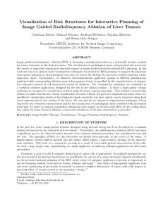
2. PIV visualization utilizing a matched refractive-index method 2.1 Refractive-index adjustment of NaI solution Where the whole three-dimensional flow structure around obstacles is visualized by a PIV technique, it is necessary to match the refractive index of the working fluid with that of the obstacle material. This research employs a sodium iodide solution (NaI solution), which is easy to handle and chemically stable, as the working fluid. This solution is deliberately chosen in order to be able to adjust the refractive index of the working fluid to that of the acrylic obstacle with the index of 1.49. Normally the refractive index of this solution is not so sensitive to temperature change, so that the refractive index of the NaI solution is adjusted by changing its concentration. Figure 1 shows a light path difference caused by refraction, where a YAG laser used in the PIV measurement is irradiated to an acrylic cylinder of 30mm in diameter fixed at a center in a 10cm square acrylic box filled with the NaI solution at 30 degrees Celsius. The light path difference, δ, is measured at a location of 660mm from the back of the cylinder. The difference decreases with the increase in the NaI concentration and reaches zero at 61.6wt%. That means that the refractive index of the NaI solution completely corresponds with that of the acrylic cylinder at this concentration. In actual visualization
www.intechopen.com
4
Aeronautics and Astronautics
experiments, a refractive index at this concentration under visible light, which is 1.485, was always checked by using a portable refractometer before each experiment, because the change in the refractive index might be caused by deposition of NaI crystals onto the pipe wall and/or volatilization from the solution.
Fig. 1. Matched refractive-index experiment using NaI 2.2 PIV measurement with fluorescence particles The PIV utilized in this experiment is a double-pulse YAG laser system manufactured by Japan Laser Corporation. The laser output is 25mJ@532nm and the maximum oscillatory frequency is 30Hz. In the PIV measurement, a time series of tracer particles’ images in a sheet laser is taken with a high speed camera, and, then, a two-dimensional flow structure is quantitatively visualized from the movement of the tracer particles. The time interval of the double pulse and the tracer concentration are adjusted depending on the flow conditions. To process the obtained particle images, a cross-correlation scheme is adopted to get spatially dense velocity information. Furthermore, melamine fluorescence resin particles with 1~20 m diameter are utilized as the tracer particles. The specific gravity of NaI solution at the above mentioned concentration is relatively close to that of this tracer, so that buoyancy influence can be ignored. When this fluorescence particle is irradiated with the YAG laser, it causes excitation in the fluorescent agent which emits light of 580nm wavelength. By taking only this newly emitted light into a CCD camera with an attached filter lens, it makes it possible to obtain a clearer particle image than the usual tracer image, because the diffused reflection light of the laser observed on the pipe wall surface and on the acrylic sphere surface can be completely removed simultaneously.
3. Experimental apparatus and details of test section Figure 2 shows a diagram of the apparatus for the visualization experiment under isothermal conditions. The apparatus consists of the following components: a circulating pump, a flow rate measuring section, a flow-straightened section, a test section, a bag filter, and a mixing tank. All piping materials and components have been made of polyvinyl chloride or acrylic materials etc. which co-exist in a stable state with the NaI solution. The magnetic pump circulates the working fluid inside the loop, and its maximum flow rate under obstacleunpacked conditions is approximately 200l/min. The flow rate of the working fluid is adjusted
www.intechopen.com
Visualization of Complex Flow Structures by Matched Refractive-Index PIV Method
5
by valves: two valves located between the magnetic pump and the flow rate measuring section and a valve of a bypass line which directly returns to the mixing tank from the magnetic pump. A turbine flowmeter or an ultrasonic Doppler velocimeter is utilized to measure the flow rate. The mixing tank has the following functions: injection of tracer particles, de-aeration of bubbles existing in the fluid, and heat exchange to control the fluid temperature. The section upstream of the test section has a flow-straightener with a honeycomb structure consisting of stainless steel pipes, which straightens and counteracts a swirling flow formed in the bend upstream. The bug filter is a polypropylene-made cartridge with strong corrosion resistance which separates the tracer particles from the NaI solution. T
Mixing Tank
Filter P F1 Magnetic Pump YAG Laser
F1 Turbine FlowMeter F2 Ultrasound Dopplere Flow Velocimeter
F2
P
PIV System
P Bourdon Tube Pressure Gauge T Thermometer
CCD Camera
Fig. 2. Experimental apparatus for visualization Figure 3 shows a detailed view of the visualization test section. Here, we focus here on the flow field in a Sphere-Packed Pipe (hereafter, SPP) that is utilized as a heat exchanger and/or a cooling device in various fields (e.g. Yuki et al. 2007, 2008). The test section is an acrylic vertical riser-pipe with D=56mm as inner diameter and 670mm in length. The visualizing area is located at 8.2D (=460mm) downstream from an inlet of the test section where a fully-developed flow is anticipated. In addition, there is a rectangular jacket surrounding the test section in order to reduce image distortion resulting from the geometry of the circular pipe. The NaI solution at the same temperature as the working fluid is also filled into the jacket. In order to visualize the flow field in the lateral cross section of the circular pipe, an acrylic observation window is attached to the upper part of the test section. Figure 2 also shows the packing structure of the acrylic spheres. The sphere size prepared for this research is D/2.0 (27.6mm) in diameter, and 68 spheres can be packed in the test section with a porosity of 0.548. An acrylic baffle plate set between the flanges, which exist at the inlet and outlet of the test section, fixes the acrylic spheres. The temperature of the NaI solution is 30 degrees Celsius, and the visualization of the flow field is conducted at three Reynolds numbers (Red=Ud/ ) of 800, 2000 and 4900, based on the sphere diameter, d, and mean inlet-velocity U. The mean inlet-velocity, which is equivalent to superficial velocity in the SPP, is 0.0376, 0.0940 and 0.230 m/s, respectively. Fand et al. (1990, 1993a, 1993b) have classified the SPP pipe flow with D/d>1.4 into: turbulent regime (Red>120), Forchheimer regime (5