Visualization of Content Information in Networks

Visualization of Content Information in Networks using GlyphNet Anne Denton and Paul Juell Department of Computer Science, North Dakota State University, Fargo, ND 58105 {anne.denton, paul.juell}@ndsu.nodak.edu Abstract. Visualization of information on a graph has two aspects that are equally important in many settings: Visualization of graph connectivity and visualization of node information. We introduce GlyphNet, a tool that displays node-related information graphically, using small icons or glyphs. Our goal is to assist researchers who are applying data mining techniques to relational data, and have a need to identify patterns that involve node attribute values of interconnected nodes. GlyphNet represents node data as glyphs, analogously to the symbols on a weather map. Rather than placing glyphs in a spatial context, as is the case for weather symbols, GlyphNet displays node information in its graph context. We demonstrate the use of GlyphNet for the example of a data mining task that involves yeast gene and protein properties within the corresponding protein-protein interaction network.

1. Introduction Information visualization on a graph is important for many subject areas. Social networks, the link structure of the World Wide Web, and biological networks, such as protein-protein interaction graphs and biochemical pathways, are examples of data that are commonly represented as graphs. Many techniques exist to display such graphs [1]. Most of them do, however, focus on connectivity. Node data, if displayed at all, is usually included in textual form, such as in the class diagrams and entity-relationship diagrams that are common in software engineering. Modern information visualization tools add several aspects to traditional graph drawing. Graph navigation allows a user to view detailed information around a node of interest while, at the same time, allowing access to the rest of the graph. It is common that computer-based tools also provide probe functionality to display node details in a separate window, based on selections made by the user. A good example of probe functionality is implemented in the Web navigation tool TouchGraph WikiBrowser [2] that allows navigation within the link structure of Web pages while making the content of individual pages available separately. The user has the option of selecting a page through mouse click that will then be displayed in a separate browser window. Although this is an efficient solution to the problem of retrieving information from a network of nodes, it is not suitable to typical data mining tasks such as the identification of interesting patterns. Visual data mining can be seen as a hypothesis generation process [3]. We will, therefore, now look at possible hypotheses that can be generated from different graph visualization tools. Traditional graph drawing techniques that display nothing but connectivity allow investigating hypotheses on the distribution of edges. Many interesting results can come from such studies, e.g., the identification of different types of networks [4], including scale-free networks and random networks. Graph visualization tools with probe functionality allow generating hypotheses that go beyond connectivity alone. A particular node can be viewed within the nodes in its network neighborhood, which can, for example, allow generating hypothesis regarding relationships between edge distribution and node importance. Google’s PageRank [5] algorithm that relates the importance of a Web page to the distribution of incoming links would be accessible to such analysis. Much work is still being done to improve on importance measures [6], and a graph visualization tool with probe functionality could be used productively in this context. Much current work in the area of data mining involving relational data does, however, go beyond the issues addressed so far [7]. The term relational data refers to data in which a relationship exists between data records that can be represented by a graph. Typical questions of interest are how relational neighbors can or should be used in classification and clustering [8]. Such questions require access to node data of not only one node but of all nodes for which a hypothesis is to be made. In very small graphs one may try to resolve the problem by including a textual representation of the node data into the graph, as is done in class diagrams and entity relationship diagrams. When this strategy is used many problems of textual representations recur that were supposed to be addressed by the visualization: Textual information has to be interpreted and patterns are, therefore, hard to see. Text also uses up a significant amount of space, which limits the number of nodes that can be displayed simultaneously.

In this paper we introduce a tool to visualize node data through glyphs, small graphical representations of the node attribute values. We thereby provide a valuable tool for the visual exploration of data that is characterized by graph connectivity as well as node data. Our tool is intended to generate hypotheses that involve attributes in multiple, connected nodes. Hypotheses may then be validated through numerical techniques. Why couldn’t one find all interesting patterns numerically? For relational data the search space for interesting patterns is very large. Not only is it possible that attributes within one record affect each other, rather all the attributes of a neighbor, a neighbor’s neighbor etc. can affect the properties of a given node. Although it may be hard to specify how an interesting pattern should look like, a human may still be able to detect it. There is, furthermore, still a lack of data mining techniques that are suitable to the relational setting, although some progress has been made recently [7]. Many traditional data mining techniques exist that were developed for data in a simple tabular form. Making use of the richness and sophistication of these techniques in a relational setting is possible if the characteristics of the data can be handled through preprocessing techniques, in particular, feature extraction. Feature extraction refers to the process of identifying relevant patterns that can then be included into a tabular format. A relevant feature in the relational setting could be the number of neighbors of a node for which a particular Boolean property is “true”. Section 5 will discuss an example use of GlyphNet in which this type of feature extraction is used in conjunction with a classification algorithm [9]. The paper is organized as follows: Section 2 provides details on existing graph visualization techniques. Section 3 discusses the concepts and common uses of glyphs for the visualization of attribute values in a large number of data records. Section 4 introduces GlyphNet and explains how the concepts of graph visualization and attribute representation through glyphs are implemented in this tool. Section 5 gives an example of how GlyphNet can be used as a visual data mining tool for the purpose of identifying candidates for feature extraction in a classification task. Section 6 concludes the paper.

2. Graph Visualization Techniques We will now discuss in some more detail how existing techniques are related to ours. Graph drawing is an old topic and many techniques exist for its purpose [10]. One main goal in traditional graph drawing, planarity, consists in avoiding crossing edges. Other aesthetic rules have been formulated, including the goal that edges should be represented by straight lines, all edges should have the same length, and isomorphic structures should be displayed equivalently. These goals are easier to achieve for tree layouts than for general graphs. A common technique for a general graph, therefore, consists in finding a spanning tree and calculating the layout for the spanning tree. Additional edges are added later, and edge crossings are ignored for those additional edges. Many layouts have been described in the literature, including top-down layouts like the Reingold and Tilford layout [11], the H-tree layout [12], a layout with radial positioned nodes [13], and the balloon tree layout [14]. These traditional tree designs are deterministic, i.e. the same tree is always laid out in the same way, independently of the initial state of the program that is used to draw it. The layout used in GlyphNet is based on a Force-Directed Method [15], in which nodes are modeled as physical bodies with the edges representing springs that hold them together. The corresponding mathematical optimization problem is known to produce well-balanced graphs with a small number of edge crossings [16]. In contrast to traditional tree layouts, this layout technique is not deterministic. Time complexity of force-directed algorithms makes them mainly suitable to small graphs, which is acceptable in a graph navigation system that only displays a small part of the graph at any one time. Many current problems involve graphs that are too large to display in such a way that all nodes can simultaneously be viewed with sufficient detail. Traditional techniques are therefore often combined with graph navigation features that allow displaying only those nodes that are within a predefined distance of a central node. Alternatively the plane may be distorted using either hyperbolic geometry [17] or a fisheye view [18] to provide detail in the vicinity of a selected node. More distant nodes are displayed with less detail and serve the purpose of providing a context. In either case, navigation is achieved by letting the user select a central node, and calculating a new layout for each new choice. GlyphNet uses the former strategy of displaying a limited number of nodes. This avoids confusion that could come from distorting glyph information. Adding node information to graph layouts can be done in several ways. A common strategy consists in representing nodes through text boxes as in class diagrams and entity relationship diagrams. In

this paper we will focus on techniques that add node information in graphical form, since they are most closely related to GlyphNet. Some existing approaches represent one or two items of information in graphical form using node size and/or node color. These approaches commonly use textual information as well as possibly probe capability to represent the majority of node content. An example of a visualization that uses node size to represent one item of information in graphical form is the SGI File System Navigator [1]. This tool displays a virtual landscape representation of a computer file system. The file structure itself is displayed as a two-dimensional landscape that can be explored by a “fly through” of a three-dimensional world above the surface. File size is represented as the size of buildings in the virtual landscape. An example of a visualization that can use node color for the representation of node information is a cone tree [19]. A cone tree is a visualization of a tree within three dimensions. Child nodes are placed along the base of a cone that represents parent information. Color can be used besides text to display node content. Newer versions of the algorithm use cone size as well as color for the representation of node information [20]. The cone tree concept cannot be used for graphs in general since it relies on the hierarchical organization of the data. Another example of a visualization that can use both color and size to represent up to two items of information per node is a tree map [21]. In this design, leaf nodes of a tree are laid out as rectangles in a plane. Internal nodes are identified either through choice of a common color for lower level nodes or through boundaries surrounding lower level nodes. In the latter case color may be used to represent node information as well as size of the rectangles. In a practical application of a tree map, a map visualizing stock performance [22], color represents performance of stock, and size represents volume. The tool furthermore provides probe information in response to mouse movement and clicks. The tree map design is limited to hierarchical data and cannot be generalized to other graphs because edges are not explicitly represented. This is the maximum number of graphically represented attribute values the authors have found for any existing graph visualization. In section 3 we will introduce glyphs as a way of representing multiple items of information. A concept that is related to glyphs is used in graph clustering [23]. Complex graph structures can be made accessible by grouping related nodes into clusters. These clusters may then be represented in a summarized fashion at a higher level. The process may be iterated to result in a hierarchical structure of graph clusterings. [23] uses a polygon to represent each lower level cluster at a higher level. The shape of polygon is chosen such that it matches the shape of the lower-level cluster by some criteria. This use of glyphs differs from ours in its goal of representing connectivity information only. Representing connectivity information in a summarized fashion can assist in understanding the structural properties of a graph but does not solve the problem of representing independent node information.

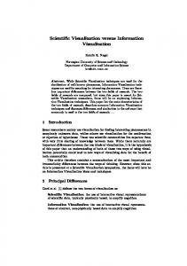
3. Visualization of Attributes Using Glyphs A glyph is a graphical object used to display one or more dimensions of information [24]. Each glyph represents one record of data. Many or all records can be displayed simultaneously. Interesting properties of the data can then be identified as graphical patterns within the glyph without a need to refer to the actual data. Relationships between different records can be identified through comparison of different glyphs. Glyph representations vary in the way they represent attributes graphically, and also in the way the individual glyphs are organized with respect to each other. Glyphs are designed to have several parts that can be modified individually. Each part is used to display an attribute or dimension of the information. Well known types of multidimensional glyphs are cartoon faces that use one variable to select the eyes, another to select the nose and so on [25]. These are commonly known as Chernoff faces. A motivation for using Chernoff faces is that human viewers are particularly familiar with facial features. Frequent attribute combinations can thereby be identified as a particular kind of face. Another well-known data representation is a star glyph [26]. Star glyphs arrange attributes in a circular fashion with scales for each variable extending from a center outward. Points on neighboring scales are connected. This produces a closed pattern that allows seeing proportional relationships between variables [27]. See Figure 1, left side, for an example of a star glyph. It is important for the usefulness of this design to place attributes in such a way that within most records attributes with a large value tend to be neighbors of attributes with a small value. This results in a particularly star-like shape. Based on guidance from Tufte [28] the display should be as simple and clean as possible, so we do not show the scaling marks or other items, just the data values.

So far we have discussed differences between glyph patterns but have not yet looked at differences in how glyphs may be arranged. In some but not all cases the arrangement of glyphs on the plane may come naturally. Weather maps represent weather information that has been collected from particular spatial locations, and weather glyphs are therefore represented within spatial dimensions. Sometimes the information collection may inherently one-dimensional, such when drilling for raw materials [26]. Finally there may be no “natural” dimensions for the organization of glyphs at all. In that case placement can be chosen to be convenient for the data mining process, such as ordering by attributes of the represented records. In our case the glyph placement is determined by the graph layout, leading to additional challenges. Glyphs information of neighboring nodes should not be confused, and lines that represent edges should not interfere with the glyphs themselves. Spatially organized data such as weather data, in contrast, is commonly collected at locations that are sufficiently separate to eliminate such problems. In graph layout algorithms separation of nodes and equal length of edges are goals but may not be satisfied perfectly. We choose to embed each glyph in a circle that clearly identifies the node. The area within the circle is reserved for the node, and edges are hidden behind it. We found that this concept works well, provided the design of the glyph is adapted to the new setting. It can be seen in Figure 1 (left) that a star glyph does not fill the circle well, and much space is wasted. We therefore designed a glyph shape such that it fills the circle fully if all attributes have their maximum value. The circle is divided evenly into wedges or pie-slices, one for each attribute, with the radius representing the attribute value Figure 1 (right). It should be noted that the area of a wedge increases as the square of the radius. We did not use glyphs for quantitative analysis and chose the scaling of attributes entirely based on how clearly values could be distinguished. For quantitative analysis it would be necessary to take a decision on whether radius or area should be used as a measure of the attribute value and the scaling would have to be chosen accordingly.

Fig. 1. Comparison between star (left) and wedge glyph (right) The glyph design offers other degrees of freedom, in particular color, which can be included in the visualization process. For the current purpose the overall color was chosen as the only relevant item of information. Section 4 will discuss the use of color in more detail.

4. Description of GlyphNet The design of GlyphNet is based on public domain software, Touchgraph [29], which is available from the SourceForge open source software development web site. The goal of the Touchgraph project is to provide a user interface for the exploration of web pages. The graph layout algorithm used in the project is based on a force-directed layout [15], and large graphs are made accessible through navigation [1]. Nodes that exceed a predefined number of edges from a selected central node are hidden. A new central node is selected through mouse click. The subset of nodes that are displayed is automatically adjusted. The maximum distance from the central node can be selected by the user. It is furthermore possible to move a node around by dragging the mouse. The remaining nodes follow according to the force laws that determine the layout. Several versions of the software exist, featuring different aspects of the graph exploration task. Most versions use textual information to identify nodes. Colors are used to distinguish nodes that have a special role in the navigation algorithm, such as the central node and the node or edge that the mouse currently points to. This is particularly important for implementations that use probe functionality, i.e.,

display web page content of the currently selected node in a separate window. An example of such an implementation is the WikiBrowser [30]. Additional labels are attached to nodes for which neighboring nodes are omitted because of their distance to the central node. These labels show the number of omitted nodes and have yet another color in the original implementation. This gives an indication as to the intention of color use in previous implementations. Following the goal of simplifying navigation in a network of web pages, color has been exclusively used to simplify navigational tasks and summarizing structural properties of hidden parts of the graph. We will see later how the use of colors for navigational purposes had to be limited in GlyphNet so as to minimize confusion with data mining goals. GlyphNet represents node information in graphical form for all nodes within the displayed range. Figure 2 shows a snapshot of GlyphNet for a graph that represents protein-protein interactions in yeast. Node data includes properties of yeast genes and of their corresponding proteins. Details of the underlying biological system will be given in Section 5. In the example in Figure 2 the maximum distance of nodes from the central node is two. Nodes that are further away than two edges are hidden but may be exposed by selecting a different central node or increasing the range of displayed nodes. GlyphNet was derived from other graph visualization tools by replacing node identifiers with glyphs that visualize node attributes through shape and color. Displaying node identifiers as well as glyphs for all nodes was considered too confusing. Node identifiers are, however, displayed when the mouse is placed over a node, following the probe concept. For the current implementation, the probe mechanism is limited to the display of node identifiers, but an extension to a more extensive textual display of node content would be straight-forward.

Fig. 2. Snapshot of GlyphNet for yeast gene and protein data within the graph of protein-protein interactions. We had to reduce the use of color for navigational purposes in order to limit confusion with color choices that represent node data. We chose to use the same, blue, color for all structural information that is static, including the labels that summarize the number of hidden neighbors, such as, for example, the number 1 in the top right corner of the lower red node. If that red node is selected as central node it shows an additional edge that is currently hidden, as well as neighbors to the newly exposed node. Color changes that are related to mouse movement were kept since the user can easily get an undisturbed image by moving the mouse off the graph display area. In particular, the highlighting of the node to which the mouse currently points was kept. Notice the gray background of the node that is identified through the node label

“YBR155W”. Maintaining this aspect of the navigation-related color information was possible due to the fact that the color that fills the circle is redundant in our color scheme if the color of wedges is known. Section 5 gives details on the node and interaction data in this particular example. Six attributes are encoded in each node. One attribute of special interest determines the color, with the three color choices being green, red and yellow. Five other attributes determine the size of the pie slices. The background color within each node is chosen as a brighter version of the pie slice color. More color information could be used but didn’ t lend itself to the particular data mining task described in section 5. The edges don’ t contain directional information since the yeast interaction data is undirected. Directional information can easily be included through use of wedges for links. This representation is implemented in the TouchGraph web visualizations [29] that have to distinguish between incoming and outgoing links to web pages.

5. Example Use of GlyphNet for Yeast Data Visualizations are as good as the insights they can give. For the purpose of visual data mining we are interested in hypotheses regarding patterns within the data. We used GlyphNet as part of a data mining task in bioinformatics. The goal was the identification of yeast genes that were involved in a particular pathway, the Aryl Hydrocarbon Receptor (AHR) pathway. In data mining terms this is considered a classification task: Genes that are part of the AHR pathway were classified as “change”, genes that were not part of the pathway, or for which no experiment had been performed, as “no change”, and genes that responded to a control experiment as well as to the AHR-related experiment were “control” [30]. The classes were determined in a high-throughput gene deletion experiment. 5000 strains of yeast, each of which was the result of the deletion of a specific gene, were simultaneously treated in micro-array experiment. The overwhelming majority, 97%, of genes belonged to the “no change” class. In Figure 2 “change” genes are identified by their red color and “no change” genes by their green color. Yellow was picked as color for “control” genes and can be seen in Figure 5. Figure 3 provides a summary of the information that was encoded in each node. The pie slice at the top indicates whether a gene is essential. If a gene is essential the organism will die if that gene is deleted. Gene deletion experiments can therefore not be used to gain information for essential genes. The property “essential” is Boolean, i.e., the pie slice is either filled fully or not at all. The same applies to the “pseudo gene” property in the lower left of the glyph. A pseudo gene is a gene that is known not to produce a functioning protein. All other properties are numerical. The distance of a gene from the center of the chromosome (top right) was estimated as follows: Genes are numbered sequentially, starting from the center of the gene, and this number is part of their name, i.e., the gene “YBR155W” in Figure 2 has the number 155, which is taken as distance from the center of the chromosome. The number of amino acids of a gene was taken as its length (top left). Finally we counted the items of information that are given for the protein that a gene produces. Items of information were functions, localizations, and some other quantities that were provided for the KDD cup 2002 [31] and are also available from the Comprehensive Yeast Genome Database at the Munich Information Center for Protein Sequences, MIPS [32].

Fig. 3. Meaning of attributes for the glyphs used in Figure 2.

but not

Fig. 4. Left: example of a pattern we identified; right: typical pattern that standard algorithms could find but that cannot be present in the current data. For the evaluation of our visualization tool we will focus on the property “ essential” that is displayed at the top of the glyph since it leads to the clearest hypothesis with respect to the AHR pathway property. Looking at Figure 2 it can be seen that the red, “ change” gene at the center has two out of four neighbors with the property essential. The “ change” gene in the bottom right only has a single neighbor which also has property “ essential” . Over the entire range of nodes only four out of a total of 22 “ no change” genes have the property “ essential” . Note that “ change” genes cannot be “ essential” since the deletion experiment cannot be performed on “ essential” genes. Figure 4 highlights the unusual aspect of our hypothesis. The navigation capability of GlyphNet allows us to systematically follow patterns that could be interesting. After identifying the potential pattern of an “ essential” gene that interacts with a “ change” gene we may want to investigate the neighborhood of further “ essential” and “ change” genes to support our observation. Figure 2 shows one “ essential” gene in the top half. Although that gene does not have hidden neighbors we may want to investigate its further neighborhood and therefore make it the central node. Figure 5 shows the result of that selection. It can be seen that at a distance of two hops (next nearest neighbor) there is a “ control” gene (yellow) that has also an “ essential” neighbor. This suggests that “ essential” may be an indication of either “ change” or “ control” .

Fig. 5. Snapshot suggesting an impact of “ essential” in a neighbor on the prediction of a “ control” gene.

It is important to note that such hypotheses do not have to mean anything by themselves since we are only investigating a small part of the full graph of several thousand genes. Visual exploration should be considered a part of a more extensive data mining strategy that includes verification of hypotheses through quantitative numerical methods. A classification algorithm was used for this purpose as described in [9]. The pattern in Figure 4 entered the classification algorithm in the shape of an additional attribute that represented the number of interacting “ essential” genes. A genetic algorithm was used to determine attribute importance, and “ essential” /” change” pattern was shown to improve classification significantly. The validity of the visual exploration results was thus verified. Improvement of classification results is particularly clear when “ change” and “ control” are considered together as one class and “ no change” as the other class, supporting the visual exploration result that “ essential” is an indication for both “ change” and “ control” in a neighbor. This shows the potential of employing GlyphNet in a visual exploration process as part of a comprehensive data mining strategy. Given the prevalence of relational data in current data mining tasks and the difficulty of handling it with current data mining techniques, GlyphNet is an important tool to provide leads on interesting patterns.

6. Conclusions We have introduced a tool, GlyphNet, that assists in the data mining of relational data by combining the concept of glyphs with graph visualization and navigation. Relational data provides particular challenges to the data mining process due to the complexity of potential patterns. Patterns in relational data can involve attributes of multiple interconnected nodes, making traditional data mining and visualization techniques hard to apply. Our tool is designed specifically to assist in the discovery of such patterns. An example of a data mining task for genomics data was presented. We demonstrated how a hypothesis involving attributes of neighboring nodes was generated through GlyphNet. The usefulness of the hypothesis was verified by a quantitative data mining algorithm. We have therefore demonstrated the potential of GlyphNet to assist in a data mining process involving relational data. Many further applications can be envisioned since pattern discovery is a central part of most areas of data mining.

References 1. 2. 3. 4. 5. 6. 7. 8. 9.

I. Herman, G. Melancon, and M. S. Marshall, “ Graph Visualization and Navigation in Information Visualization: A survey,” IEEE Transactions on Visualization and Computer Graphics, Vol. 6 No. 1, pp. 24-43, 2000. http://touchgraph.sourceforge.net/ Daniel A. Keim: Information Visualization and Visual Data Mining. IEEE Transactions on Visualization and Computer Graphics, Vol. 8, No. 1, pp. 1-8, 2002. A. L. Barabasi and E. Bonabeau, “ Scale-free networks,” Scientific American, Vol. 288, No. 5., pp.6069, 2003. L. Page, S. Brin, R. Motwani, T. Winograd, "The PageRank citation ranking: Bringing order to the Web," Stanford Digital Libraries Working Paper, 1998. S. White and P. Smyth, “ Algorithms for Discovering Relative Authority in Graphs,” The Ninth ACM SIGKDD International Conference on Knowledge Discovery and Data Mining (KDD-2003), Washington, DC, 2003. L. Getoor, N. Friedman, D. Koller, and A. Pfeffer, “ Learning Probabilistic Relational Models,” Relational Data Mining, S. Dzeroski and N. Lavrac, Eds., Springer-Verlag, 2001. S. A. Macskassy and F. Provost, “ A Simple Relational Classifier,” Workshop on Multi-Relational Data Mining in conjunction with KDD-2003 (MRDM-2003), Washington, DC, 2003 Amal Perera, Anne Denton, Pratap Kotala, William Jockheck,Willy Valdivia Granda, and William Perrizo "P-tree Classification of Yeast Gene Deletion Data." SIGKDD Explorations, Vol. 4, Issue 2, pp. 108-109, January 2003.

10. G. di Battista, P. Eades, R. Tamassia, and I.G. Tollis, “ Graph Drawing: Algorithms for the Visualization of Graphs,” Prentice Hall, 1999. 11. E.M. Reingold and J.S. Tildford, “ Tidier Drawing of Trees,” IEEE Transactions on Software Engineering,” Vol. SE-7, No. 2, pp. 223-228, 1981. 12. Y. Shiloach, “ Arrangements of Planar Graphs on the Planar Lattices,” PhD Thesis, Weizmann Institute of Science, Rehovot, Israel, 1976. 13. P. Eades, "Drawing Free Trees," Bulletin of the Institute for Combinatorics and its Applications, pp. 10-36, 1992. 14. J. Carrière and R. Kazman, "Research Report: Interacting with Huge Hierarchies: Beyond Cone Trees," Proceedings of the IEEE Conference on Information Visualization ‘95, IEEE CS Press, pp. 7481, 1995. 15. P. Eades, “ A Heuristic for Graph Drawing,” Congressus Numeratium, Vol. 42, pp. 149-160, 1984. 16. A. Frick, A. Ludwig and H. Mehldau "A Fast Adaptive Layout Algorithm for Undirected Graphs," Proceedings of the Symposium on Graph Drawing GD ' 93, Springer Verlag, pp. 389-403, 1994. 17. J. Lamping, R. Rao, and P. Pirolli, "A Focus+context Technique Based on Hyperbolic Geometry for Visualizing Large Hierarchies," Human Factors in Computing Systems, CHI ’ 95 Conference Proceedings, ACM Press, 1995. 18. M. Sarkar and M.H. Brown, "Graphical Fish-eye views of graphs," Human Factors in Computing Systems, CHI ’ 92 Conference Proceedings, ACM Press, pp. 83-91, 1992. 19. G.G. Robertson, J.D. Mackinlay, and S.K. Card, "Cone Trees: Animated 3D Visualizations of Hierarchical Information," Human Factors in Computing Systems, CHI ’ 91 Conference Proceedings, ACM Press, pp. 189-194, 1991. 20. M. Hemmje, C. Kunkel, and A. Willet: "LyberWorld - A Visualization User Interface Supporting Fulltext Retrieval," Proceedings of ACM SIGIR’ 94, ACM Press, 1994. 21. B. Johnson and B. Schneiderman, "Tree-maps: a Space-filling Approach to the Visualization of Hierarchical Information Structures," Proceedings of IEEE Visualisation’ 91, IEEE CS Press, pp. 275282, 1991. 22. http://smartmoney.com/marketmap/ 23. P. Eades, Q. Feng, “ Multilevel Visualization of Clustered Graphs,” Lecture Notes in Computer Science” , 1190, pp 101-112, 1997. 24. Hearn, Donald and M. Pauline Baker, Computer Graphics: C Version, Prentice Hall, 1997. 25. Chernoff, H., Using Faces to Represent Points in K-Dimensional Space Graphically, J. American Statistical Association, Vol. 68, pp. 361-368, June 1973. 26. D. Hand, H. Mannila, and P. Smyth, “ Principles of Data Mining” , The MIT Press, Cambridge, MA, 2001, p. 75. 27. G. E. Jones, “ How to Lie with Charts,” Authors choice Press, Lincoln, NE, 2000. 28. Tufte, E. R., The visual display of quantitative information, Graphics Press, Cheshire, CT, 1990. 29. http://touchgraph.sourceforge.net/ 30. http://prdownloads.sourceforge.net/touchgraph/TGWB_102.zip 31. M. Craven, “ The genomics of a signaling pathway: a KDD Cup challenge task SIGKDD Explorations,” Vol. 4, Issue 2, pp. 97-98, January 2003. 32. http://mips.gsf.de/genre/proj/yeast/index.jsp