Visualization of Diffusion Propagator and Multiple Parameter Diffusion Signal Olivier Vaillancourt and Maxime Chamberland and Jean-Christophe Houde and Maxime Descoteaux1
Abstract New advances in MRI technology allow the acquisition of high resolution diffusion-weighted datasets for multiple parameters such as multiple q-values, multiple b-values, multiple orientations and multiple diffusion times. These new and demanding acquisitions go beyond classical diffusion tensor imaging (DTI) and single b-value high angular resolution diffusion imaging (HARDI) acquisitions. Recent studies show that such multiple parameter diffusion can be used to infer axonal diameter distribution and other biophysical features of the white matter, otherwise not possible. Hence, this calls for novel visualization techniques to interact with such complex high-dimensional and high-resolution datasets. To date, there are no existing visualization techniques to visualize full brain images or fields of diffusion signal profiles and diffusion propagators reconstructed from them. It is important to be able to scroll in these images beyond single voxels, just as one would navigate in a whole brain map of fractional anisotropy extracted from DTI. In this chapter, we give a review of the existing visualization techniques for the local diffusion phenomenon and propose alternative visualization techniques for fields of highdimensional 3D diffusion profiles. We introduce: i) a volume rendering approach and ii) a diffusion propagator silhouette glyph as a complement to existing DTI and HARDI visualization techniques. We show that these visualization techniques allow the real-time exploration of high-dimensional multi-b-value and multi-direction data such as diffusion spectrum imaging (DSI). Our visualization technique therefore opens new perspectives for 3D diffusion MRI visualization and interaction.
Sherbrooke Connectivity Imaging Lab (SCIL), Computer Science department, Sherbrooke Molecular Imaging Center (CIMS), Universit´e de Sherbrooke. 1 e-mail:
[email protected]
1
2
Vaillancourt et al.
1 Introduction New advances in multi-band acquisition [1, 2, 3], in compressed sensing technology [4, 1], improvements in magnetic resonance (MR) hardware [3, 1], such as multi-channel head coil allowing fast parallel imaging , and novel diffusion imaging sequences allow the acquisition of many diffusion measurements in reasonable time. The motivation for these demanding acquisitions is to obtain both the radial and angular part of the diffusion signal at potentially multiple diffusion times. Hence, going beyond classical diffusion tensor imaging (DTI) and high angular resolution diffusion imaging (HARDI) tractography applications. In fact, not only is it nowadays important to densely measure the radial and angular part, but it is important to do so at multiple echo times (TE) [5, 6, 7]. Recent studies show promising multiparameter diffusion techniques for axonal diameter distribution estimation and to study demyalination and abnormal white-matter tissue [8, 6, 9]. To date, there are no available visualization techniques to efficiently visualize a 2D field or full brain of such 3D diffusion images and diffusion propagators. The diffusion propagator is the full 3D probability distribution function describing the probability that a water molecule starting at origin will have displaced to a certain location during the diffusion time. Visualization of these 3D diffusion profiles is crucial to explore, analyze and understand the data efficiently in order reinforce hypothesis building and understanding of the data acquisitions, noise and features present in the data. In this chapter, we first revisit the theory of the 1D and 3D q-space imaging and give a brief overview of existing visualization techniques. We then introduce two alternative ways to visualize fields of 3D diffusion profiles. We propose i) to use a direct volume rendering method and ii) define a new diffusion propagator silhouette glyph. We show that these visualization techniques allow the real-time interaction with complex 3D diffusion datasets and open new perspectives in diffusion MRI exploration. All software solutions are open and publicly available to the community.
2 Theory 2.1 Diffusion-weighted imaging and Q-space Imaging It is well-known that the diffusion-weighted signal is tuned with two key parameters: the direction of the applied diffusion gradients and a b-value acting like an inverse zoom factor, e.g. the higher the b-value, the smaller the range of the displacement of molecules observed. While these parameters are still used in clinical applications, they are inadequate to describe the basis of possible displacements in porous media. In 1991, Callaghan introduced q, representing the wave vector of displacements and leading to the dual space of displacement vectors, called qGγ . The q wave vector is linked to the width (δ ), the magnitude space [10, 11]: q = δ2π
Diffusion Propagator Visualization
3
(|G|) and orientation of the diffusion gradient pulse (G) of the diffusion sequence. The b-value itself is linked to the square of the q vector and the diffusion time τ: b = 4π 2 q2 τ and τ = (∆ − δ3 ), where ∆ is the time between the two diffusion gradient pulses. The diffusion time thus corresponds to the duration of the observation of the diffusion process. This parameter is generally untuned but is the result of the optimization of the TE under the constraint of the chosen b-value, the hardware characteristics (maximum amplitude and slew-rate of the gradients and safety considerations). Yet, in recent AxCaliber and ActiveAx techniques [7, 9], diffusion acquisitions are done for multiple b-values, multiple gradient orientations as well as multiple TEs to be sensitive to different underlying microstructural sizes. A very powerful illustration of the potential of these equations is Fig. 1. We see the evolution of the diffusion-weighted signal attenuation according to the magnitude of the q wave vector in a simple media composed of a network of impermeable cylinders filled with water. The attenuation is measured in the direction perpendicular to the axis of the cylinders and shows a typical diffraction phenomenon occurring because of water molecules hitting the boundaries of the cylinders. This simple 1D q-space imaging experiment illustrates how diffusion imaging could be used to probe microstructure of porous media and infer information about its compartments, shape and size. One-dimensional q-space imaging was then generalized to 3D q-space imaging. Under the narrow pulse approximation [13], the relationship between the diffusion signal, E(q), in q-space and the ensemble average diffusion propagator , P(R), in real space, is given by a Fourier transform (FT) relationship [11] such that
Fig. 1 Figure adapted from Kuchel et al [12] representing the 1D q-space imaging diffusion signal attenuation decay curves for water in suspensions of human erythrocytes as a function of q-value at different hematocrit. The different curves on the graph represent the hematocrit values in decreasing order from the top of the figure, starting from a value of 93%, followed by 83, 73, 63, 47, 42, and 25% at the bottom of the figure. The shaded area represents the range of q values that are currently achievable on clinical MRI systems.
4
Vaillancourt et al.
Fig. 2 Single voxel illustration of the Fourier relationship between measured 3D q-space diffusion signal (left) and 3D diffusion propagator or displacement probability (right).
Z
P(R) =
q∈ℜ3
E(q)e−2πiq·R dq,
(1)
where E(q) = S(q)/S0 , S(q) is the diffusion signal measured at position q in q-space related to the b-value and S0 is the image without diffusion. We denote q = |q| and q = qu, R = rr, where u and r are 3D unit vectors. Eq. 1 suggests a way to reconstruct the diffusion propagator; acquiring as many diffusion images E(q), along as many q-vectors q as possible, before taking a Fourier transform to obtain the diffusion propagator P(R). This is illustrated in Fig. 2 and is at the heart of Diffusion Spectrum Imaging (DSI) [14] , which was recently used in several seminal papers exploring new theories of the grid organization of the brain [15] and connectomics studies [16, 17]. Eq. 1 opens the way to several new acquisition schemes. Fig. 3 highlights the three most used q-space sampling strategies: i) sampling the Cartesian grid, ii) multiple b-value shells in q-space and iii) radial q-space lines. Every sampling scheme leads to a different reconstruction technique of the propagator and adapted mathematical tools for it.
a) Cartesian
b) Spherical
c) Radial
Fig. 3 2D slice representation of different q-space sampling schemes used to measure the diffusion signal and reconstruct the diffusion propagator.
Diffusion Propagator Visualization
5
2.2 Existing visualization techniques for diffusion imaging To the best of our knowledge, there is no technique to visualize a field of diffusion propagators, or 3D diffusion signal profiles arising from DSI [14], multiple b-value diffusion-weighted imaging (DWI), and hybrid diffusion imaging (HYDI) [18]. As seen in Fig. 5, some techniques have been proposed at the voxel level, using i) projections of isocontours along a certain view [14] (Fig. 5a), ii) intersecting orthogonal planes [14] (Fig. 5b), or iii) multiple concentric shells representing isosurfaces of the diffusion propagator [19] (Fig. 5c). It is true that a naive implementation of these techniques would be possible to make them visualize whole fields and volumes of diffusion data. However, making a useful tool to explore high-dimensional diffusion MRI data interactively is essential and non-existant at this time. Multiple-parameter diffusion MRI visualization will become important at the era of multiple b-value and multiple TE diffusion data acquisitions. This chapter sets the table for future visualization research. It is also possible to visualize fields of isosurfaces of a certain radius (Fig. 5b) or fields of orientation distribution function (ODF) computed from the diffusion propagator [14, 20, 18, 21, 19, 22]. The ODF is computed with the equation: Z ∞
Ψ (θ , ϕ) =
P(rr, θ , ϕ)r2 dr,
(2)
r=0
which describes the diffusion ODF in unit direction r = (θ , ϕ), because computed as the radial integral of the diffusion propagator . Many other HARDI angular profiles exist and a very popular one is the fiber ODF reconstructed using spherical deconvolution techniques [23]. High-order tensor glyphs for HARDI also exist [24, 25, 26, 27, 28] to generalize diffusion tensors from DTI and capture the apparent diffusion coefficient, the Kurtosis tensor [29] or a generalized tensor [30] from HARDI data. In all cases, the angular profile is visualized as a spherical function, where the radius of the sphere is scaled according to the spherical function at
Fig. 4 Angular profile visualization with the orientation distribution function (ODF) glyph, Ψ (θ , ϕ). The radius of a spherical mesh is scaled according to the value of the sphere.
6
Vaillancourt et al.
a) Isocontours visualization [14]
b) Isosurface and ODF [20]
c) Multiple concentric shells [19]
Fig. 5 Existing techniques to visualize the diffusion propagator and 3D q-space diffusion profile. All these techniques work only for a single voxel and do not exist to image a full brain or even a field of diffusion propagators. In a), different 2D slices of the 3D diffusion signal profile (1st row) and propagator (2nd row) are seen, as well as an isosurface glyph through the volume. These images are adapted from [14, Fig.2]. In b), the diffusion propagator (also called 3D displacement distribution) is visualized using three orthogonal planes through its center. Below, an isosurface glyph at radius 5 of the propagator and a diffusion ODF integrating the propagator over radii. Images are adapted from [20, Fig.6]. In c), multiple concentric shells are seen on top of one another. Each shell represents an isosurface glyph overlaid with a different opacity and, a colormap from black to red for low to high isosurface radii of the propagator. Images are adapted from [19, Fig.6].
Diffusion Propagator Visualization
7
Fig. 6 Different prolate and oblate diffusion tensors visualized with classical ellipsoids (top) and superquadrics (bottom). Superquadrics are adapted from Kindleman et al [32] and provide better perceptual cues than ellipsoids.
each vertex of the sphere mesh. This is illustrated in Fig. 4, where we see how each vertex point (θ , ϕ) of the spherical mesh is scaled to radius r = Ψ (θ , ϕ). Data visualization for diffusion tensor imaging (DTI) is more developed. In DTI, classic ellipsoidal glyphs are used [31], superquadrics [32, 33], supertoroids [34], tensor glyphs [35] or more complex glyphs [36], highlighting the linear, planar or isotropic parts of the diffusion tensor, as seen in Fig. 6. New DTI glyph developments arise from the need to increase orientation and depth perception for single glyphs, and improve data inter-relation perception for glyph fields. As seen in Fig. 6, advances in DTI glyphs provide perceptual cues that reduce ambiguities caused by precedent models and thus must be considered in the creation of new diffusion glyph models beyond DTI. In this regard, the proposed diffusion propagator silhouette glyphs in this chapter are inspired by [36] and superquadrics from [33] to allow the visualization of fields of propagators or 3D diffusion signal profiles.
3 Methods 3.1 Dataset for visualization A standard DSI acquisition mimicking the original DSI protocol [14] was done on a 3 T system (Philips Achieva X, Best, The Netherlands), equipped with a whole body gradient (40 mT/m and 200 T/m/s) and a 8-channel head coil. Single-shot spin-echo EPI measurements with isotropic 2 mm spatial resolution and 515 diffusion measurements were acquired including q-space points of a cubic lattice within the sphere of five lattice units in radius. TE/TR= 116 ms/14.9 s (including time for dynamic B0 stabilization), bandwidth in EPI direction= 1101 Hz, 128x128 matrix, 60 axial slices with a parallel imaging (SENSE) factor of 2, delta and Delta were
8
Vaillancourt et al.
45.4 and 57.7 ms and maximal b-value of bmax = 6000 s/mm2 . The estimated SNR in the white matter was approximately 38 for the b = 0 image, as computed by dividing the mean signal value in the white matter by the noise standard deviation σ estimated using PIESNO [37]. The PIESNO framework [37] is robust to Rician and non-Central chi distributed noise arising from multiple channel imaging data reconstructed with SENSE or GRAPPA [37]. Fig. 7 shows an axial slice with background voxels automatically detected by PIESNO and then used to infer the noise standard deviations σ from these voxels. Note that the PIESNO technique is not met to do a precise brain extraction or skull strip, but used to identify voxels that all have the same underlying noise statistics. Hence, it is expected that the background voxels form a mask with some holes, as shown in [37]. The PIESNO implementation is publicly available in the Diffusion in Python (www.dipy.org) library.
Fig. 7 Axial slice of the b = 0 image (S0 image) and background voxels that are automatically estimated by the PIESNO algorithm. Here, σ = 7.26
3.2 Visualization of a field of diffusion propagators Suppose we are given a 3D dataset with a 3D profile at each voxel. In our problem, this 3D profile is represented by discrete samples of E(q) or P(R) (Eq. 1) for a certain sampling scheme of q-space or real-space. In practice, this means we have a 4-dimensionnal dataset, X x Y x Z x N, where at each voxel position (x, y, z), we have N diffusion measurements. For the rest of this chapter, we will assume that the N diffusion measurements are correspondant to a fixed Cartesian grid within each voxel (i, j, k). Hence, in the following equations, the voxel position (x, y, z) is omitted for simplicity. This is natural for diffusion images coming from a DSI acquisitions [14]. In the case of a multiple b-value or HYDI acquisitions, we assume that the data is first resampled to a fixed Cartesian grid. One can do this with trilin-
Diffusion Propagator Visualization
9
ear interpolation [18] or more advanced techniques now exist using mathematically sound bases functions such as the 3D-SHORE basis [38], the BFOR basis [39] and novel interpolation strategies [40]. Given this representation, an isosurface glyph can be defined as the spherical function at a certain radius from the origin of the 3D profile. Hence, for the diffusion propagator, the isosurface glyph at radius r is defined in spherical coordinates as Pr (θ , ϕ) = P(R = r, θ , ϕ),
(3)
p where 0 < r 6 i2 + j2 + k2 is within each imaging voxel. Hence, r is a parameter of the isosurface glyph and can vary between 0 and the maximum radius prescribed by the Cartesian grid within the voxel. This corresponds to an isosurface glyph as seen in Fig. 5b[left]. Otherwise, from the diffusion propagator, we can reconstruct the ODF glyph using Eq. 2 and an upper bound prescribed by the acquisition grid. This corresponds to an ODF glyph seen in Fig. 5b[right]. Finally, the visualization of Fig. 5c is simply an extension of Eq. 3 for multiple radii and with different opacity and color for each isosurface. Multiple isosurfaces from the propagator are overlaid on top of one another. Isosurfaces at small radii look isotropic (black) and isosurfaces at larger radii have a much sharper angular distribution (red) [19]. It is important to note that even though these visualization exists at the single voxel level, they are computationally heavy and demanding and, to our knowledge, none of these techniques can be visualized interactively in a 2D region or a full 3D brain. ODF-glyph visualization has only recently started to be efficiently visualized in fields using fields of spherical harmonics representations [41, 42, 43].
3.3 Direct Volume rendering Direct rendering proves to be an efficient way to convey the information contents of diffusion datasets since, in its simplest form, diffusion data can be seen as a N-dimensional scalar field, where N is the number of the diffusion measurements. Direct volume rendering methods differ from the previously mentioned visualization techniques by generating images of volumetric diffusion data without explicitly extracting geometric surfaces from it. The techniques instead use an optical model to render optical properties such as color and opacity. The general idea behind direct volume rendering is to accumulate optical properties along each viewing ray to obtain the final volume image [44]. In our case, the discretized volumetric diffusion data is stored as a single 3D texture in the graphics processing unit’s (GPU) memory where each voxel of the 3D texture corresponds to a certain location in the data space of a diffusion volume. The data value at each voxel of the volume is used as the parameter of a transfer function that maps diffusion values to optical properties, which can then be used for rendering [45].
10
Vaillancourt et al.
During rendering, any viewing ray going through the volume is sampled n times at regular intervals. In this work, we choose n to be 2 times √ the longest diagonal. Since the Cartesian grid is 16x16x16, n = 56, (ceil(2(16 3))). The resulting fragment color C and opacity A for a viewing ray are respectively computed according to Equations 4: n
i−1
C = ∑ Ci ∏ (1 − A j ), i=1
j=1
n
A = 1 − ∏ (1 − A j ),
(4)
j=1
where color Ci and opacity Ai are given by a transfer function that approximates the emission of optical properties between samples i and i + 1 from the data value at sample i. Practically, the view-ray sampling scheme is constructed by generating n viewaligned, 3D texture-mapped slices that serve as sampling planes inside the bounding box defined by the DW image volume [46]. Equations 4 are evaluated by rendering the sampling planes in a back to front manner through an iterative compositing process performed via GPU alpha blending. The alpha blending is configured such that : F = (1 − Ai )Fd +Ci , (5) where F is the final fragment color after an iteration and Fd the fragment color in the frame buffer at the beginning of the iteration. For the rendering of diffusion dataset volumes, the transfer function is a simple 1D lookup texture that maps diffusion volume values to a certain color and alpha transparency component. The most significant visualization results were obtained by using a transfer function comprising of narrow color bands centered on low transparency color gradients. This provides a visualization similar to isosurfaces with supplementary inter-surface information provided by the color gradients. Moreover, the user can interactively edit the transfer function texture by adding, removing or displacing color bands, which provides precise interactive-time control over where and which isosurfaces are displayed. Data-wise, direct volume rendering proves to be effective for the visualization of single propagators or small groups of propagator. It is also one of the few visualization techniques to allow precise rendering of raw diffusion data in the frequency domain (E(q)), less practicable with classic isosurface polygonal technique due to the high number of isosurface and extensive tessellation required to obtain a similar level of fidelity. Fig. 8 presents examples of frequency domain diffusion profiles, E(q), and their spatial domain diffusion propagators, P(R).
3.4 Diffusion propagator silhouette glyphs While effective for small datasets or precise data observation, direct volume rendering performs poorly for large fields of data. This can be explained by the focus of
Diffusion Propagator Visualization
11
data field visualization, which concentrates on the observation of visual and structural tendencies rather than precise propagation information [47]. In this regard, propagator rendering through direct volume rendering provides poor direction and shape cues, which renders this visualization technique misadapted for large scale propagator field visualization. The shift in focus from a single propagator to propagator field visualization calls for visualization techniques that better describe data inter-relation. As a solution to large scale diffusion field visualization, we introduce the diffusion propagator silhouette (DPS) glyph. The general objective of the silhouette glyph is to create a geometric glyph that preserves the unique propagator shapes obtained through diffusion acquisitions while sufficiently reducing the data to remain efficient in a large scale visualization context. The general glyph shape is built in such way as to emulate the visual cues provided by biaxial glyphs [32] [48], which were introduced for DTI visualization and have proven to perform well in terms of perception evaluation [49]. The glyph construction process is divided in five (5) steps presented in Fig. 9. Note that these steps were developed mainly for the diffusion propagator P(R) visualization but could be adapted to any structure. Every step is performed independently for each propagator of the field : 1. Principal axes extraction. We begin by extracting the principal axes of the diffusion propagator glyph. The process is similar to eigen decomposition in DTI but is performed here with a principal component decomposition procedure on the full diffusion propagator. To do so, we apply a threshold to our propagator volume and only preserve values that are higher than the given threshold. The threshold can be modified to obtain different results and will be further detailed in the next subsection. Once the propagator has been thresholded, the data is stored in an M × 3 matrix X where each row corresponds to the location of a voxel in the data space of the diffusion propagator. The values contained in each column of X are centered on their mean, which creates a mean-subtracted M × 3 data matrix B. The covariance matrix C is calculated from B such that C = M1 ∑ BT · B. A matrix V of eigenvectors which diagonalizes the covariance matrix C is then computed such that V −1CV = D where D is the diagonal matrix of eigenvalues of C. The column vectors that make V are the three normalized eigenvectors of C. The elements of the diagonal of matrix D
Fig. 8 Examples of glyphs obtained through direct volume rendering methods. [Left] Untransformed frequency domain DW profiles, E(q). [Right] The corresponding spatial domain diffusion propagators. P(R). Both datasets were normalized before display between their minimum and maximum values. The innermost black regions represent values ranging from 1 to 0.65 and the outermost red region represent values ranging from 0.04 and 0.06.
12
Vaillancourt et al.
are the corresponding eigenvalues. The corresponding eigenvalues and eigenvectors are paired together and sorted in decreasing eigenvalue order. 2. Principal plane construction We create a plane parallel to the first two eigenvectors of our list which becomes the principal plane of the propagator. The plane will be used to generate our glyph silhouette in the next step. 3. Silhouette extraction The silhouette is extracted by circularly creating a number of rays initialized at the center of the propagator volume along the principal plane and pointing outside of the volume. Each ray is linearly sampled from the center to the exterior of the volume until the propagator volume value at that point falls below the threshold specified in step 1. The location of the point along the ray is kept. When all rays are sampled and all points obtained, the shape formed by linking the points together in order is the glyph’s silhouette. 4. Glyph geometry creation The objective for this step is to produce a geometric shape that possesses visual cues akin to those provided by superquadric glyphs [32], while preserving the general propagation silhouette along the principal plane. To do so, we exploit two diffusion tensor metrics proposed by [36] in conjunction with the previously extracted silhouette to define our silhouette glyph geometry. These metrics use the ordered eigenvalues λ1 , λ2 and λ3 obtained in step 1. such that λ1 > λ2 > λ3 . [36] defines three normalized metrics that can be calculated from the eigenvalues, the Planar measure C p , the Linear measure Cl and the Spherical measure Cs , defined as Cl =
λ1 − λ2 , λ1 + λ2 + λ3
Cp =
2(λ2 − λ3 ) , λ1 + λ2 + λ3
Cs =
3λ3 . λ1 + λ2 + λ3
(6)
For silhouette glyphs, only the C p and Cs values are used. The linear measure Cl is left aside since the linearity of a given glyph is intrinsically defined in it’s silhouette. In fact, Cl depends on λ1 and λ2 , which correspond to the two eigenvectors
Fig. 9 Depiction of the silhouette glyph construction process. (a) The principal axes of the data volume are extracted by calculating the eigenvectors and eigenvalues of the thresholded volume. (b) A principal plane is formed parallel to the two eigenvectors corresponding to the longest eigenvalues. (c) The silhouette of the glyph is extracted at the precedently set threshold value. (d) The top half of the glyph geometry is extruded from the glyph silhouette. (e) The bottom half glyph is generated by mirroring the top half along the principal plane. (f) A side view of the glyph along with the contributions of measures Cs and C p in the glyph construction. Note that 1 − C p and C p silhouette scaling factors. (g) Examples of various glyph profiles obtained from a given silhouette according to different Cs and C p values.
Diffusion Propagator Visualization
13
used to create the principal plane on which the silhouette is defined. Once Cs and C p have been computed, the glyph geometry is obtained by extruding the silhouette of the propagator on a straight extrusion path in the direction of the third eigenvector, on a distance corresponding to λ3 . The word extrusion comes from geology and basically means that we are carving the glyph’s geometry using the diffusion propagator values. The extrusion is a process used to create objects of a fixed crosssectional profile. This process has the ability to create very complex cross-sections. Each point on the extrusion path is defined by a position and a silhouette scale for that given position. The relation between the position t along the third eigenvector and the scale s(t) at that position for the top half of a glyph is given by the piecewise function Eq. 7 and illustrated in Fig. 9(f): 1 : 0 6 t 6 (1 −Cs )λ3 /2 s(t) = A : (1 −Cs )λ3 /2 < t 6 λ3 /2 (7) 0 : otherwise, where A=
q 1 − (t/(λ3 (1 − (1 −Cs /2))))2 (1 −C p ) +C p .
(8)
5. Bottom half and shading The bottom half of the glyph is a simple symmetry of the top half along the principal plane of the propagator. The resulting glyph is illuminated and colored using simple phong shading.
4 Results Table 1 presents three general propagator cases visualized through the classic ODF glyph, the direct volume rendering technique and the silhouette glyph. A single fiber voxel from the corpus callosum (row 1), a crossing fiber voxel between corpus callosum and corticospinal tract (row 2) and a voxel from the ventricles (row 3) were manually extracted from the DSI dataset. As previously stated, the distribution of diffusion around the propagator can be easily observed through direct volume rendering. However, it is obvious that the general shape perpendicular to the longest axis is better conveyed through the silhouette glyph, as shown with the ”single fiber” case where the perpendicular plane around the primary axis is only apparent through the glyph visualization, and can hardly be seen with direct volume rendering of ODF rendering. This is a feature that resembles the superquadrics tensor visualization of Fig. 6. Looking at the ODF glyph only, one could be misled in believing that the signal is purely anisotropic and very focused around the principal direction of diffusion. However, it is quite clear from volume rendering and the silhouette glyph that there is diffusion propagation orthogonal to the principal direction. The ”crossing fibers” example (row 2) is also interesting in that the direct volume rendering clearly shows that the information relevant to the crossing visualization is located in the lower (outermost) propagator values. It can also be appreciated that the
14
Vaillancourt et al. ODF glyph
Direct Volume Rendering
Silhouette glyph
Single fiber
Fiber crossing
Isotropic diffusion
Table 1 Comparison of diffusion cases with an existing visualization method, ODF glyphs, and the proposed DWI visualization methods, direct volume rendering and diffusion propagator silhouette glyphs. The DPS glyphs are obtained with a threshold set at 0.035 and the ODF glyphs are obtained by integrating from a radius of 2 to a radius of 6 in data space.
diffusivity along each of the fiber population is different and better appreciated in the volume rendering or silhouette glyph as opposed to the ODF glyph, where both fiber population seem to have the same diffusion properties. We have also highlighted with a black rectangle regions of 3-way crossings in Fig. 10. Here, the glyphs have a cuboid appearance with corners marking the 3-way crossings. Note the difference between the ODF glyph that shows a very different 3-way crossing between the corpus callosum (the red peak), corticospinal tract (the black peak) and superior longitudinal fasciculus (the green peak coming out from the page). Finally, isotropic diffusions are poorly represented through ODF glyphs as they are subject to a normalization and noise accumulation that negatively impact on the resulting shape. Direct volume rendering and silhouette glyphs however both successfully and clearly display isotropic glyphs which makes them effective in that regard. Fig. 10 shows a comparison of ODF rendering, silhouette glyphs rendering and direct volume rendering of a propagator field. The depicted field is a coronal slice taken in the centrum semiovale. The figure shows the exact same dataset rendered with ODFs, silhouette glyphs and direct volume rendering. The strength of the ODF visualization is apparent in that the brain fiber crossings and primary directions are obvious and clearly displayed. However, the quality of the propagator representation is dramatically reduced as the anisotropy of the propagator decreases. Examples of this can be seen in the upper left part of the dataset. The silhouette glyph clearly renders the isotropic structures in the gray matter and ventricles, while the same structures are hardly visible through ODF rendering. The same goes for the lower left part of the dataset where the general direction of anisotropic (red) silhouette
Diffusion Propagator Visualization
15
Fig. 10 Visualization of an experimental DWI dataset with an existing visualization techniques and the two techniques introduced in this paper. (Top) ODF glyph rendering of the DWI propagators. (Middle) DPS glyph rendering of the DWI propagator with a threshold set at 0.035. The glyph coloring is obtained from an FA map. (Bottom) The same dataset explored at large scale using direct volume rendering. In the middle panel, some glyphs with 3-way crossings have been identified with a black rectangle. These correspond to the crossings between corpus callosum, corticosinal tract and superior longitudinal fasciculus.
16
Vaillancourt et al.
glyphs are clearly visible but fail to be correctly displayed by ODF glyphs at the same location. As for direct volume rendering, some of the more obvious structures such as the voxels in the corpus callosum remain visible but are far less obvious and require a greater focus to be seen when compared to the glyph rendering techniques. Finally, it is to be observed that isotropy is equally conveyed through direct volume rendering as it is with silhouette glyph rendering. Both visualization techniques were implemented using OpenGL and rendered at an interactive rate of 10 to 15 frames per second on consumer-grade computer hardware without placing any particular focus on rendering performances. For these tests, we used a GPU card Geforce GTX 295, an Intel Core i7 870 (2.93 Ghz 4x) CPU, 8 Gb of ram, screen size of 1920x1200 (viewport size varied based on visualization software’s window size, screenshots were taken at 1920x1200 resolution and cropped) and number of glyphs of 16384 corresponding to a full 128x128 slice. Moreover, the user can switch between direct volume rendering silhouette glyphs back-and-forth in real-time.
5 Discussion In this chapter, we have reviewed the existing visualization techniques and have proposed two alternatives to diffusion data visualization. Our presented methods are not proposed to replace current visualization techniques but can serve as a complement when combined. Creating scalar maps from derived information from the diffusion signal [18, 38] such as anisotropy indices, diffusivity, moments or higherorder features of the diffusion signal or propagator remain important to explore the full brain and can serve as scalar images to put behind ODFs, volumes or silhouette glyphs.
Preprocessing During our development, data preprocessing had a clear impact on the obtained visualization. The influence of filtering windows, data normalization, zero padding and noise removal could be further investigated to see their impact on the final renderings. Several recent q-space interpolation techniques have also been proposed which could serve the visualization purpose [40]. Moreover, for the silhouette glyph, we have chosen to implement a PCA to determine the principal plane on which the data lived. Note that we have also tried to use a first DTI fit from the b-value images lower than b = 1500 s/mm2 , as used in the novel MAP-MRI technique [38]. Results were similar and we thus avoided adding a DTI fit in the procedure and preferred using the full q-space data available.
Diffusion Propagator Visualization
17
Fig. 11 Changing the threshold value has an observable effect on the resulting glyph. In the above images, the propagator volumes were independently normalized between their minimum and maximum values. [Left] Silhouette glyph field with a threshold value set at 2σ . [Right] The same DPS glyph field with a threshold value of σ .
Threshold adjustment for silhouettes The visualization of diffusion propagators through direct volume rendering shows that most of the directional information is contained within the lower valued parts of the propagator, that is, the propagation data located near the outermost parts of the volume. The innermost values of the diffusion propagator mostly appear isotropic and thus provide little visual information for the visualization of large propagator fields. As a result, the selection of a correct threshold has a definite impact on the appearance of the generated glyphs. Lower thresholds will usually provide glyphs with greater directional cues and will expose more complex diffusion structures. In opposition, a higher valued threshold produces glyph fields that possess a greater visual uniformity but provide a smaller amount of visual directional cues. Complex diffusion structures can hardly be seen with a high threshold. Fig. 11 displays a comparison between two different threshold values resulting in a qualitatively visually different glyph fields. In this work, we have set the threshold as a function of the dataset’s noise standard deviation, σ , as automatically computed from the PIESNO framework [37]. In a sense, σ serves as a data-driven way to define the threshold. We found that threshold = σ gave best visual cues for the silhouette glyphs. However, the σ remains a tunable parameter for users who require precise adjustment and other automatic selection could be investigated in the future.
Beyond fiber crossings visualization The ”crossing fibers” problem has received a lot of attention and research since the invention of DTI. As such, visualization of crossing fibers is most visually appealing using sharp ODF glyphs or even just the extracted multiple directions from the ODFs, as seen in Fig. 12. Principal directions, also called peaks, are especially
18
Vaillancourt et al.
Fig. 12 Visualization a field of sharp fiber ODF glyphs using the extracted principal peaks, as powered by the FiberNavigator (http://scilus.github.io/fibernavigator/). Peaks are colored using the RGB (red-green-black), left-right, anterior-posterior, inferior-superior convention [43].
useful for fiber tractography and for orientation representation of the white matter architecture [43]. The field of diffusion MRI is currently going beyond the crossing fiber problem. Models now incorporate dispersion of fibers [50, 51], branching and polarity of local representations [52], and for these, the volume rendering and silhouette glyphs could be a better alternative for visualization. As seen in Table 1, differences in diffusion properties of each fiber population and diffusion outside the principle axes diffusion can be better appreciated using a glyph or volume rendering than just the orientation.
Volume rendering versus glyphs Direct volume rendering and diffusion propagator silhouette glyphs both provide different visualization results in their own respect. In practice, a diffusion visualization system should allow the user to rapidly switch between direct volume rendering, diffusion propagator silhouette glyph rendering, ODFs and peaks to get the best of each approach. As previously explained, direct volume rendering is effective for the visualization of single propagators or small groups of propagators, when the
Diffusion Propagator Visualization
19
study of the propagation distribution is the visualization focus. Conversely, diffusion propagator silhouette glyphs offer simplified visual information that is well suited for large dataset exploration as it places the emphasis on the general orientation features of the propagator while retaining its general shape.
Multiple TEs The recent boom of diffusion microstructure techniques developed to estimate axonal diameter distributions and other such bio-physical features add the requirements of having multiple diffusion acquisitions at different TEs. This adds an extra dimension to diffusion signal profile visualization. Not only do we have a 3D profile at each voxel, but now, a 3D diffusion profile in time. Our current implementation only supports the direct volume rendering option. One can load multiple 3D profiles at different times and switch back and forth between them. In the near future, we want to add a continuation scroller to navigate through the time dimension. However, this remains a hard open question that will require a solution to interpolate qspace data acquired at different TE’s. As the field of diffusion microstructure grows, this can serve as an important development to be made to go beyond 1D q-space plots as seen in Fig. 1 in different orientations to have a full 3D solution.
6 Conclusion In this chapter, we have given a brief overview of visualization techniques from diffusion signal and diffusion propagator rendering. We have described two new alternative methods for diffusion visualization which allows large scale inspection of diffusion data in a real-time fashion. With respect to the volumic nature of diffusion data, we have proposed a direct volume rendering method for the visualization of diffusion profiles and a new diffusion propagator silhouette glyph adapted for diffusion propagator rendering. As multiple b-value imaging and imaging at different diffusion times has recently been propulsed by the many connectomics projects in the world and existing developments in diffusion microstructure imaging, the proposed diffusion signal profiles and diffusion propagator can serve visualization of all these novel multi-parameter diffusion datasets.
Acknowledgments We would like to thank our funding agencies, NSERC, MDEIE and CFI in Canada. Also, a special thanks to Michele Bosi for the open-source visualization library. Finally, thanks to Guillaume Gilbert from Philips Healthcare, MR Clinical Science, for the DSI datasets.
20
Vaillancourt et al.
References 1. Setsompop, K., Kimmlingen, R., Eberlein, E., Witzel, T., Cohen-Adad, J., McNab, J., Keil, B., Tisdall, M., Hoecht, P., Dietz, P., Cauley, S., Tountcheva, V., Matschl, V., Lenz, V., Heberlein, K., Potthast, A., Thein, H., Horn, J.V., Toga, A., Schmitt, F., Al., E.: Pushing the limits of in vivo diffusion MRI for the Human Connectome Project. NeuroImage 80 (2013) 220–233 2. Sotiropoulos, S.N., Jbabdi, S., Xu, J., Andersson, J.L., Moeller, S., Auerbach, E.J., Glasser, M.F., Hernandez, M., Sapiro, G., Jenkinson, M., Feinberg, D.A., Yacoub, E., Lenglet, C., Essen, D.C.V., Ugurbil, K., Behrens, T.E.: Advances in diffusion MRI acquisition and processing in the Human Connectome Project. NeuroImage 80 (2013) 125–143 3. Uurbil, K., Xu, J., Auerbach, E.J., Moeller, S., Vu, A.T., Duarte-Carvajalino, J.M., Lenglet, C., Wu, X., Schmitter, S., de Moortele, P.F.V., Strupp, J., Sapiro, G., Martino, F.D., Wang, D., Harel, N., Garwood, M., Chen, L., Feinberg, D.A., Smith, S.M., Miller, K.L., et Al.: Pushing spatial and temporal resolution for functional and diffusion MRI in the Human Connectome Project. NeuroImage 80 (2013) 80–104 4. Bilgic, B., Setsompop, K., Cohen-Adad, J., Yendiki, A., Wald, L.L., Adalsteinsson, E.: Accelerated diffusion spectrum imaging with compressed sensing using adaptive dictionaries. Magnetic resonance in medicine: Rapid Communication 68(6) (2012, in press) 1747–1754 5. Assaf, Y., Freidlin, R.Z., Rohde, G.K., Basser, P.J.: New modeling and experimental framework to characterize hindered and restrcited water diffusion in brain white matter. Magnetic Resonance in Medicine 52 (2004) 965–978 6. Assaf, Y., Basser, P.: Composite hindered and restricted model of diffusion (charmed) mr imaging of the human brain. NeuroImage 27(1) (2005) 48–58 7. Assaf, Y., Blumenfeld-Katzir, T., Yovel, Y., Basser, P.J.: Axcaliber: A method for measuring axon diameter distribution from diffusion mri. Magnetic Resonance in Medicine 59(6) (2008) 1347–1354 8. Cohen, Y., Assaf, Y.: High b-value q-space analyzed diffusion-weighted mrs and mri in neuronal tissues - a technical review. NMR in Biomedicine 15 (2002) 516–542 9. Alexander, D.C., Hubbard, P.L., Hall, M.G., Moore, E.A., Ptito, M., Parker, G.J.M., Dyrby, T.B.: Orientationally invariant indices of axon diameter and density from diffusion MRI. NeuroImage 52(4) (2010) 1374–89 10. Callaghan, P., Eccles, C., Xia, Y.: Rapid communication: Nmr microscopy of dynamic displacements: k-space and q-space imaging. Journal of Physics E Scientific Instruments 21 (1988) 820–822 11. Callaghan, P.T.: Principles of nuclear magnetic resonance microscopy. Oxford University Press, Oxford (1991) 12. Kuchel, P., Coy, A., Stilbs, P.: Nmr ’diffusion-diffraction’ of water revealing alignment of erythrocytes in a magnetic field and their dimensions and membrane transport characteristics. Magnetic Resonance in Medicine 37(5) (1997) 673–643 13. Stejskal, E., Tanner, J.: Spin diffusion measurements: spin echoes in the presence of a timedependent field gradient. Journal of Chemical Physics 42 (1965) 288–292. 14. Wedeen, V.J., Hagmann, P., Tseng, W.Y.I., Reese, T.G., Weisskoff, R.M.: Mapping complex tissue architecture with diffusion spectrum magnetic resonance imaging. Magnetic Resonance in Medicine 54(6) (2005) 1377–1386 15. Wedeen, V.J., Rosene, D.L., Wang, R., Dai, G., Mortazavi, F., Hagmann, P., Kaas, J.H., Tseng, W.Y.I.: The geometric structure of the brain fiber pathways. Science (New York, N.Y.) 335(6076) (2012) 1628–34 16. Hagmann, P., Kurant, M., Gigandet, X., Thiran, P., Wedeen, V.J., Meuli, R., Thiran, J.P.: Mapping human whole-brain structural networks with diffusion mri. PLoS ONE 2(7) (2007) e597 17. Honey, C.J., Sporns, O., Cammoun, L., Gigandet, X., Thiran, J.P., Meuli, R., Hagmann, P.: Predicting human resting-state functional connectivity from structural connectivity. Proceedings of the National Academy of Sciences of the United States of America 106(6) (2009) 2035–40 18. Wu, Y.C., Alexander, A.L.: Hybrid diffusion imaging. NeuroImage 36 (2007) 617–629
Diffusion Propagator Visualization
21
19. Descoteaux, M., Deriche, R., Bihan, D.L., Mangin, J.F., Poupon, C.: Multiple q-shell diffusion propagator imaging. Medical Image Analysis 15 (2011) 603–621 20. Hagmann, P., Jonasson, L., Maeder, P., Thiran, J.P., Wedeen, V.J., Meuli, R.: Understanding diffusion mr imaging techniques: From scalar diffusion-weighted imaging to diffusion tensor imaging and beyond. RadioGraphics 26 (2006) S205–S223 21. Assemlal, H.E., Tschumperl´e, D., Brun, L.: Efficient and robust computation of pdf features from diffusion mr signal. Medical Image Analysis 13 (2009) 715–729 ¨ 22. Ozarslan, E., Koay, C.G., Shepherd, T., Blackband, S., Basser, P.J.: Simple harmonic oscillator based reconstruction and estimation for three-dimensional q-space mri. In: International Society for Magnetic Resonance in Medicine (ISMRM). (2009) 1396 23. Descoteaux, M., Deriche, R., Kn¨osche, T.R., Anwander, A.: Deterministic and probabilistic tractography based on complex fibre orientation distributions. IEEE Transactions in Medical Imaging 28(2) (2009) 269–286 ¨ 24. Ozarslan, E., Mareci, T.H.: Generalized diffusion tensor imaging and analytical relationships between diffusion tensor imaging and high angular resolution imaging. Magnetic Resonance in Medicine 50 (2003) 955–965 25. Descoteaux, M., Angelino, E., Fitzgibbons, S., Deriche, R.: Apparent diffusion coefficients from high angular resolution diffusion imaging: Estimation and applications. Magnetic Resonance in Medicine 56 (2006) 395–410 26. Barmpoutis, A., Vemuri, B.C., Shepherd, T.M., Forder, J.R.: Tensor splines for interpolation & approximation of dt-mri with applications to segmentation of isolated rat hippocampi. IEEE Transactions on Medical Imaging 26(11) (2007) 1537–1546 27. Basser, P.J., Pajevic, S.: Spectral decomposition of a 4th-order covariance tensor: Applications to diffusion tensor mri. Signal Processing 87 (2007) 220–236 28. Schultz, T., Kindlmann, G.L.: A maximum enhancing higher-order tensor glyph. Comput. Graph. Forum 29(3) (2010) 1143–1152 29. Jensen, J.H., Helpern, J.A., Ramani, A., Lu, H., Kaczynski, K.: Diffusional kurtosis imaging: the quantification of non-gaussian water diffusion by means of magnetic resonance imaging. Magnetic Resonance in Medicine 53 (2005) 1432–1440 30. Liu, C., Bammer, R., Acar, B., Moseley, M.E.: Characterizing non-gaussian diffusion by using generalized diffusion tensors. Magnetic Resonance in Medicine 51 (2004) 924–937 31. Pierpaoli, C., Jezzard, P., Basser, P., Barnett, A., Chiro, G.D.: Diffusion Tensor MR imaging of human brain. Radiology 201 (1996) 637–648 32. Kindlmann, G.: Superquadric tensor glyphs. In: Proceedings of IEEE TVCG/EG Symposium on Visualization 2004. (2004) 147–154 33. Ennis, D.B., Kindlman, G., Rodriguez, I., Helm, P.A., McVeigh, E.R.: Visualization of tensor fields using superquadric glyphs. Magnetic Resonance in Medicine 53(1) (2005) 169–176 34. Choukri, M., MEKKAOUI, C., JACKOWSKI, M., Martuzzi, R., A.J. SINUSAS, A.J.: Supertoroid-based fusion of cardiac dt-mri with molecular and physiological information. In: 18th Annual Meeting of the International Society for Magnetic Resonance in Medicine (ISMRM). (2010) 1592 35. Schultz, T., Kindlmann, G.: Superquadric glyphs for symmetric second-order tensors. Visualization and Computer Graphics, IEEE Transactions on 16(6) (2010) 1595 –1604 36. Westin, C., Maier, S., Mamata, H., Nabavi, A., Jolesz, F., Kikinis, R.: Processing and visualization for diffusion tensor mri. Medical Image Analysis 6(2) (2002) 93–108 37. Koay, C.G., Ozarslan, E., Pierpaoli, C.: Probabilistic Identification and Estimation of Noise (PIESNO): a self-consistent approach and its applications in MRI. Journal of magnetic resonance 199(1) (2009) 94–103 ¨ 38. Ozarslan, E., Koay, C.G., Shepherd, T.M., Komlosh, M.E., Irfanoglu, M.O., Pierpaoli, C., Basser, P.J.: Mean apparent propagator (map) mri: A novel diffusion imaging method for mapping tissue microstructure. NeuroImage 78 (2013) 16–32 39. Hosseinbor, A.P., Chung, M.K., Wu, Y.C., Alexander, A.L.: Bessel fourier orientation reconstruction (bfor): An analytical diffusion propagator reconstruction for hybrid diffusion imaging and computation of q-space indices. NeuroImage 64 (2013) 650 – 670
22
Vaillancourt et al.
40. Tax, C., Vos, S., Viergever, M., Froeling, M., Leemans, A.: Transforming grids to shells and vice versa: an evaluation of interpolation methods in diffusion MRI q- and b-space. In: Proc. Intl. Soc. Mag. Reson. Med. 22. (2014) 4485 41. Tournier, J.D., Calamante, F., Connelly, A.: MRtrix: Diffusion tractography in crossing fiber regions. International Journal of Imaging Systems and Technology 22(1) (2012) 53–66 42. Vaillancourt, O., Bor´e, A., Girard, G., Descoteaux, M.: A fiber navigator for neurosurgical planning (neuroplanningnavigator). In: IEEE Visualization, Utah, USA (2010) 43. Chamberland, M., Whittingstall, K., Fortin, D., Mathieu, D., Descoteaux, M.: Real-time multi-peak tractography for instantaneous connectivity display. Frontiers in neuroinformatics 8 (2014) 59 44. Max, N.: Optical models for direct volume rendering. IEEE Transactions on Visualization and Computer Graphics 1(2) (1995) 99–108 45. Kindlmann, G., Durkin, J.W.: Semi-automatic generation of transfer functions for direct volume rendering. IEEE Symposium on Volume Visualization pages(January) (1998) 79–86 46. Cullip, T.J., Neumann, U.: Accelerating volume reconstruction with 3d texture hardware. University of North Carolina at Chapel (1994) 1–6 47. Ropinski, T., Preim, B.: Taxonomy and usage guidelines for glyph-based medical visualization. In: Proceedings of the 19th Conference on Simulation and Visualization (SimVis08). (2008) 121–138 48. Jankun-Kelly, T.J., Mehta, K.: Superellipsoid-based, real symmetric traceless tensor glyphs motivated by nematic liquid crystal alignment visualization. IEEE Transactions on Visualization and Computer Graphics 12(5) (2006) 1197–1204 49. Jankun-Kelly, T., Lanka, Y.S., II, J.E.S.: An evaluation of glyph perception for real symmetric traceless tensor properties. Computer Graphics Forum: The International Journal of the Eurographics Association, (Special Issue on EuroVis 2010) 29(3) (2010) 1133–1142 50. Zhang, H., Schneider, T., Wheeler-Kingshott, C.A., Alexander, D.C.: NODDI: Practical in vivo neurite orientation dispersion and density imaging of the human brain. NeuroImage 61(4) (2012) 1000–1016 51. Sotiropoulos, S.N., Behrens, T.E.J., Jbabdi, S.: Ball and rackets: Inferring fiber fanning from diffusion-weighted MRI. NeuroImage 60(2) (2012) 1412–25 52. Savadjiev, P., Campbell, J.S.W., Descoteaux, M., Deriche, R., Pike, G.B., Siddiqi, K.: Labeling of ambiguous sub-voxel fibre bundle configurations in high angular resolution diffusion mri. NeuroImage 41(1) (2008) 58–68