IEICE TRANS. ??, VOL.Exx–??, NO.xx XXXX 200x
1
PAPER
Visualization of intersecting groups based on hypergraphs ´ †, Rodrigo SANTAMAR´ IA†a) , and Roberto THERON
SUMMARY Hypergraphs drawn in the subset standard are useful to represent group relationships using topographic characteristics such as intersection, exclusion and enclosing. However, they present cluttering when dealing with a moderately high number of nodes (more than 20) and large hyperedges (connecting more than 10 nodes, with three or more overlapping nodes). At this complexity level, a study of the visual encoding of hypergraphs is required in order to reduce cluttering and increase the understanding of moderately larger sets. Here we present a graph model and a visual design that help in the visualization of group relationships represented by hypergraphs. This is done by the use of superimposed visualization layers with different levels of abstraction and the help of interaction and navigation through the display. key words: information visualization, graph drawing, intersecting groups, hypergraphs
1.
Introduction
Groups are intrinsic to a large number of data sets. For example, data about movies, scientific papers or terrorism share two levels of data: the individuals (actors, researchers, terrorists) and their collaborations (movies, papers, organizations). Usually, these collaborations overlap, having individuals in more than one group. In addition, groups can be inferred from almost any data set. This is the case of data clustering, which usually searches for non-overlapping groups using distance metrics. This is also the case of complex queries in databases, for example the search for several possibly overlapped groups of data, each one fulfilling a different query. Furthermore, some grouping algorithms consider overlapping as essential in the searching of groups, such as biclustering algorithms [1]. The ability to represent group relationships is useful in a number of ways, for example: to characterize the nature of group-to-group relationships (nonexistent, incidental, extensive), to identify individuals in several groups (’group hubs’), to determine the degree of similarity between more than two groups and to detect possible ’supergroups’ formed by the intersection of several groups. Therefore, the analysis of groups and their relationships is an interesting area for graph drawing. TraManuscript received January 1, 2009. Manuscript revised January 1, 2009. Final manuscript received January 1, 2009. † The author is with the University of Salamanca a) E-mail:
[email protected] DOI: 10.1587/trans.E0.??.1
ditionally, these relationships are represented by Venn and Euler diagrams. These representations use topology characteristics such as adjacency, intersection, inclusion and separation to convey group relationships. Hypergraphs have also been used to represent overlapping groups, succeeding at representing slightly larger number of groups than Euler diagrams. Inspired by the hypergraph drawing in the subset standard and the existing visualization techniques for networks and cartography, we propose an approach based on an underlying edge graph structure governed by a force directed layout, over which several superimposed visualization layers are drawn, attending to different criteria and degrees of abstraction. The objective of this novel visualization technique is to visualize moderately large numbers of groups (between 10 and 50 groups) with arbitrary degrees of overlapping, minimizing cluttering and maximizing the visual understanding of group relationships. The application of this technique to different areas gives advantage on the identification of group relationships, such as highly connected subgroups, without losing details about their single elements. For example, the application to social networks helps to identify individuals on the same or near the same social groups and their relationships with other individuals; its application to gene expressionrelated networks helps to identify consensus groups of co-working genes. Sec. 2 defines the most relevant contributions to the representation of groups. Sec. 3 formally defines the objectives of our approach and the design decisions taken to achieve them. It also presents two case studies. Finally, Sec. 4 draws the conclusions extracted from the study and proposes further lines of work. 2.
Related Work
2.1 Set diagrams Euler diagrams are the main method to visualize groups, by using contours (closed curves). The area described by any intersection, union or difference between two or more contours is a region. Recursively, any area described by the intersection, union or difference between two or more regions is also a region. Contours can also be considered regions themselves, sometimes called basic regions [2]. Finally, a zone is a region that
c 200x The Institute of Electronics, Information and Communication Engineers Copyright
IEICE TRANS. ??, VOL.Exx–??, NO.xx XXXX 200x
2
a)
B
A
AC B
b)
c)
U
d) C
D
A
BC
p C
B
E Fig. 1 a) B is a contour, B ∩ C is a region, and A ∩ C − B is a zone b) Venn diagram for four sets. c) Euler diagram and its corresponding dual graph. d) Hypergraph. Empty zones (shaded) and any contour crossings (intersections like p) are allowed.
does not contain any other region (also known as minimal regions). See Fig. 1a for an example of contours, regions and zones. A Venn diagram is an Euler diagram in which all intersections among contours must occur (Fig. 1b). Either on Venn or Euler diagrams, no explicit description about the elements in each set is done, except that in Venn diagrams zones may be empty. Further than that, these definitions are for abstract diagrams, and their drawing is not always possible. Graph-enhanced Euler diagrams define a graph, an underlying Euler diagram and a mapping from the graph nodes to the zones of the Euler diagram. This is usually done by a dual graph, which assigns one node to each zone and joins adjacent zones by edges (the empty space in the bounding rectangle is sometimes identified as another zone, U , see Fig. 1c). Region topology is very restricted in Euler diagrams, for example empty zones are not permitted, and the intersection of contours must have just two intersection points. On the other side, hypergraphs are graphs in which edges (hyperedges) join one or more nodes, instead of just two nodes. From our point of view, each hyperedge can be considered as a group. Hypergraphs drawn in the subset standard use contours to wrap the nodes joined by each hyperedge. Hypergraph drawing does not take into account regional constraints, focusing in nodes inside the sets more than in the containers. For example, the hypergraph drawn in Fig. 1d has empty zones (as the one shaded in C), contour crossings with more than two points (A and B) or intersection points among more than two contours, such as p. 2.2 Drawing of Euler diagrams and hypergraphs Euler diagram drawing for up to three sets has been addressed [3]. In addition, different aesthetic metrics are applied [4] to make the diagram more readable. This solution is successful in many regards: it draws the most restrictive definition of set diagrams and achieves readable visualizations. However, larger number of sets are not drawable because of this restrictive definition. With a more flexible, extended definition of Euler diagrams, up to eight sets can be visualized [5]. In this
case, a contour segment can belong to more than one set and zones may not be convex and can have holes. With this definition, up to 8 sets can be drawn without zone errors. However, the use of non convex contours and holes may not be as intuitive and easy to understand as simple closed curves. A major issue with Euler drawings is the limitation in the number of sets. If we use grouping algorithms, we can possibly limit the maximum number of groups to, for example, eight. However, when groups are present (for example co-author groups in publication databases or co-workers in projects) or in non-supervised grouping algorithms such as biclustering; we usually deal with more than ten groups. On the other hand, hypergraphs have a less formal definition and any number of subsets can be drawn. Bertault and Eades [6] propose several methods to build the graph corresponding to a given hypergraph that give reasonable results for small hypergraphs, but becomes too cluttered when the number of nodes, the size of hyperedges and the degree of overlapping grow. 20 nodes, with about 10 hyperedges of length (at most) 5 are enough to clutter the visualization. However, hypergraph drawing is the only method that has the capability of showing large number of groups while keeping the visualization of all elements and group relations in a single diagram. To our knowledge, no information visualization approach has been designed to clarify hypergraph drawing in the subset standard. 2.3 Other visualizations of group relations Group relations have been visualized under different points of view, besides the formal definitions of groups and topology of Euler diagrams or hypergraphs. BiVoc [7] visualizes overlapping groups within a matrix by reordering and, if necessary, duplicating the rows and columns of the matrix. Johnson and Krempel [8] use two superimposed layers, one for groups and other for elements, locating them in a grid-like structure. KartOO [9] uses 2D projections of elements, drawing iso-surfaces to join elements in similar groups. However, these techniques separate from the formal concept of Euler diagrams and hypergraphs, which
´ SANTAMAR´IA and THERON: VISUALIZATION OF INTERSECTING GROUPS BASED ON HYPERGRAPHS
3 technique Euler diagrams [3]–[5] Subset standard [6] BiVoc [7] Johnson and Krempel [8] KartOO [9] HCG [10] Compound Graphs [11] SocialAction [12] Vizster [13] Omote and Sugiyama [14] Proposed technique
number of groups low (3-8) low (∼ 10) medium (∼ 20) low low medium (∼ 20) medium (∼ 50) medium (∼ 20) medium (∼ 20) low (∼ 10)
overlapped? yes yes yes (duplications) yes (projection) yes (projection) inclusion inclusion no no yes
elements no points rows and columns piecharts projected to a grid icons no labels labels icons points
groups contours contours rectangles lines surfaces polygons rectangles colored areas colored areas circles
medium (∼ 50) yes icons,piecharts,labels colored areas Table 1 Brief summary of the visualization techniques for group visualization.
usually leads to duplicate or remove information, divide data in different visualizations and disregard overlapping groups, therefore losing information or leading to ambiguities.
2.4 Clustered graphs
Clustered Graphs represent non-overlapped groups, either inherent to the data or obtained by clustering techniques. Hierarchical Clustered Graphs [10], start with the drawing of the highest level of a hierarchical clustering (only one cluster for all the nodes), and then draw in decreasing z coordinates additional graphs with lower levels of clustering, where nodes are clusters and edges join clusters that were together in the upper clustering. Compound Graphs [11] are Hierarchical Clustered Graphs in which the inclusion relationship is taken into account to draw hierarchical clustering in a single graph representation. The resulting visualization.is very similar to a tree map [15]. Force Directed Clustered Graphs (FDCGs) are the most spread type of clustered graphs. A combination of repulsion forces and spring forces for a single clustering are used in order to separate unconnected clusters and group the connected ones.A number of social network tools implement FDCGs. For example, SocialAction [12]uses central betweenness measures to calculate and draw clusters. Vizster [13] also groups zones by clustering, allowing the user to define its granularity. It is usual in these implementations that the clusters displayed on the graph come from some level of a hierarchical clustering (therefore, non-overlapping groups are obtained), and that this level can be changed, modifying the cluster zones in real time. In addition, FDCGs have been used to draw intersecting groups by Omote and Sugiyama [14]. This approach is applied to around ten groups with small intersections (about two elements) among up to three groups.
3.
Exposition
3.1 Aim tasks Our main objective is to display more than ten groups, with arbitrary number of nodes and overlapping degree; within the frame of subset drawing. Available techniques visualize a small number of groups (around ten groups), and we want our method to visualize a moderately large number of groups (below a hundred). Moreover, we want to keep both levels (elements and groups) available to be visualized in the same display, to avoid losing context. Another important related objective is to not simplify (for example, the use of multidimensional reduction for 2D projections) or duplicate (for example, the replication of rows and columns on matrix-like representations, such as in [7]) information. Both approaches could give clearer visualizations, but at the cost of losing information or adding ambiguities. We also find relevant to boost the identification of ’supergroups’ (sets of elements which are together in several groups). When the complexity of data grows, it is useful to abstract from basic groups to intersection groups that may show, for example consensus on gene groups, coincidence on database searches or relevance on social groups. Transparency and the design of special icons will be used in order to achieve this. All these tasks, along with the fact that the visualization of complex hypergraphs is geometrically hard on the frame of 2D representations, require the use of several highly interactive visualizations in order to provide different points of view and to facilitate the exploratory analysis of data. These important aspect will be modeled by the use of several interactive options and the use of superimposed visualization layers. 3.2 Graph model Since spatial position is one of the most relevant characteristics for perception [16], the choice of a graph model is a key factor. We want elements in exactly the same groups to be together, elements coincident in some
IEICE TRANS. ??, VOL.Exx–??, NO.xx XXXX 200x
4
groups to be relatively close and elements in completely different groups to be separated. Placement by multidimensional scaling (performed with techniques such as 2D projections, principal component analysis or neural networks) is too unpredictable, with no control in the process of placement. Also, the meaning of the mathematical placement is usually not intuitive [16]. The other main alternative are Graph models. We have chosen a Force Directed Graph model since it has been used with success by several authors (see above) for medium size networks. Also, it allows more control over the placement of nodes by the definition of edge connections and edge lengths. As a drawback, these graph visualizations usually present edge cluttering on large networks. We reduce this cluttering by hiding edges and drawing hulls instead to represent groups. Let be G = {G1 , G2 , ..., Gn } a set of groups, where each group Gk contains elements {uk1 , ..., uknk }. Let U = {u1 , ..., um } be the set of all the elements in one or more groups of G. Let U ′ ⊆ U , and let f (U ′ ) return the set of groups G′ ⊆ G that contain all the elements in U ′ . To represent the groups in G, we define a graph as a pair of sets (E, V ), being E the set of edges and V the set of vertices of the graph. We have chosen two different methods to build it (see Fig. 2): • Complete subgraphs: For each element ui ∈ U , add a vertex vi to V . For each group Gk of nk elements, with corresponding vertices Vk , add the subset of edges Ek = {e(v1 , v2 ) : v1 , v2 ∈ Vk } to E. This is equivalent to add the edges of the corresponding complete graph of nk nodes for each Gk . • Complete dual graph: Let Z = {Z1 , ..., Zp } be the set of zones in G, so each pair of elements (u1 , u2 ) in Zk are exactly in the same groups, that is f (u1 ) = f (u2 ) = f (Zk ). For each zone Zk add a vertex zk to V . For each pair of zones (Zi , Zj ) containing nodes sharing one or more groups (f (Zi ) ∩ f (Zj ) 6= ⊘), add an edge e(zi , zj ). The complete dual graph has the same vertices than the corresponding dual graph, but it makes complete subgraphs for the dual nodes involved in each group, instead of just connecting adjacent zones. The reason to build the edges in such a way is to reinforce the group structure. Because of it, other building methods have been discarded, specially tree and radial (dummy) methods [6]. Although these methods reduce the required number of edges, this is done at the cost of losing group cohesion. The result of using this tree-like structures is usually a grid-like display, with elongated contours. With these models, it is difficult to trace groups if the group intersections do not have a grid-like pattern. For example, in Fig. 2c, the dummy radial structure does not directly link nodes in the intersections, permitting an edge separation of double length for them. In addition, other nodes are free to be very close one to another, forming narrow
a)
b)
c)
d)
Fig. 2 a) Abstract groups and elements. b) Complete graph with contours and nodes corresponding to the abstract diagram in a. c) Radial graph (wheel graph with dashed lines) d) Dual graph (complete dual with dashed lines).
and elongated contours. This can be solved by adding peripheral edges (dashed lines), in a ’wheel-like’ model, but this will favor some nodes to be closer than others in the same group, and it will double the number of edges. The complete dual graph (from here on, we will refer to it just as dual graph) is a simplification of the complete graph, which improves time performance and reduce edge cluttering. We have identified four major factors involved in the complexity of the graph: • • • •
Number of elements in U (|U |) Number of groups in G (|G|). Usually |G| ≪ |U |. Average number of nodes in each group (|G|) Number of zones (|Z|, |Z| ≥ |G|). Usually |Z| ≪ |U |. |Z| is determined by the average overlapping degree among groups: the higher the overlapping, the larger the number of zones.
A complete graph has |U | nodes and up to |G||G|(|G| − 1)/2 edges (a bit less if we extract shared edges in the intersections, such as, for example, the bold lines in Fig. 2b). A dual graph has |Z| nodes and up to |Z||Z|(|Z| − 1)/2 edges. Except in the cases where the overlapping degree of groups is very high, |Z| ≪ |G|, and therefore the dual graph is much simpler. After building the graph, a traditional force directed layout is applied. This method separates non connected nodes by an expansion force and will keep connected nodes close by spring forces. The only parameter that varies depending on the graph model is the stiffness of string forces. Each edge stiffness is weighted by a factor. In the case of the complete graph, edges shared by n groups have a weight factor of n (in Fig. 2b, bold edges will have a factor of 2, and the rest a factor of 1). In the case of the dual graph, an edge between two dual nodes has a weight proportional to the number of groups shared by them. For a force directed layout
´ SANTAMAR´IA and THERON: VISUALIZATION OF INTERSECTING GROUPS BASED ON HYPERGRAPHS
5
a)
b)
b)
c) c)
d) d)
Fig. 3 a) Four overlapped groups in the complete graph model (node, hull and piechart layers). b) Same data and layers in the dual graph model. c) Edge skeleton of the complete graph in a. d) Edge skeleton of the dual graph in b.
(including our model), the time complexity is in O(n3 ), being n the number of nodes in the graph [17]. Therefore the dual graph is the best option regarding complexity and also regarding edge cluttering, while edge crossing is high for a complete graph, even for simple cases (see Fig. 2b). However, if |U | and |G| are small, the more robust structure of complete graphs better conveys group relationships. Both methods were implemented, allowing the change between them on running time. Time complexity is usually a limitation of force directed layouts, which translates into average computational times of seconds for medium to large size datasets (see section 3.6), and renders them unusable for interactive purposes on very large datasets, which are out of the scope of this paper. Another important aspect is how to decide when to stop the relocation of nodes. We determine that the stability is reached if the variation of forces is below 10−3 for more than four consecutive iterations. However, the relocation of nodes is followed by a redrawing of the graph, so the user can interact with the visualization without waiting to a perfect layout, and determine if the layout is good enough for his purposes and pause the relocation at any time. 3.3 Visual encoding The discussed graph model is a simple way to visualize groups and elements in the groups. The force directed layout places nodes in the same groups closer, helping with the understanding of groups and, to some extent, allowing group inference from node positions [18]. We draw each node with a simple unfilled shape. This minimal representation of nodes allows the superimposing of other visualization layers without cluttering or confusing layers. Also, it makes it possible the addition of node information (such as node types) using different shapes. By now, we have limited it to two node types (circles and squares). These simple, trans-
parent shapes are designed with the purpose of enabling the addition of more shapes for other types of nodes, so these shapes can be identifiable alone and when superimposed to other shapes. In dual graphs, we just draw the dual nodes, with an area proportional to the number of elements in the zone (fig. 3 shows an example of dual and complete graphs on a simple data set). We do not draw edges (unless requested by user) because edge cluttering is an undesirable characteristic that easily occurs with large graphs [17] (see Fig. 3c and d). We substitute them by contours wrapping all nodes in each group, drawn as simple closed curves (hulls). We selected this kind of curves because they have minimal perimeter, thus minimizing contour cluttering and maximizing continuity seeking. With this representation we use the perceptual factors of closure and continuity to represent regions, the two most important factors to convey overlapping sets [16]. To draw each hull, we take the outermost nodes of each group, and use their positions as anchors for a closed spline curve. The area enclosed by each contour is filled with a transparent color, with the same hue for all contours to avoid color cluttering. The use of transparent colors make the intersecting areas more solid. The contour lines are drawn in the same hue, but non-transparent, in order to make it easy to trace groups. When a large number of highly related groups is represented, contour cluttering replaces edge cluttering: hull contours cross frequently, very similar groups have parallel contours, etc. This issue is a geometrical limit of graph-based models that can only be surpassed by reducing (via principal component analysis, filters, etc.) or aggregating (such as replicating nodes and groups) information. In order not to lose information, we rely on additional visual encodings and the use of layers to improve understanding of complex graph, rather than to replicate or simplify the data. First, we use piecharts superimposed to nodes to represent the
IEICE TRANS. ??, VOL.Exx–??, NO.xx XXXX 200x
6
number of groups the node belongs to (the pie is divided into as many sectors as groups). This way, it is easy to quantify the number of groups, at least up to 6-8 groups. Piecharts are drawn as circles of the same (semi-transparent) color of the groups the node is in. This piechart layer partially conveys group information but avoiding the contour cluttering. The piecharts plus the layout help to identify nodes in the same or similar set of groups, that appear in the visualization as compact units because of their proximity and same shape, according to Gestalt theory (laws of closure and similarity [19]). Optionally, hulls can be used to wrap zones instead of groups. Elements in a zone are elements that are exactly in the same groups, a hard group condition usually pointing to stronger, possibly non-casual relationships. This zone hull visualization also addresses the hull cluttering problem, and it is complementary to the piechart view. The second additional visual encoding is inspired by topographic contour lines, such as the ones used in KartOO [9]. Let Oi be the i-th overlapping degree, that is, the subset of nodes that are at least in i groups. For each overlapping degree Oi , a surface is drawn that wraps all of its nodes. Surfaces are superimposed so surface of degree Oi is under surface of degree Oi+1 . The surfaces are colored with a grey-scale that depends on the overlapping degree. The result is a set of nested surfaces that gives an overview of group relationships, avoiding contour crossing. Despite all these visual encodings, there are complex cases (typically, non-planar dual graphs) that possibly don’t have a geometrical solution. In the case, for example, of four groups all interconnected by the same number of elements, force directed-layouts (but also other approaches) misplace some nodes and draw incorrect intersections. By means of interaction the user can be aware of these issues and dissolve ambiguities by focusing on individual groups and inspecting their elements and intersections. 3.4 Superimposed layers The visual encodings are distributed in layers that can be superimposed without occlusion. The layers are: • Node layer : nodes drawn as simple, transparent shapes that represent element types (fig. 3a). Node placement gives an idea of element groupings. • Piechart layer : nodes drawn as transparent piecharts (figs. 3a, b). The number of sectors represents the number of groups an element is in. • Hull layer : groups drawn as transparent areas with solid contours wrapping grouped nodes (fig. 3a, b). They convey groups and highlight intersections. • Surface layer : overlapping degrees drawn as nested surfaces (fig. 5c). Gives an overview of group relationships.
• Label layer : information of node and group names. • Edge layer : underlying edge structure (figs. 3c, d). The node, piechart and hull layers make use of transparency, so they can be superimposed in any order. It is important that the superimposed layers have different perceptual characteristics to avoid confusion among layers [16]. In our design, node/piechart and hull layers are clearly different because of the dimension of the areas they represent (circles are little shapes while groups are large hulls). It would be unimportant if the node and piechart layer are identified as the same layer because both refer to the same entity (elements). The surface layer is solid, so it is drawn at the background, while the label layer is drawn at the foreground. Any layer can be hidden or drawn at user’s choice. With this layer design we allow a gradual, configurable approach for the visual support of the analysis [20]: start with an overview of the overall problem (in this case, the distribution of the overlapping, given by the surface and hull layers), then zoom to actual groups (hull and piechart layers) to finally focus on details (node and label layers). 3.5 Interaction Apart from the selection of layers, we have implemented other interactions to boost the exploration of group relationships. A miniature copy of the display is used to navigate through the graph by dragging the mouse inside it. We have chosen this method instead of the possibly most spread one of tools like Prefuse [21] that allows the navigation by dragging the mouse in the background of the display, because hulls occupy great part of the background. In addition, this miniature display gives an overview of the complete graph. The entities (elements or groups) can be hovered and selected. When a node is hovered, itself and all their neighbor nodes are highlighted in a bright color, permitting group tracing. Any textual information for the node is shown when it is hovered. When a region is hovered, it highlights all the contours intersected in such region. If a node is selected it is marked in a identifiable color, keeping its textual label. If a contour is selected, itself and all the nodes in it are selected. Fig. 5 illustrates the switch among layers, however all the interactivity with the display is better illustrated by the available supplementary video (http://vis.usal.es/overlapper/video/hypergraphs.swf). 3.6 Results The outcome of our approach is a visualization technique that can represent a number of groups larger than on previous works without excessive cluttering and on the same time complexity. The technique relies on an information visualization approach that highlights the
´ SANTAMAR´IA and THERON: VISUALIZATION OF INTERSECTING GROUPS BASED ON HYPERGRAPHS
7
a)
b)b) 8 b
10 9
c
a
4
3
5
e
d
6 7 p
f
v
r
w
y
q
g
x
z
i
h
k
n
j l
m
s
1 2
t
u
o
Fig. 4 a) A complicated group structure, with 15 groups and an average of more than 2 nodes overlapped per group (image from [14]) b) Representation of the same structure with our approach (hull, node, piechart and label layers).
relevance of multiple points of view (layers) and interaction. Earlier versions of this approach were used in the analysis of social groups [22] and bioinformatics [23]. Here, we will briefly discuss two examples, the first one corresponds to a group structure where the hull and node layers perfectly represent the actual group relationships and a second one where the complexity is higher and it is convenient to use piecharts, zone hulls and surfaces for a better understanding of the data. Both examples prove the achievement of the tasks described in section 3.1. Fig. 4 shows how a complicated structure of 16 overlapping groups for idea organizing [14] is successfully visualized by our approach. All of the group relationships are clear in a node+piechart+hull visualization. Thanks to transparency and piecharts (fig 4b), we can easily determine that ideas s, t and u are the central elements, present in four groups (note how this is not obvious in fig. 4a). Similarly, we can find peripheral groups ({8, 9}, {a, b}) and elements (10); and other group relationships, such as inclusion and intersection. The average computation time for 100 runs of the layout algorithm until stability in order to get fig. 4b is 0.304s on a 2.8 GHz CPU. The second example is a more complex dataset: 51 highly overlapped groups extracted from a microarray experiment [24] with Bimax biclustering algorithm [25]. This algorithm is exhaustive, and searches for all possible groups in the data that fulfill its grouping criteria, so the number and overlapping degree of the groups found are usually high. The groups detected in this case are not very large (average of 18 elements), but they are highly overlapped, with a total of only 79 elements. The complete graph has 79 nodes and 1338 edges, while the dual graph has 53 nodes and 771 edges. The average computation time until stability in order to get fig. 5 is 15.41s on a 2.8 GHz CPU. As expected, the hull layer is cluttered due to the
high overlapping (see Fig. 5a). However, it is enough to show three tendencies in groups at the top (1), left (2) and right (3). In these case, a combination of dual layout and piecharts, hiding hulls, simplifies the visualization, revealing new information about the group relationships (Fig. 5b). Dual nodes represent zones (that is, groups of nodes exactly in the same groups), revealing ”supergroups” for each of the three areas previously detected (5, 6 and 7, respectively). Supergroup 5 is the largest one, with elements found together into five groups. On the other side, supergroup 7 is smaller but tighter (eight groups support it). There are also several central elements grouped by almost all the biclusters but not exactly in the same ones, so there is a dual node for each one of them. Finally, a combination of surface and piechart layers also clarifies the diagram, either for dual or complete graphs. For example, in Fig. 5c it helps to detect the very central two elements that are present in almost all the groups of the three large areas previously found (8). The dual nodes like 5 and 7 are now expanded: 5 is a group of nine elements grouped exactly by the same five biclusters and 7 is a group of three elements in the same eight biclusters. 4.
Conclusion
We have presented a visual design to display and analyze relations among overlapping groups. This approach has been applied to two research fields where group analysis is interesting: social networks and biclustering analysis. In both cases, the method has been recognized as useful by researchers in these fields. We have demonstrated through two case studies that this design can deal with up to 15 groups highly overlapped without cluttering, and up to 50 groups with arbitrary overlapping degree if we combine different layer visualizations. This is achieved with a sin-
IEICE TRANS. ??, VOL.Exx–??, NO.xx XXXX 200x
8
c)
b)
a)
5 1
6
8 7
2
3
Fig. 5 a) Bimax groups as hulls, three main group areas can be detected (1, 2 and 3) but the visualization is too cluttered. b) Dual layout with piecharts for dual nodes. c) Surface layer and piecharts for the complete layout.
gle visualization, without changing the paradigm, and without simplifying or replicating information. Highly grouped elements and subgroups of elements are easily identified and even quantified in simple cases, thanks to the hull, piechart and surface layers. We avoid contour cluttering by a mixture of exploratory analysis and the superimposition and hiding of layers. There are several lines to continue this research. Possibly the most important work to do involves usability tests. We are also investigating the use of aesthetic metrics and performance tests in order to refine the technique. Also, the use of curved edges to reduce cluttering (see, for example [26]) can be an interesting approach for the representation of groups and maybe to minimize hull cluttering. Finally, the application to other research fields is of interest in order to detect specific requirements and objectives. References [1] S. Madeira and A. Oliveira, “Biclustering algorithms for biological data analysis: a survey,” IEEE/ACM Trans. of Comp. Biol. and Bioinf., vol.1, no.1, pp.24–45, 2004. [2] J. Howse, G. Stapleton, J. Flower, and J. Taylor, “Corresponding regions in euler diagrams,” 2nd Int. Conf. Diag. Rep. and Inf., 2002. [3] J. Flower and J. Howse, “Generating euler diagrams,” 2nd Int. Conf. on Diag. Rep. Inf., 2002. [4] J. Flower, P. Rodgers, and P. Mutton, “Layout metrics for euler diagrams,” InfoVis, pp.272–280, July 2003. [5] A. Verroust and M.L. Viaud, “Ensuring the drawability of extended euler diagrams for up to 8 sets,” 3rd Int. Conf. Diag. Rep. Inf., 2004. [6] F. Bertault and P. Eades, “Drawing hypergraphs in the subset standard,” 8th Int. Symp Graph Draw., 2000. [7] G.A. Grothaus, A. Mufti, and T. Murali, “Automatic layout and visualization of biclusters,” Algorithms for Molecular Biology, vol.1, no.15, 2006. [8] J.C. Johnson and L. Krempel, “Network visualization: The ’bush team’ in reuters news ticker 9/11-11/15/01,” Journal
of Social Structure, vol.5, no.1, 2004. [9] L. Baleydier and N. Baleydier, “www.kartoo.com,” 2001. [10] P. Eades and Q.W. Feng, “Multilevel visualization of clustered graphs,” Proc. Graph Draw., Berlin, Germany, pp.101–112, Springer-Verlag, 1996. [11] K. Sugiyama, K.; Misue, “Visualization of structural information: automatic drawing of compound digraphs,” IEEE Trans. on Syst., Man and Cyb., vol.21, pp.876–892, 1991. [12] A. Perer and B. Shneiderman, “Balancing systematic and flexible exploration of social networks,” IEEE Trans. on Vis. and Comp. Graph., vol.12, no.5, pp.693–700, 2006. [13] J. Heer and D. Boyd, “Vizster: visualizing online social networks,” IEEE Symp. InfoVis, 2005. [14] H. Omote and K. Sugiyama, “Method for visualizing complicated structures based on unified simplification strategy,” IEICE Trans. Inf. & Syst., pp.1649–1656, 2007. [15] B. Shneiderman and M. Wattenberg, “Ordered treemap layouts,” InfoVis, pp.73–78, 2001. [16] C. Ware, Information Visualization: Perception for Design, 1999. [17] Herman, G. Melan¸con, and M.S. Marshall, “Graph visualization and navigation in information visualization: A survey,” IEEE Trans. Vis. and Comp. Graph., vol.6, no.1, pp.24–43, 2000. [18] G.J. Wills, “Nicheworks - interactive visualization of very large graphs,” 5th Int. Symp. Graph Draw., 1997. [19] D. Chang, L. Dooley, and J.E. Tuovinen, “Gestalt theory in visual screen design,” 7th World Conf. Comp. Edu., 2002. [20] B. Shneiderman, “The eyes have it: A task by data type taxonomy for information visualizations,” IEEE Vis. Lang., College Park, Maryland 20742, U.S.A., pp.336–343, 1996. [21] J. Heer, S.K. Card, and J.A. Landay, “prefuse: a toolkit for interactive information visualization,” Procs. SIGCHI, New York, NY, USA, pp.421–430, ACM Press, 2005. [22] C.A. Duncan, S.G. Kobourov, and G. Sander, “Graph drawing contest report,” tech. rep., 2007. [23] R. Santamaria, R. Theron, and L. Quintales, “Bicoverlapper: A tool for bicluster visualisation,” Bioinformatics, vol.24, no.9, pp.1212–1213, May 2008. [24] A.A. Alizadeh, M.B. Eisen, and et al, “Distinct types of diffuse large b-cell lymphoma identified by gene expression profiling,” Nature, vol.403, pp.503–511, 2000. [25] A. Prelic, S. Bleuer, and et al, “A systematic comparison
´ SANTAMAR´IA and THERON: VISUALIZATION OF INTERSECTING GROUPS BASED ON HYPERGRAPHS
9
and evaluation of biclustering methods for gene expression data,” Bioinformatics, vol.22, no.9, pp.1122–1129, 2006. [26] D. Holten, “Hierarchical edge bundles: Visualization of adjacency relations in hierarchical data,” IEEE Trans. Vis. and Comp. Graph., vol.12, no.5, pp.741–748, 2006.
Rodrigo Santamar´ıa received the M.S. degree in Computer Science from the University of Salamanca, Spain. He is currently completing his PhD thesis on the biclustering analysis of gene expression data and its visualization. His research interests are bioinformatics, information visualization and visual analytics.
Roberto Ther´ on received his doctoral degree on Robotics at the University of Salamanca, where his research focused on combining fields such as Computer Science, Artificial Intelligence, Statistics, and Data Visualization. Currently is the manager of the Visual Analytics and Information Visualization Research Group, devoted to the development of advanced tools that help users in understanding complex datasets.