Email: {yehuda,liran}@wisdom.weizmann.ac.il ... The embedding axes are meaningful as they are linear com- ..... www.cs.toronto.edu/~roweis/data.html.
Visualization of Labeled Data Using Linear Transformations Yehuda Koren and Liran Carmel Dept. of Computer Science and Applied Mathematics The Weizmann Institute of Science, Rehovot, Israel Email: {yehuda,liran}@wisdom.weizmann.ac.il
Abstract We present a novel family of data-driven linear transformations, aimed at visualizing multivariate data in a low-dimensional space in a way that optimally preserves the structure of the data. The well-studied PCA and Fisher’s LDA are shown to be special members in this family of transformations, and we demonstrate how to generalize these two methods such as to enhance their performance. Furthermore, our technique is the only one, to the best of our knowledge, that reflects in the resulting embedding both the data coordinates and pairwise similarities and/or dissimilarities between the data elements. Even more so, when information on the clustering (labeling) decomposition of the data is known, this information can be integrated in the linear transformation, resulting in embeddings that clearly show the separation between the clusters, as well as their intra-structure. All this makes our technique very flexible and powerful, and lets us cope with kinds of data that other techniques fail to describe properly. CR Categories: G.1.3 [NUMERICAL ANALYSIS]: Numerical Linear Algebra—Eigenvalues and eigenvectors, Singular value decomposition; G.1.6 [NUMERICAL ANALYSIS]: Optimization—Constrained optimization, Global optimization; H.2.8 [DATABASE MANAGEMENT]: Database Applications— Data mining; H.5.0 [INFORMATION INTERFACES AND PRESENTATION]: General—; I.5.2 [PATTERN RECOGNITION]: Design Methodology—Pattern analysis Keywords: visualization, dimensionality-reduction, projection, principal component analysis, Fisher’s linear discriminant analysis, eigenprojection, classification
1
Introduction
One of the most important aspects of exploratory data analysis is data visualization, which aims at revealing structure and unexpected relationships in large datasets, by presenting them as human accessible drawings. An important family of visualization tools comprises methods for achieving a low-dimensional embedding (for short, an embedding) of multivariate data. This is, mapping the data to points in a low-dimensional space (mostly 2-D or 3-D) in a way that captures certain structured components of the data. There are numer-
ous techniques in this family, including principal component analysis [4, 11], multidimensional scaling [10], eigenprojection [5, 7, 8], and force-directed placement [3, 6, 2, 9]. We are particularly interested in the sub-family of methods that use linear transformations to map the high-dimensional data into a low-dimensional space. This way, each low-dimensional axis is some linear combination of the original axes. Linear mappings are certainly more limited than their nonlinear counterparts, but on the other hand, they possess several significant advantages: 1. The embedding is reliable in the sense that it is guaranteed to show genuine properties of the data. In contrast, the relation to the original data is less clear for nonlinear embeddings. 2. The embedding axes are meaningful as they are linear combinations of the original axes. These combinations can even sometimes induce interesting domain-specific interpretations. 3. Using the already computed linear transformation, new data elements can be easily added to the embedding without having to recalculate it. 4. In general, the computational complexity of linear transformation methods is very low, both in time and in space. Labeled data is a collection of elements that are partitioned into disjoint clusters by some external source, normally either a clustering algorithm or from a domain specific knowledge. Visualizing such data requires special effort since, besides the desire to convey the overall structure, we would also like to reflect the inter-cluster and intra-cluster relationships. Motivated by visualizing labeled data, we introduce in this paper several new linear transformations, specifically designed to show the different clusters as separate as possible, as well as to preserve intra-cluster structure. The resulting embedding can be very instructive in validating the results of a clustering algorithm or in revealing interesting structures like: • • • •
Which clusters are well separated and which are similar? Which clusters are dense and which are heterogeneous? What is the shape of the clusters (elongated or spherical)? Which data coordinates account for the decomposition to clusters?
Our visualization technique proves powerful also in its robustness towards outliers in the data. Moreover, the well studied PCA and Fisher’s Linear Discriminant Analysis are shown to be special cases of our more general linear transformations.
2
Basic Notions
Throughout the paper, we always assume n data elements in an m dimensional space arranged row-wise in the n × m coordinates matrix X, with Xiα being the coordinate α of element i. For convenience, but without any loss of generality, we assume that the coordinates are centered, i.e. each column of X has a zero mean – for every 1 � α � m: ∑ni=1 Xiα = 0. This can always be achieved by a harmless translation of the data.
A p dimensional embedding of the data is frequently defined by p direction vectors v1 , . . . , v p ∈ Rm , so that the α -th coordinates of the embedded data are the entries of the vector Xvα ∈ Rn . Consequently, we shall call the vectors Xv1 , . . . , Xv p the embedding coordinates. In most applications p � 3, but here we will not specify p so as to keep the theory general. We denote the pairwise Euclidean distances between the elements (in the original space) by disti j , so that disti j = � 2 ∑m α =1 (Xiα − X jα ) . When referring to the pairwise distances in a p-dimensional � embedding of the data, we shall add the superscript
Probably the most widely used projection is principal component analysis (PCA). PCA projects (possibly) correlated variables into a (a possibly lower number of) uncorrelated variables called principal components. The first principal component accounts for as much of the variability in the data as possible, and each succeeding component accounts for as much of the remaining variability as possible. By using only the first few principal components, PCA makes it possible to reduce the number of significant dimensions of the data, while maintaining the maximum possible variance thereof. See [4] for a comprehensive discussion of PCA. Technically, PCA defines the orthonormal direction vectors v1 , . . . , v p , as the p highest unit eigenvectors of the m × m covariance matrix 1n X T X. While the common explanation for PCA is as the best variancepreserving projection, we would like to derive PCA using a different, yet related motivation. This will enable us later to suggest significant generalizations of PCA. In the following proposition we show that PCA computes the pdimensional projection that maximizes the sum of all squared pairwise distances between the projected elements.
Lemma 2.1 Let L be an n × n Laplacian, and let x ∈ Rn . Then
Proposition 3.1 PCA computes the p-dimensional projection that maximizes � �
p: disti j = ∑α =1 ((Xvα )i − (Xvα ) j )2 . Another key magnitude that describes relations between the data elements is the Laplacian, which is an n × n symmetric matrix, characterized by having zero sum to all its rows (or columns) and being positive-semidefinite. Therefore, all diagonal entries are nonnegative, whereas some non-diagonal entries are non-positive. The usefulness of the Laplacian stems from the fact that the quadratic form associated with it is just a weighted sum of all pairwise squared distances: p
p
x Lx = ∑ −Li j (xi − x j ) . T
2
∑
i< j
p 2
disti j
.
(3)
i< j
Similarly, for p vectors Xv1 , . . . , Xv p ∈ Rn we have: � � p p � �2 α T α α α ∑ (Xv ) LXv = ∑ −Li j · ∑ (Xv )i − (Xv ) j = α =1
α =1
i< j
� � p 2 = ∑ −Li j · disti j . i< j
The proof of this lemma is direct. Another technical lemma to be used intensively throughout the paper is (here, δi j is the Kronecker delta defined as δi j = 1 for i = j and δi j = 0 otherwise): Lemma 2.2 Given a symmetric matrix A and a positive definite matrix B, denote by v1 , . . . , v p the p highest generalized eigenvectors of (A, B), with corresponding eigenvalues λ1 � · · · � λ p (i.e., Avα = λα Bvα ). Then, v1 , . . . , v p are an optimal solution of the constrained maximization problem: p
max
∑ (vα )T Avα
v1 ,...,v p α =1
α T
β
(1)
subject to: (v ) Bv = δαβ ,
α , β = 1, . . . p.
The proof, which is somewhat tedious, will be given elsewhere. Note that since B is positive definite it can be decomposed into: B = CCT . Thus, the generalized eigenequation Av = λ Bv, can be reduced to the symmetric eigenequation C−1 AC−T u = λ u, using the substitution v = C−T u.
A Generalized Projection Scheme
An important and fundamental family of linear transformations are projections, which geometrically project the data onto some lowdimensional space. In algebraic terms, projections are characterized by having all the direction vectors orthonormal, i.e.: α T β
(v ) v = δαβ ,
α , β = 1, . . . , p
Lemma 3.1 The matrix X T Lu X is identical to the covariance matrix up to multiplication by a positive constant. Proof We shall examine two corresponding entries of the matrices:
The solution of the corresponding minimization problem are the p lowest generalized eigenvectors of (A, B).
3
This proposition implies intimate relationships between PCA and multidimensional scaling (MDS). MDS is a name for a collection of techniques that, given pairwise distances, produce a p-D layout of the data that maximally preserves the pairwise distances. MDS is inherently different from linear transformations like PCA, since it does not use coordinates of the data. Still, PCA and MDS p share, in a sense, similar objectives: Clearly disti j � disti j for any p-dimensional projection and any two elements i, j. Thus, for any � � � �2 p 2 projection: ∑i< j disti j � ∑i< j disti j . In a lossless projection all pairwise distances are preserved and we obtain an equality in the last inequality. Thus, proposition 3.1 shows that PCA computes the projection that maximizes the preservation of pairwise distances, similarly to what MDS strives to achieve. Before proving proposition 3.1, we define the n × n unit Laplacian, denoted by Lu , as Liuj = δi j · n − 1. The unit Laplacian satisfies the following lemma:
(2)
(X T Lu X)αβ = =
n
n
∑
Li j xiα x jβ =
i, j=1 n
∑ n · xiα xiβ − ∑
i=1
i, j=1
n
∑ (n · δi j − 1)xiα x jβ =
i, j=1
n
n
i=1
j=1
xiα x jβ = n(X T X)αβ − ∑ xiα · ∑ x jβ =
= n(X T X)αβ The last equation stems from the fact that the coordinates are centered. Hence, X T Lu X is obtained by multiplying the covariance matrix by n2 . Now we prove proposition 3.1. Proof Recall that the p-dimensional projection is � � p 2 Xv1 , . . . , Xv p . Use lemma 2.1 to obtain: ∑i< j disti j = ∑α =1 (Xvα )T Lu (Xvα ) = ∑α =1 (vα )T X T Lu Xvα . Hence, a projection maximizing (3) can be formally posed as the solution p
p
of: 30
p
max
∑ (vα )T X T Lu Xvα
v1 ,...,v p α =1
subject to: (vα )T vβ = δαβ ,
(4)
20
α , β = 1, . . . p.
PCA
Using lemma 2.2 the solution of (4) is obtained by taking v1 , . . . , v p to be the p highest eigenvectors of the matrix X T Lu X. Thus, by Lemma 3.1, these are also the p highest eigenvectors of the covariance matrix (multiplication of a matrix by a positive constant does not change the eigenvectors or their order). Consequently the solution of (4) is achieved exactly by the p first principal components. Formulating PCA as in Proposition 3.1 easily lends itself to many interesting generalizations. In the strict PCA we are using a uniform Laplacian, meaning that we maximize an unweighted sum of the squared distances. However, we may prefer to weight this sum for achieving various purposes, such as enlarging the distance between certain elements. We can formulate this idea by introducing symmetric pairwise dissimilarities di j , such that di j measures how important it is for us to place elements i and j further apart. Consequently, we shall modify (3) by seeking for the projection that maximizes:
∑ di j
�
p
disti j
�2
.
y−coordinate
10
0
−10
−20
−30
normalized PCA
−40 20
30
40
50
60
70
80
x−coordinate
(5)
i< j
We now define the associated n × n Laplacian Ld as: � n ∑ j=1 di j i = j Lidj = i �= j , −di j which provides the desired projection, as given in the following proposition: Proposition 3.2 The p-dimensional projection that maximizes
∑ di j
�
� p 2
disti j
i< j
is obtained by taking the direction vectors to be the p highest eigenvectors of the matrix X T Ld X. Replacing Lu by Ld , the proof is identical to the proof of proposition 3.1. Note that X T Ld X is an m × m matrix. Since m is usually much smaller than n, the eigenvector computation is very fast. When would we like to apply such a weighted version of PCA? Well, there may be many occasions. In some cases we are given an external knowledge about dissimilarity relationships between the elements. Hence we may wish to incorporate such additional information in our projection. It is possible to do so by taking the weight di j to be the dissimilarity between i and j. This way, we prefer projections that separate elements that are known to be dissimilar. In Subsection 3.2 we give an example of such a case. Another use of weighted PCA is discussed in detail in the following subsection. We propose a specific choice of the dissimilarities that results in a projection, which we call normalized PCA, that is far more robust compared to the plain PCA.
3.1
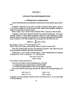
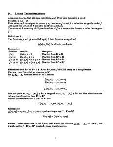
Figure 1: Two 1-D projections of an originally 2-D data that contain two outliers. The PCA projection is fooled by the outliers, unlike the normalized PCA projection that maintains much of the structure of the data. distances. In many cases, this preference impairs the results of PCA. One of the most undesirable consequences of this behavior is the dramatic sensitivity of PCA to outliers (extreme observations that are well separated from the remainder of the data), which are common in realistic datasets. Since pairwise distances involving outliers are significantly larger than the other pairwise distances, PCA emphasizes these outlying distances, thus skewing the projection from the desired one. We illustrate this phenomenon in Fig. 1, in which we present a 2-D dataset, comprised of a bulk of 50 normally-distributed points as well as two outlying points. As can be seen in the figure, the 1-D projection computed by PCA projects the data in a direction that emphasizes the outliers while hiding almost all the structure of the bulky region. We propose a weighted PCA scheme that achieves impressive robustness towards outliers, by normalizing squared pairwise distances in a way that reduces the dominance of the large distances. Specifically, we choose the weights in (5) as: di j =
1 . disti j
The resulting projections are well balanced, aiming at preserving both large and small pairwise distances. We have found this method, which we call normalized PCA, to be superior to the bare PCA, especially when the data contain outliers. For example, refer again to Fig. 1 where the 1-D projection achieved by normalized PCA is demonstrated to preserve much better the overall structure of the data set.
Normalized PCA
As we have shown in Proposition 3.1, PCA strives to preserve squared pairwise distances. The fact that the distances are squared gives a substantial preference to the preservation of the larger pairwise distances, frequently at the expense of preserving the shorter
3.2
Projecting labeled data
When the data is labeled (i.e., clustered), a projection is often required to reflect the discrimination between the clusters. PCA may fail to accomplish this, no matter how easy the task is, as it is an
• For α �= β , the direction vectors are orthogonal:(vα )T vβ = 0. This prevents a situation where two direction vectors are equal or very similar, resulting in ”wasted”, uninformative direction vectors.
85
80
Orthonormality, then, is very important for obtaining proper embeddings. Hence, we cannot just remove this constraint without proposing a suitable replacement. Here, we suggest to relax the orthonormality constraint by posing the more general constraint, enforcing the direction vectors to be B-orthonormal for some properly chosen m × m matrix B, so:
y−coordinate
75
70
weighted PCA
65
(vα )T Bvβ = δαβ ,
60
55
50
PCA
50
55
60
65
70 75 x−coordinate
80
85
90
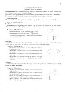
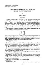
Figure 2: Two 1-D projections of 2-D data that contain two clusters. The PCA projection merges the clusters, while the weighted PCA projection keeps them much apart.
unsupervised technique not designed to handle such cases. It is just that directions that maximize the scatter of the data, might not be as adequate to discriminate between clusters. Fortunately, our generalization to PCA can straightforwardly address labeled data. Assume we are given some dissimilarity values, which might be those used in normalized PCA or simply uniform constants. Then, we may put an emphasis on clusters separation by decaying the weights of intra-cluster pairs, using some decay factor 0 � t � 1, so that the new weights are: � dilabeled = j
t · di j di j
i and j have the same label otherwise
Typically, we take t = 0, which means that we are not interested at all in separating elements within the same cluster. We give an example in Fig. 2, where a 2-D dataset comprising two normally-distributed clusters (200 points each) is shown, together with two 1-D projections. As is well demonstrated, the 1-D PCA projection completely merges the clustering, whereas by setting all the intra-cluster dissimilarities to zero, we obtain a 1-D projection that clearly captures the clustering decomposition.
4
General Linear Transformation
So far we limited ourselves to projections, which are only a specific subfamily of linear-transformations. Recall that projection is achieved as long as the direction vectors are orthonormal. In several cases it would be better to relax this orthonormality restriction and allow other kinds of linear transformations, which are not strict projections. In order to introduce a formal framework of such transformations, let us first dwell upon the implications of the orthonormality: • For every 1 � α � p, the direction vectors are normalized: �vα �2 = 1. This determines the scale of the embedding and is of utmost importance. If we have not restricted the norm of the direction vectors, we could maximize (5) by arbitrarily scaling up the embedding, regardless of its merits. This, of course, makes no sense at all.
α , β = 1, . . . p .
This way we significantly increase the freedom in choosing a linear transformation, yet still maintaining a version of the two aforementioned orthonormality implications. Needless to say, taking B as the identity matrix restores the original orthonormality constraint. In the rest of this section, we describe several suitable choices of the matrix B.
4.1
Achieving orthonormal embedding coordinates
A reasonable requirement from the embedding is that its coordinates would be orthonormal. As the columns of X are centered, so are the embedding coordinates. Orthogonality constraint on the latter, thus, means that they are uncorrelated (two centered vectors are uncorrelated when they are orthogonal) and consequently each axis conveys a new information that does not exist in the rest of the axes. To sharpen the distinction, unlike projection methods, which are characterized by orthonormal direction vectors, here we require the embedding coordinates to be orthonormal. Formally, recall that given direction vectors v1 , . . . , v p ∈ Rm , the embedding coordinates are Xv1 , . . . , Xv p ∈ Rn . Hence we require that for each α , β , (Xvα )T Xvβ = δαβ . This is, (vα )T X T Xvβ = δαβ , meaning that the direction vectors are required to be X T X orthonormal. To summarize, a suitable choice for the matrix B, which ensures uncorrelation between the embedding coordinates, is taking B = X T X. Using lemmas 2.1 and 2.2, we immediately obtain that the solution of � � p 2 (6) max ∑ di j disti j v1 ,...,v p i< j
subject to: (vα )T X T Xvβ = δαβ ,
α , β = 1, . . . p
(7)
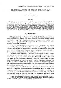
are the p highest generalized eigenvectors of (X T Ld X, X T X). The X T X orthonormality constraint (7) implies (Xvα )T Xvα = 1, which means that the variance of each of the embedding coordinates is 1. Intuitively, this imposes a compromise between the desire to maximize the weighted sum of the squared pairwise distances, and the desire to keep the scatter of the data fixed. As a consequence, this method is perfectly suitable for dealing with labeled data, where intra-cluster dissimilarities have been decayed. In this case we expect highly dissimilar elements (belonging to different clusters) to be placed distantly to maximize (6). On the other hand, elements of the same cluster have (almost) no influence on (6) so they are placed closely to satisfy the constraint (7). Interestingly, this method is a generalization of the known Fisher’s Linear Discriminant Analysis that will be discussed in Subsection 4.4. A demonstration of such an embedding is given in Fig. 3. The dataset comprises hand-written digits taken from www.cs.toronto.edu/~roweis/data.html. This dataset contains 39 samples per digit, where a sample is a 20 × 16 bitmap, resulting in 320(= 20 × 16) binary coordinates. In (a) we show a 2D embedding of this 320-D dataset using the method we formerly
0.5 0.4 0.3
y−coordinate
0.2 0.1 0 −0.1
7
0 0 0 0000 000 0 0 0 0 0 0 00 00 00 000 00 0 0 0 0 0 000 0
7 7
7 7 77 77 7 7 7777 7 7 77 77 7 77 77 7 77 7 7 77 7 7 7
4
4.2
33 3 5 33 3333333333 5 55 5 5 5 5 55 555 5 33 3 33 33 3 555 55 3 333 5 533 5 555 55 5 5 5 3 3 55 5 5 6 3 5 5 22 2 6262 6 6 2 6 6 62 6666 6 2 22 22 6 6626 222 62 66 66 6 222662 62 6 2 22222 2 6 2 6 26 6 66 2 6 2262 2 6 22 6
−0.2 −0.3
44 4 4 4 4 4 4 44 4 44 4 444 4 4 4 44 44 4 444444 44 4 4 44
8 8 8 88 8 8 88 88 88 8 88 88 88 88 8 88888 88 88 8 88
3
33
idating our success in incorporating the dissimilarities into the final result. Unlike the nonlinear eigenprojection, here the embedding axes are interpretable linear combinations of the original descriptors, indicating which characteristics (data coordinates) influence the way people sense different colas.
9 99 999 99 9 9 999 9 9 9 9999 9 9 9 999999 9 9 99 9 9 99 9
Working with similarities
Constraining the direction vectors to be X T X orthonormal makes it feasible to use another approach based on similarities. We define pairwise similarities si j that measure how important it is to place elements i and j close to each other. In analogy with (6) and (7), we can now define the complementary minimization problem:
1 1 1 1 1 1 11 1111 1111 11 11 1 11 1 1 1 11 1 111 1 1 11 1 1
−0.4 −0.5 −0.4
1
min
−0.3
−0.2
−0.1
0
0.1 0.2 x−coordinate
0.3
0.4
0.5
0.6
v1 ,...,v p
∑ si j
� � p 2 disti j
(a)
(8)
i< j
subject to: (vα )T X T Xvβ = δαβ ,
α , β = 1, . . . p
8
1 11
1 1
6 1 111
11 1
1 11
1
1
1 1
1
4
y−coordinate
2
1
1
1
1 4
0 1
6
−2
−4
−6 −10
−8
7
−6
7 7
9
1
7 7 3 7 79 99 1 1 1 3 3 88 1 9 8 7 2 38 1 322 3 83 3 3 3 8 8 8 1 8 822 1 738 8 3 281852 28 3 183 93 39 3 2 8 2 82 22 5 2 3 2 2 8 5 8 8 5 8 9 23 2 5 82 584528 32 8 9 3 1 5 2 0 3 85 3 2 34 8 9 0 55 39 3838 2 5 5 9 9 2 4 8578 6 2 86 2 53 5 8 9 2 45 23 2 0 45 5 858 5 25 2 2 5 55 58 5533 5 4 5 3 9 64 4 2 4 5 3 4 0 4455 5 9 5 5 4 40 4 46 4 2 0 53 4 2 4 4 4 0 440 0 4 00 5 0 4 0 0 0 4 0 0 04 6 6 40 0 0 0 00 0 6 0 0 64 4 6 6 4 0 40 0 6 00 0 0 4 440 60 0 6 64 4 6 666 6 6 66 6 6 6 0 6 6 6 6 6 64 6 6 66 6 6 6 1
1 1
Here we strive to shorten the distance between highly similar elements. It is important to keep in mind that when working with similarities the fixed variance constraint (achieved by the X T X orthonormality) is essential. Otherwise, we might minimize (8) by projecting the data along an uninteresting direction where they have almost no variability. By defining the Laplacian Ls as: � n ∑ j=1 si j i = j Lisj = i �= j −si j
−4
2
−2 x−coordinate
3 3
8
0
2
9
7 7 77 7 7 7 7 7 7 77 77 7 9 9 2 7 9 2 7 7 9 9 9 9 99 97 7 9 3 999 9 97 9 9 7 9 8 7
3 7 7 73 77
9
4
6
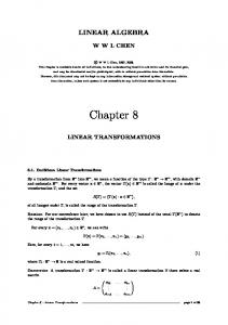
(b) Figure 3: Hand-written digits dataset containing 390 samples in 320-D. (a) Result of our method with good separation of clusters. (b) Result of PCA with poor cluster discrimination
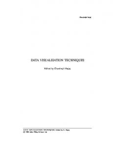
described here. Inter-cluster dissimilarities were simply set to 1, whereas intra-cluster dissimilarities were set to 0, yielding a good separation between clusters. For comparison, we show in (b) the uninformative embedding obtained using PCA projection. Another demonstration of the method is the Colas data taken from [10]. This data was collected in an experiment where tastes of ten colas were compared by a human panel. Subjects were asked to perform two tasks: rate each individual cola with regard to 13 flavor descriptors and to rank the level of dissimilarity between each pair of colas. At the end of the day, the resulting dataset contains ten elements in 13-D space, as well as pairwise dissimilarities. We provide three 2-D embeddings of this dataset in Fig. 4. In (a) we show the embedding computed by PCA. This embedding reflects well the coordinates alone, but cannot account for the dissimilarities between the colas. An embedding of the data using eigenprojection is shown in (b). This embedding accounts for the given pairwise dissimilarities but completely ignores the coordinates. In (c), we use our method with the weights di j being the given dissimilarities, utilizing thereby all available information: coordinates and dissimilarities. Comparison of this embedding to the former two shows a clear resemblance to the nonlinear eigenprojection embedding, val-
and using lemmas 2.1 and 2.2, we can show that (8) is solved by the p lowest generalized eigenvectors of (X T Ls X, X T X). Similarity values appear frequently in data analysis. Two simple ways of extracting them from the coordinates are by using decreasing functions of the distances or by computing correlation coefficients. Sometimes it is beneficial to neglect low similarity values by setting them to zero. The resulting Laplacian will be sparse, having non-zero entries only between close elements. In this case, it is sometimes advisable to set all these non-zero entries to the value 1, thus getting a binary similarity matrix. The similarity-based approach can also be used for labeled data. Here, we have to decay all the similarities between elements from different clusters, using some decay factor 0 � t � 1: � si j i and j have the same label labeled = si j t · si j otherwise Typically, we set t = 0, meaning that we do not want the embedding to reflect any proximity relations between elements from different clusters. We can not give a conclusive advice on whether to prefer working with similarities or with dissimilarities. In general, it depends on which kind of relationships is easier to be measured on the specific data. An example where working with similarities is convenient is the odors dataset shown in Fig. 5. The dataset comprises 30 volatile odorous pure chemicals that were chosen to represent a broad range of chemical properties. The odor-emission of each sample was measured using an electronic nose, resulting in a 16-D vector representing that sample. In total, we have performed 300 measurements to yield a dataset of 300 elements in 16-D that are partitioned into 30 clusters. In a separate work [1], we have developed a technique to derive from the raw data pairwise similarity values between any two samples. In 5(a) we show a 2-D embedding of this dataset using our method, where inter-cluster similarities were set to zero. In general,
0.4 0.2
0.4 0.2
3 2
Diet Pepsi
0
0
RC Cola
−0.2
1
Yukon
Shasta
−0.4
0
−0.4
−0.2
Dr. Pepper
−1
−0.6
Coca−Cola
−0.8
Tab
−1
−0.8
−2
−0.6
Diet Dr. Pepper
Pepsi Cola
(a)
(b)
−0.5 −1.2
−0.4
−0.3
−0.2
−0.1
0
0.1
0.2
0.3
−0.8 −1
−0.6
−0.4
−0.2
0
0.2
0.4
0.6
−1.5 −3
−1
−0.5
0
0.5
1
1.5
Diet Rite
(c)
Figure 4: Three embeddings of the colas dataset. Each is characterized by 13 coordinates reflecting its flavor as assessed by human subjects. These subjects also produced pairwise dissimilarities between the different colas. (a) A PCA projection of the dataset accounting only for the coordinates. (b) Nonlinear embedding by eigenprojection, accounting only for the dissimilarities. (c) A linear transformation by our method, taking into account both coordinates and dissimilarities.
the clusters, which are color-coded in the figure, are well separated. For comparison, we show in (b) the projection of this dataset using PCA, in which case the separation between the clusters is much less significant.
3000
2000
Inter-cluster repulsion and intra-cluster attraction
We have shown in Lemma 3.1 that the matrices X T Lu X and X T X are identical up to multiplication by a positive constant. Consequently, in problems (6) and (8) we can replace the matrix X T X with X T Lu X without altering the solution. This suggests a generalization of these problems by using a general Laplacian, Ld , rather than Lu , in the constraint. Consequently, if we are given pairwise similarities si j , as well as pairwise dissimilarities di j , we may formulate the following minimization problem: � � p 2 min ∑ si j disti j v1 ,...,v p i< j (9) β
subject to: (v ) X L Xv = δαβ , T d
−3000 −2000
−1500
−1000
−500 x−coordinate
0
500
1000
(a) 4 3
1 0 −1 −2
� p 2 ∑i< j si j disti j � � p 2 ∑i< j di j disti j
subject to: (vα )T X T Ld Xvβ = C · δαβ
−2000
2
�
min
−1000
α , β = 1, . . . p
The solution of this problem is given by the p lowest generalized eigenvectors of (X T Ls X, X T Ld X). In order to gain some intuition on (9), we shall rewrite it in the equivalent form:
v1 ,...,v p
0
y−coordinate
α T
1000 y−coordinate
4.3
−3
(10)
α , β = 1, . . . p ,
where C is an arbitrary scaling constant. Since(vα )T X T Ld Xvα = ∑ni< j di j · ((Xvα )i − (Xvα ) j )2 , the last constraint states that the weighted sum of squared distances should be uniform along all axes. It is straightforward to show that a solution of (9) is also a solution of (10). Minimizing the target function of problem (10) is achieved by both minimizing the distances between highly similar elements (to
−4 −5 −4
−2
0
2 4 x−coordinate
6
8
10
(b) Figure 5: Odors dataset containing 300 measurements classified into 30 clusters; color-coding shows the classification. (a) The result of our method, clearly exhibiting sharp separation between the clusters. (b) The result of PCA.
max
v1 ,...,v p
� � p 2 ∑i< j di j disti j � � p 2 ∑i< j si j disti j
subject to: (vα )T X T Ls Xvβ = C · δαβ
(11)
α , β = 1, . . . p
Here, the solution is given by the p highest generalized eigenvectors of (X T Ld X, X T Ls X). Problems (9)–(11) allow for more degrees of freedom than the previous methods discussed in this paper. They let us use pairwise weights not only in the target function that has to be maximized/minimized but also in the orthonormality constraint. Therefore, they are very suitable for labeled data, as they can induce “attraction” between elements of the same cluster, and “repulsion” between elements of different clusters. An important application of these methods is a robust form of Fisher’s Linear Discriminant Analysis, to which we now turn.
4.4
Normalized LDA
A classical and well-known approach for achieving a linear transformation that separates clusters is Fishers’s Linear Discriminant Analysis (LDA) and its generalizations. For details refer to, e.g., [4, 11]. Briefly, the objective of this method is to find the best linear combinations of the data coordinates so as to maximize the inter-cluster variance and minimize the intra-cluster variance. Interestingly, it can be shown that problem (6) (and of course (11)) is a generalization of LDA, as we can choose the dissimilarities such that (6) coincides with LDA, by taking: 1 1 − n·n i and j are both in cluster c n2 c di j = 1 i and j are in different clusters , n2 Here, we denote the number of elements in cluster c by nc . More details will be given in the extended version of this paper. The original and most common use of LDA is for classification, rather than for visualization. When used for visualization it suffers from two drawbacks. First, a simple maximization of the intercluster variance is sensitive to outliers and therefore LDA prefers showing few remotely located clusters while masking closer clusters. For example, in Fig. 6 we show a 2-D dataset decomposed into 10 clusters, each of which contains 100 elements. Two of the clusters are placed distantly from the rest. As can be seen in the figure, the LDA 1-D projection of the data shows clearly the two “outlying” clusters, but completely masks the other eight clusters, which might be the more fundamental portion of the data. The second, more severe problem is that by trying to minimize the variance of a cluster we completely ignore its shape and size. No matter if the cluster is dense or heterogeneous, or if the cluster is elongated or spherical, LDA strives to embed it as a small sphere. This may be good for classification, but prevents a reliable visual assessment of the cluster properties. For a concrete example, consider Fig. 7. This figure shows a 2-D dataset containing two normally-distributed clusters, each of which contains 200 elements. One cluster is symmetric having the same variance along both axes, whereas the other cluster is elliptic, and its variance along the x-axis
60
40
20
Fisher’s LDA
0 y−coordinate
minimize the numerator) and maximizing the distances between highly dissimilar elements (to maximize the denominator). When the data is labeled we decay inter-cluster similarities and intracluster dissimilarities, usually setting them to zero. Consequently, in problem (10) we strive to minimize the weighted sum of intracluster squared distances while maximizing the weighted sum of inter-cluster squared distances. Similarly, we can generalize the maximization problem (6), and obtain the following problem:
−20
−40
−60
−80 normalized LDA −100 −80
−60
−40 −20 0 x−coordinate
20
40
Figure 6: Two 1-D projections of 2-D data composed of ten clusters, two of them are outliers. The LDA projection, striving to maximize the inter-cluster variance, emphasizes only the outlying clusters. However, the normalized LDA separates those eight clusters that form the main trend of the data.
is 10 times larger than the variance along the y-axis. The 1-D projection of LDA makes the two clusters look the same, striving to diminish the intra-scatter of each of the clusters. This way, the heterogeneity of the elliptic cluster cannot be discerned. The two aforementioned shortcomings of LDA can be addressed by an appropriate choice of the pairwise similarities/dissimilarities in our weighted methods. Here we would like suggest a particular weighting scheme, which we call normalized LDA. Similarly to our proof of proposition 3.1, it can be shown that LDA strives to maximize the ratio between inter-cluster pairwise squared distances and intra-cluster pairwise squared distances. Consequently, it is mainly concerned with the larger pairwise distances. This explains why in Fig. 7 it preferred a projection that closely places the distant points of the elliptic cluster. This also explains why LDA prefers separating remotely located clusters. To remedy these shortcomings we suggest to compute the embeddings by optimizing problem (11) with appropriately chosen normalization weights that reduce the dominance of large distances. This is achieved by setting the similarities and dissimilarities as follows: � 0 i and j have the same label di j = 1 otherwise disti j � si j =
1 disti j
0
i and j have the same label otherwise
The normalized LDA is far more robust with respect to a few outlying clusters, corresponding to large distances from the rest of the data. Such distances will have smaller impact as their weights are reduced. This is beautifully demonstrated in Fig. 6 where the 1-D projection of the normalized LDA captures well the eight clusters in a row, reflecting the main trend in the data. Similarly, it is not very important for normalized LDA to place distant points of the same cluster in close proximity, as their respective weights are small. This can be seen in the normalized LDA 1-D projection in Fig. 7, where the different structure of the clusters is preserved, without ruining their separation.
6
Conclusions
10
5
y−coordinate
0
−5
−10
−15
−20
Fisher’s LDA
80
normalized LDA
85
90
95
100 105 x−coordinate
110
115
120
125
Figure 7: Two 1-D projections of 2-D data composed of two clusters of very different shapes. The LDA projection, striving to diminish the intra-cluster variance, produces very similar projections for both clusters. However, the normalized LDA succeeds in showing the different intra-structure of the clusters.
LDA can produce at most k − 1 embedding axes, where k is the number of clusters. On the other hand, normalized LDA can produce m different embedding axes, regardless of the number of clusters (recall that m is the dimensionality of the data). This is yet another advantage of normalized LDA over LDA, which is particularly important in the frequently encountered two clusters problems. In these cases LDA can produce only one-dimensional embedding, while normalized LDA can produce a higher dimensional embedding.
We propose a family of novel linear transformations to achieve low dimensional embedding of multivariate data. These transformations have a significant advantage over other techniques in their ability to simultaneously account for many properties of the data such as coordinates, pairwise similarities, pairwise dissimilarities, and their clustering decomposition. Therefore, we exhaust all kinds of available information so as to make an instructive and reliable visualization. In fact, the derivation of these transformations integrates two apparently very different approaches: those that are coordinatesbased and those that are pairwise-weights-based. This reveals interesting inter-relationships between the linear PCA and LDA and the nonlinear eigenprojection and MDS. Our methods contain PCA and LDA as special cases, but offer more powerful variants that can better visualize the data. Such two interesting variants, which address several shortcomings of PCA and LDA, are normalized PCA and normalized LDA. One of their advantages is an improved ability to handle outliers in the data. All formulations lead to optimal solutions that can be directly computed by eigenvector decomposition of m × m matrices, where m is the dimensionality of the data. This is also the case in PCA and LDA. However, the power of our formulations lies in the fact that these m × m matrices are derived by matrix multiplications that involve an n × n Laplacian matrix, where n is the number of data elements (typically, n >> m). Therefore, we fine-tune the m × m matrix by appropriately altering the n × n entries of the Laplacian. Consequently, the pairwise relationships between data elements are directly reflected in the m × m matrix. One of the most important properties of our methods is that they can adequately address labeled data by capturing well the intercluster structure of the data, as well as the intra-cluster shapes. This is naturally highly beneficial when we are interested in data exploration.
References 5
Relation to Eigenprojection
Interestingly, the methods surveyed here have intimate relationships with the non-linear eigenprojection visualization technique [5, 7, 8]. There, we use only pairwise relationships without utilizing the coordinates themselves. In fact, our methods reduce to the eigenprojection when we discard the coordinates matrix X, by setting it to the n × n identity matrix. To make this apparent, substitute X = I in problem (6) (or (5)) and see that the embedding coordinates would be the p highest eigenvectors of Ld . Similarly, when substituting X = I in (8) the embedding coordinates would be the p lowest eigenvectors of Ls . Such nonlinear embeddings are exactly the results of the eigenprojection method. We have chosen to derive our methods as a generalization of PCA (or LDA), but we could equally well present them as a way to use the eigenprojection for computing linear transformations of the coordinates. By this, we introduce an interesting link between two seemingly unrelated approaches: PCA and eigenprojection. The eigenprojection involves eigenvector computation of an n × n matrix, whereas our methods solve m × m eigen-equations. Typically m is much smaller than n. Therefore, an alternative viewpoint of our methods is as an approximation of eigenprojection that vastly accelerates the computation speed. This approximation computes the optimal embedding only in the m dimensional subspace spanned by the data coordinates, instead of optimizing it in the full n-dimensional space.
[1] L. Carmel, Y. Koren and D. Harel, “Visualizing and Classifying Odors Using a Similarity Matrix”, Proc. 9th International Symposium on Olfaction and Electronic Nose (ISOEN’02), Aracne, pp. 141–146, 2003. [2] G. S. Davidson, B. N. Wylie and K. W. Boyack, “Cluster Stability and the Use of Noise in Interpretation of Clustering”, Proc. IEEE Information Visualization (InfoVis’01), IEEE, pp. 23–30, 2001. [3] G. Di Battista, P. Eades, R. Tamassia and I.G. Tollis, Graph Drawing: Algorithms for the Visualization of Graphs, Prentice-Hall, 1999. [4] B. S. Everitt and G. Dunn, Applied Multivariate Data Analysis, Arnold, 1991. [5] K. M. Hall, “An r-dimensional Quadratic Placement Algorithm”, Management Science 17 (1970), 219–229. [6] M. Kaufmann and D. Wagner (Eds.), Drawing Graphs: Methods and Models, LNCS 2025, Springer-Verlag, 2001. [7] Y. Koren, L. Carmel and D. Harel, “ACE: A Fast Multiscale Eigenvectors Computation for Drawing Huge Graphs”, Proc. IEEE Information Visualization (InfoVis’02), IEEE, pp. 137–144, 2002. [8] Y. Koren, “On Spectral Graph Drawing”, Proc. 9th International Computing and Combinatorics Conference (COCOON’03), LNCS, Vol. 2697, Sringer-Verlag, pp. 496–508, 2003. [9] A. Morrison, G. Ross and M. Chalmers, “A Hybrid Layout Algorithm for Sub-Quadratic Multidimensional Scaling”, Proc. IEEE Information Visualization (InfoVis’02), IEEE, pp. 152–158, 2002. [10] S. S. Schiffman, M. L. Reynolds and F. W. Young, Introduction to Multidimensional Scaling: Theory, Methods and Applications, Academic Press, 1981. [11] A. R. Webb, Statistical Pattern Recognition, John Wiley and Sons, 2002.