Abstract: In this paper the methodology of biplots is introduced as a means for monitoring the behaviour of process systems. This sophisticated methodology ...
VISUALIZATION OF PROCESS DATA WITH BIPLOTS Sugnet Gardner,§ Niel J. Le Roux,§ and Chris Aldrich* §Department of Statistics and Actuarial Science, University of Stellenbosch, Stellenbosch, Private Bag X1, Matieland, 7602, Stellenbosch, South Africa. *Institute of Mineral Processing and Intelligent Process Systems, Department of Process Engineering, University of Stellenbosch Stellenbosch, Private Bag X1, Matieland, South Africa 7602 Fax +27(21) 808 2059
Abstract: In this paper the methodology of biplots is introduced as a means for monitoring the behaviour of process systems. This sophisticated methodology allows for the projection of high-dimensional data to a low-dimensional subspace that can be visualised by a human operator. The projections are highly graphical in nature, and rich in information regarding variation in process variables, correlations among these variables, as well as class separation, taking into account the multivariate character of the data. Moreover, as is shown by way of two case studies, process disturbances can be visualised and explored quantitatively by superimposing alpha-bags on biplots. Keywords: Biplot, Process Control, Modelling, Hydrometallurgy, Froth Flotation.
1. INTRODUCTION Process data are used extensively in modern industrial environments for monitoring product quality, control and optimization. Large volumes of data are routinely collected and stored on many plants and in order to exploit the data to get a better understanding of the behaviour of the process, it is important to identify the salient features underlying the data. By reducing the dimensionality of the problem, the engineer is able to summarize the information captured in a large number of variables by a smaller number of latent variables. Principal component analysis (PCA) is by far the most important technique used for this purpose, and is widely supported by statistical software. As is indicated in this paper, PCA can be extended with modern biplot methodology by providing a single graph for displaying the variation in multidimensional observations, together with information on all variables concerned. Canonical variate analysis (CVA) biplots on the other hand, are ideally suited for optimally separating classes of observations. Biplots provide an infrastructure for implementing many novel ideas in monitoring industrial plant processes and allows for non-linear relationships among process variables. 2. BIPLOT METHODOLOGY A biplot is a graphical display consisting of a vector for each row and a vector for each column of a matrix of rank two (Gabriel, 1971). The elements of the matrix are represented by the inner products of the vectors corresponding to their rows and columns. Since any matrix of rank k > 2 can be approximated
by a matrix of rank two, a biplot can be constructed for all matrices by considering its rank two approximation. Although the traditional Gabriel biplot is widely applied as a graphical aid in practice, biplots can also be viewed as multivariate analogues of scatterplots that are easy to interpret (Gower, 1995; Gower and Hand, 1996). In regarding the biplot as a multivariate extension of an ordinary scatterplot the focus is on representing interpoint distances. Since scatterplots have the merit of being familiar, requiring very little formal training to interpret, this biplot is accessible to non-statistical audiences. The multidimensional observations are represented by points in a two-dimensional display while variables are represented as biplot axes – for each variable a separate axis. Furthermore, these (non-perpendicular) axes are calibrated in the original scales of measurement so as to be used in much the same way as the two perpendicular axes of a scatterplot. Mathematically, the process of finding the coordinates of the original points in the PCA biplot space amounts to performing a singular value decomposition of the data matrix consisting of n observations on p variables. However, these axes are not shown but form the scaffolding for constructing the biplot. The relationships between the scaffolding and the original variables are termed interpolation and prediction (cf. Gower & Hand, 1996). For a given or a new observation, interpolation is the process of finding its representation in the biplot space. Prediction, on the other hand, is inferring the values of the original variables in terms of the biplot scaffolding. Thus, what is shown in a PCA biplot are the observations and a set of axes, calibrated in the original units, representing the variables. It can be shown that two different sets of axes are needed: one
set for interpolation and another for prediction. Since it is natural to use axes for inferring values of the observations for the different variables, only prediction axes will be fitted to biplots shown here. Interpolation is usually performed by a suitable computer programme. CVA aims to find the linear combination of the predictor or discriminatory variables that maximises the ratio of the between groups to within groups variance. This process amounts to transforming the original means to a new set of means, known as canonical means. The statistical (Mahalanobis) distances in the observation space become ordinary Euclidean distances in the canonical space. Mathematically, the process of finding the coordinates of the original points or means in the canonical space amounts to solving a two-sided eigenvalue problem leading to a set of axes for constructing a biplot.
less than 5 M. Under these conditions, three phases of zinc chloride can occur, viz. Zn(NH3)2Cl2 , Zn(OH)2 and Zn(OH)1.6Cl0.4. Of the 108 samples, 22 were associated with the precipitation of Zn(NH3)2Cl2, 37 with and 43 with Zn(OH)2 and Zn(OH)1.6Cl0.4, while six samples consisted of mixed precipitates, i.e. three observations associated with Zn(NH3)2Cl2-Zn(OH)1.6Cl0.4 and three observations associated with Zn(OH)2-Zn(OH)1.6Cl0.4. TEMP 70
60 NH3
1.6 1.4
50 1.2 1 0.6 0.6 0.8
Moreover, by adding alpha-bags to a CVA biplot a quantitative measurement of multidimensional overlap or separation of groups can be obtained, thereby providing information not only about the degree of overlap, but also the nature of the overlap. Gardner (2001) proposed the alpha-bag for characterising a two-dimensional cloud of points as well as for quantifying overlap among classes. Although trivial to rank univariate data according to a single criterion e.g. length, the process of ranking multivariate data is far from trivial. Tukey (1975) and Rousseeuw, Ruts & Tukey (1999) discussed the concept of halfspace location depth as a means of generalising the univariate rank concept to a bivariate data set. This concept forms the basis of the alpha bag that encloses the exact innermost α% of bivariate data points as specified by the user. The resulting contours are called alpha-bags and are proposed as summaries of data points in two dimensions. 3. HYDROLYSIS OF ZINC CHLORIDE IN AMMONIUM CHLORIDE SOLUTIONS Since aqueous solutions of high concentrations of ammonium chloride are especially appropriate for the treatment of complex raw materials of both oxide and sulphide types, hydrometallurgical processes using ammonium chloride have generated considerable interest in recent years (Figueiredo et al., 1993; Limpo et al., 1992). Process development cannot take place without a detailed knowledge of the solubility of metal chlorides as a function of temperature and composition of solution and in this case study data generated by Limpo et al. (1995) are examined by means of biplots. The data set consisted of 108 samples obtained from an experiment where zinc chloride is hydrolysed in a watery ammoniacal-ammonium chloride solution. Four variables were measured, namely the temperature of the solution (ranging from 30-50°C), the concentration of chloride anions (Cl-), the concentration of zinc cations (Zn2+) and the ammonia concentration (NH3). The concentrations were all
1 0.8
1
Zn
5 Cl C
3
0.4 40 0.4
2
0
0.2 0.2
4 30
6 20
10
Fig.1. PCA biplot of the hydrolysis of zinc chloride data set. Figure 1 shows a PCA biplot of this data set. The sample points appear in three horisontal bands corresponding to the three temperature settings. The different precipitates, excluding the six mixed observations, are indicated by different colours. The variation in the values of NH3, Zn2+ and Cl- for each precipitate can be clearly ascertained from the respective calibrated axes. Although the three precipitates can be clearly discerned, the PCA biplot optimally represents the total variation in the observations. Constructing a CVA biplot of this data optimally separates the three classes. Limpo et al. (1995) have found that for chloride concentrations between 3.5 and 5 M, the solubility of the zinc in the ZnCl2-NH4Cl-NH3-H2O system was determined by the solubility of the zinc diammine chloride. For chloride concentrations lower than 3.5 M, there were two zinc compounds, viz. zinc hydroxide and zinc hydroxychloride. They have concluded that the solubility of these two zinc compounds depended on the ratio of the total ammonia concentration to the total zinc concentration, ([NH3]/[Zn]). A much richer presentation of these results can be obtained by projecting the experimental data onto the CVA biplot, as indicated in Figure 2. In this figure, the red, green and blue circles indicate the formation of Zn(NH3)2Cl2, Zn(OH)2 and Zn(OH)1.6Cl0.4 respectively. The alpha-bags delineate the innermost 50% data points within each class. Figure 2(a) shows the CVA biplot with 50%-bags.
regions in Figure 2(b), allows classification of each phase Zn(NH3)2Cl2, Zn(OH)2 and Zn(OH)1.6Cl0.4 with 88.0%, 94.2% and 95.2% correct classifications respectively. The overall correct classification is 93.1%. The mixed precipitates were not included in the construction of the classification map portrayed in Figure 2(b). Table 2 contains the results when these mixed precipitates were classified according to the CVA biplot procedure. In this table the actual phase θ represents Zn(NH3)2Cl2-Zn(OH)1.6Cl0.4, while the phase γ represents Zn(OH)2-Zn(OH)1.6Cl0.4.
44
-0.2
1.5
0 42
Cl
1.0
0.2
1
2
3
0.6
0
4
38
NH3
Table 1: Classification of solid precipitates with linear discriminant analysis.
5 0.8 6
TEMP Zn(NH3)2Cl2
Zn
Zn(OH)2
Zn(OH)1.6Cl0.4
(a)
42
Cl
Temp (°C) 40 40 40 30 30 30
1.0
0.2
1
2 0.4 3
4
0.6
0 38
NH3
Actual Phase Zn(OH)2 Zn(OH)1.6Cl0.4 0 0 33 2 2 40
88.0%
94.2%
95.2%
[Cl-] (M) 3.97 4.07 3.48 2.28 2.29 2.27
[Zn2+] (M) 0.766 0.804 0.541 0.209 0.294 0.233
[NH3] (M) 0.872 0.867 0.767 0.250 0.890 0.676
Actual Phase θ θ θ γ γ γ
Classification Zn(NH3)2Cl2 Zn(NH3)2Cl2 Zn(NH3)2Cl2 Zn(OH)2 Zn(OH)2 Zn(OH)2
5 0.8 6
TEMP Zn(NH3)2Cl2
Zn(NH3)2Cl2 22 2 1
Table 2: Classification of the out-of-sample mixed precipitates with the CVA biplot classification procedure.
1.5
0
Predicted Phase Zn(NH3)2Cl2 Zn(OH)2 Zn(OH)1.6Cl0.4 % Correct classifications
Zn(OH)2
Zn Zn(OH)1.6Cl0.4
(b) Fig.2. A CVA biplot and 50%-bags of the hydrolysis of zinc chloride data set. The three classes are separated very well: Although not shown here, the innermost 95% of the bivariate data points in anyone of the classes do not overlap with the 5% most extreme bivariate data points in the remaining two classes. The biplot also indicates fair amounts of variation within classes. Furthermore, it is clear that the formation of Zn(NH3)2Cl2 (red circles) is determined by the chloride concentration [Cl-] in the range 3.5-5 M, while the formation of Zn(OH)2 (green circles) and Zn(OH)1.6Cl0.4 are determined by the ammonia [NH3] and zinc [Zn2+] concentrations when the chloride concentration is below approximately 3.5 M. The centroid of each region is indicated by a solid square. Figure 2(b) shows the CVA biplot equipped with classification regions, while Table 1 is the confusion matrix resulting from performing a CVA biplot classification of the data. It follows from Table 1 that the biplot classification delineating the classification
Using this classification Figure 2(a) also shows the mixed precipitates interpolated into the CVA biplot. These mixed precipitates are shown as three solid red circles (Zn(NH3)2Cl2- Zn(OH)1.6Cl0.4) just outside the 50% region of the Zn(NH3)2Cl2 precipitates (delineated by a solid red line) and three solid green circles (Zn(OH)2-Zn(OH)1.6Cl0.4) distributed across the region of the Zn(OH)2 (delineated by a solid green line). 4. CALCIUM CARBIDE FURNACE Commercial calcium carbide is a grey to reddishbrown crystalline material consisting of a mixture of CaC2 and CaO together with impurities introduced by the charge components during manufacture. When brought into contact with water, carbide produces acetylene gas of high purity in accordance with the equation CaC2 + 2H2O → C2H2 + Ca(OH)2 and it is this property that is largely responsible for its importance as a chemical substance. The volume of acetylene generated is therefore used as a measure of carbide quality in the industry in preference to the percentage CaC2. The volume of gas generated is referred to as the gas yield and is expressed in litres per kilogram at standard conditions of temperature and pressure. The uses of acetylene gas are well known, ranging from a source of illumination when the gas is burned in air to produce a bright white light, to the combustion of acetylene in oxygen to
provide a high temperature heat source for the welding and cutting of metals. Acetylene gas is also the basic material for the synthesis of many organic compounds including solvents, plasticisers, plastics and synthetic rubbers. Calcium carbide is produced by fusing together a mixture of coke (or coal) and lime in an electric furnace according to the reaction CaO + 3C → CaC2 + CO. A data set reflecting process operation over an 8month period was constructed, containing the following variables (monitored daily): FURNLOD = furnace load (ton), POWERCON = power consumption (MWh/ton), RESIST = average resistance underneath the three electrodes (mΩ), CHARCOAL = charcoal consumption (ton), COKE = coke consumption (ton), ANTHRACT = anthracite consumption (ton), LIMUNDER = lime characteristics (% underburnt), LIMOVER = lime characteristics (% overburnt), LIM2O = ratio of % lime underburnt to % lime overburnt, i.e. LIM2O = LIMUNDER/LIMOVER, CARBPROD = carbide production (ton), and CARBGRAD = carbide grade (litre/kg). In Figure 3 a PCA biplot is constructed for displaying the variation in the data for all the process variables simultaneously in a single graph. The multiplication of CARBPROD and CARBGRAD was used to quantify the quality of the product. Observations associated with lower quality product are indicated in red and the observations associated with higher quality in green. Although the PCA biplot does not aim to optimally separate these two classes, the difference is already obvious from this graph with higher quality product corresponding to higher values of FURNLOD, CHARCOAL and ANTHRACT and lower values for RESIST. -5
20
0
3.5
In the first case study, a CVA biplot could be used for visualising the hydrolysis of zinc chloride in ammonium chloride solutions. Different zinc precipitates could be classified in terms of different process conditions and mixed precipitates could then be assigned to the different classes by mapping them to the biplot. In the second case study, a PCA biplot was likewise used to identify different operating regimes in a calcium carbide furnace. Once these operating regimes were defined, process conditions differentiating between the desirable and less desirable regimes could be identified with a CVA biplot and this information could then be used to formulate process control strategies for the plant. Finally, different distance measures can be used with the biplot methodology introduced in this paper. In addition to the PCA and CVA biplots illustrated here, non-linear and generalised biplots can be constructed. These biplots enable users to display observations together with continuous as well as discrete or categorical variables. Moreover, Gardner (2001) has proposed several extensions of biplot methodology in statistical discrimination and classification to provide for non-linear relationships. It follows that biplot methodology is an extremely useful tool for analysing multivariate process behaviour. REFERENCES Aldrich, C. and Reuter, M.A., Monitoring of metallurgical reactors by the use of topographic mapping of process data. Minerals Engineering, 1999, 12(11), 1301-1312.
POWERCON LIMU2O
and CVA biplots to monitor multivariate process systems were demonstrated in two case studies, which focussed on the description of multidimensional variation and the separation of different classes of observations.
0
-4 LIMUNDER
50
16
5
RESIST
17
100
16
-4
12 0
150
10
2
-2 1.8
3 8 15
15
2
4
200
10
0 20
1.6 30
40 50
CHARCOAL
20
6 ANTHRACT
Figueiredo, J.M., Novais, A, Limpo, J.L. and Amer, S., The CENIM-LNETI process for the zinc recovery from complex sulphides. In: Matthew, I.G. (ed.), Proceedings of the International Symposium on World Zinc ’93, AusIMM, Hobart, 1993, pp. 333-339.
350
1.2 8
0 400
8 13
2.5 25
FURNLOD
12
-4
30
12 11 -8
10
35 COKE
LIMOVER
Fig.3. A PCA biplot of the calcium carbide furnace data set. 5. CONCLUSIONS In this paper, biplots resulting from the modern perspective of Gower and Hand (1996) were introduced. In particular, the potential of these PCA
Gardner, S., Extensions of biplot methodology to discriminant analysis with applications of nonparametric principal components. Unpublished Ph.D. thesis, 2001, Department of Statistics and Actuarial Science, University of Stellenbosch, Stellenbosch, South Africa. Gabriel, K. R., The biplot graphical display of matrices with application to principal component analysis. Biometrika, 1971, 58, 453-467. Gower, J.C., A general theory of biplots. In Krzanowski, W.J. (ed.). Recent Advances in Descriptive Multivariate Analysis, 1995, Clarendon Press, Oxford, pp. 283-303.
Gower, J. C. and Hand, D. J., Biplots, 1996, Chapman & Hall, London. Limpo, J.L., Figueiredo, J.M., Amer, S. and Luis, A. The CENIM-LNETI process: A new process for the hydrometallurgical treatment of complex sulphides in ammonium chloride solutions. Hydrometallurgy, 1992, 28, 149-161. Limpo, J.L., Luis, A. and Cristine, M.C., Hydrolysis of zinc chloride in aqueous ammoniacal
ammonium chloride solutions. Hydrometallurgy, 1995, 38, 235-243. Rousseeuw, P.J., Ruts, I. and Tukey, J.W. The bagplot: a bivariate boxplot. The American Statistician, 1999, 53, 382-387. Tukey, J.W. Mathematics and the picturing of data. Proceedings of the International Congress of Mathematicians, 1975, 2, 523-531.