THE JOURNAL OF CHEMICAL PHYSICS 127, 014903 共2007兲
Visualizing the dynamics of complex spatial networks in structured fluids S. Scherdel
Chemische Physik, TU Chemnitz, Reichenhainer Strae 70, D-09126 Chemnitz, Germany
H. G. Schoberth
Physikalische Chemie II, Universität Bayreuth, Universitätsstrae 30, D-95440 Bayreuth, Germany
R. Magerlea兲
Chemische Physik, TU Chemnitz, Reichenhainer Strae 70, D-09126 Chemnitz, Germany
共Received 19 January 2007; accepted 15 May 2007; published online 5 July 2007兲 We present a data reduction and visualization approach for the microdomain dynamics in block copolymers and similar structured fluids. Microdomains are reduced to thin smooth lines with colored branching points and visualized with a tool for protein visualization. As a result the temporal evolution of large volume data sets can be perceived within seconds. This approach is demonstrated with simulation results based on the dynamic density functional theory of the ordering of microdomains in a thin film of block copolymers. As an example we discuss the dynamics at the cylinder-to-gyroid grain boundary and compare it to the epitaxial cylinder-to-gyroid phase transition predicted by Matsen 关Phys. Rev. Lett. 80, 4470 共1998兲兴. © 2007 American Institute of Physics. 关DOI: 10.1063/1.2747598兴 I. INTRODUCTION
Block copolymers and ordered mesophases of surfactants form spatially complex structures on the nanometer scale.1 These materials have attracted a large interest as templates for the synthesis of nanostructures of inorganic materials.2 Furthermore interesting similarities exist to biomembranes3 and intracellular compartments in living cells.4 In the past decade different experimental techniques such as electron tomography5,6 and nanotomography7 have been developed to obtain volume images of these structures with 10 nm resolution. At the same time advances in theory and simulation methods allow us to predict the structure and dynamics of these systems.8 Of particular interest for the understanding of the structure formation processes is the spatial structure of individual defects and grain boundaries and their dynamics during shear flow,9–11 structural phase transitions,13–15 and their behavior in electric fields.6,16–21 The typical simulation result is the spatiotemporal evolution of the density distribution of block copolymer components within the simulated volume. The data set consists of several thousand snapshots of such density distributions 共Fig. 1兲. Figure 1共a兲 shows the density distribution on the boundary of the simulated volume. The task is to also display the internal structure within the simulated volume, to do this for all time frames, and to enable the viewer to perceive the spatially complex structures as well as their temporal evolution. Because of the large number of available time frames, methods are needed which allow for a fast reception of the spatially complex dynamics. The techniques to display threedimensional data sets either with two-dimensional projeca兲
Author to whom correspondence should be adressed. Electronic mail:
[email protected]
0021-9606/2007/127共1兲/014903/6/$23.00
tions or on stereo displays are called volume rendering.12 The conventional approaches to visualize three-dimensional block copolymer microdomain structures are isodensity surfaces 关Figs. 1共b兲 and 1共c兲兴. Because the typical volume fraction of the material is in the 30%–50% regime, meaningfull isodensity threshold values give rather dense networks which obstruct the view into the simulation box. A common way to overcome these visualization problems is to crop the volume and display only small parts of the entire structure.22 An alternative is to display only a two-dimensional cross section through the volume data set23 or to restrict oneself to the study of two-dimensional or quasi-two-dimensional systems.13–15,18,21 A direct volume rendering using an appropriate transparency map12 is also not suitable for an easy reception and recognition of block copolymer microdomain structures in large volumes because of the rather smooth density variations. Alternative representations of microdomain structures are intermaterial dividing surfaces,24 the reduction of microdomains to their skeleton,25 and medial surfaces.26 In this work we present a method for preception of the spatially complex dynamics in block copolymers and other structured fluids. The method consists of two steps. First the microdomain structures are reduced to their minimal features: connections are represented as thin smooth lines and branching points as small spheres of different colors. The resulting network and its dynamics are visualized with a tool for protein visualization. As a result, the viewer can perceive large data streams with hundreds of volume images within seconds when displayed as an animated sequence of images 共movie兲. As an example, we present the dynamics of a transient defect in a thin film of block copolymers simulated with dynamic density functional theory 共DDFT兲.27 The microdomain structures resemble the gyroid-to-cylinder transition predicted by Matsen using self-consistent field theory
127, 014903-1
© 2007 American Institute of Physics
Downloaded 22 May 2008 to 10.1.150.91. Redistribution subject to AIP license or copyright; see http://jcp.aip.org/jcp/copyright.jsp
014903-2
J. Chem. Phys. 127, 014903 共2007兲
Scherdel, Schoberth, and Magerle
FIG. 1. Mesodyn simulation of a A3B12A3 block copolymer film in a simulation box, with film thickness H = 42, interaction parameter ⑀AB = 7.1, surface field ⑀ M = 6.0, and periodic boundary conditions. The surfaces are located at the top and the bottom of the simulation box. 共a兲 Density distribution of the A component after 1600 time steps. Dark corresponds to a high A density. 共b兲 Corresponding isodensity surface for a threshold value A = 0.33. The enclosed volume corresponds to the volume fraction of the A component. 共c兲 Isodensity surface for A = 0.75.
共SCFT兲.28 Our simulation result shows the same structure and orientation of the defect, however, a different dynamics.
II. METHOD A. Visualization
Our visualization approach is schematically shown at a detail 共Fig. 2兲 of a much larger data set 共Fig. 1兲. Starting from the three-dimensional 共3D兲 density distribution of the A component we set the threshold A = 0.33 and obtain the isosurface 关Fig. 2共a兲兴. It encloses all pixels with density values greater than the threshold value. The result is a binarized 3D volume data set which we skeletonize in the next step. For this, different algorithms exist which have been reviewed in Refs. 33 and 34. The algorithms differ in certain features such as robustness, thinness, invariance under isometric transformations, symmetry, efficiency, and homotopy 共see, e.g., Ref. 35兲. We have chosen the algorithm of Tsao and Fu36 which is based on local connectivity and topology and is easy to implement. It iteratively removes so-called simple points until only the skeleton is left. A simple point is a border point whose deletion does not change the topology in its 3 ⫻ 3 ⫻ 3 vicinity. To prevent the removal of surface or curve end points the preservation of topology is also checked in the two 3 ⫻ 3 vicinities of the point which are parallel to the thinning direction and to every one of the other two axes perpendicular to the thinning direction. First, the two-dimensional medial surface which consists of the centers of the maximal balls inscribed into the objects which are skeletonized is computed and subsequently in a second pass the onedimensional medial axis. A drawback of the algorithm is its sensitivity to noise and that it removes voxels only from one particular direction in each pass. Because of this, it is sensitive to the predetermined order of the different directions and hence not rotational invariant. The resulting skeleton is shown in Fig. 2共b兲. Our implementation of the algorithm of Tsao and Fu does not account for the periodic boundary conditions of the original data set and introduces artifacts in about 5 pixels wide zone at the boundary. We have solved this problem by
FIG. 2. 共Color online兲 Illustration of our data reduction and visualization technique. 共a兲 A small piece of isodensity surface displaying a branching cylinder. 共b兲 Medial axis obtained by applying the thinning algorithm of Tsao and Fu. 共Ref. 37兲. 共c兲 Visualization of the data shown in 共b兲 as a stick and ball model. Kinks reflect the discrete points of the medial axis. Balls mark branching points with the color coding of the number of branches. 共d兲 Same as 共c兲 after removal of artifacts, such as clusters of balls. 共e兲 Same as 共d兲 with the branches approximated by a cubic smoothing spline.
enlarging the data set by periodic continuation of 16 pixels in each direction and cropping the resulting skeleton to the original size of the data set. The next step is to transform the skeleton to a stick and ball model 关Fig. 2共c兲兴. To this end we use the data format of the protein database37 共PDB兲 which is a standard for filing of protein structures which can be considered as complex network structures. Due to the noise of A and the discreteness of the data different artifacts exist. The most frequent artifacts are short 共1–2 grid units long兲 protrusions and clusters of threefold branching points at positions where the cylinders branch. Furthermore the connecting lines are irregular. In a first pruning step the short protrusions and clusters 关such as in Fig. 2共c兲兴 are identified and removed 关Fig. 2共d兲兴 by comparing them with an empiric catalog of artifacts. The pruning is done in the following way: 共I兲
Assign to each point 共voxel兲 of the skeleton a value corresponding to its number of neighbors Find a point with at least three neighbors Inspect the values of the neighbors of this point
共II兲 共III兲 共1兲
If there is a neighbor with value of 1 共one voxel protrusion兲 共a兲 共b兲
共2兲
If there are neighbors with value of 2 共a兲 共b兲
共3兲
Check if one of them is connected to another neighbor of the primary point If there is such a pair then delete the neighbor with value of 2 and correct the values of the points neighboring to the deleted point
If there are at least two neighbors with a higher value than 2: Search for two neighbors which are connected to each other 共they form a triangle兲. If such a triangle is found 共a兲 共b兲 共c兲
共4兲
Delete this neighboring point Correct the value of the primary point
Place a new point in the center of the triangle Delete the old triangle and add connections to the new point Set the values of the new point and correct the values of its neighbors
Repeat step 3 until no triangles are found
Downloaded 22 May 2008 to 10.1.150.91. Redistribution subject to AIP license or copyright; see http://jcp.aip.org/jcp/copyright.jsp
014903-3
Visualizing networks dynamics
J. Chem. Phys. 127, 014903 共2007兲
With these pruning steps also more complex examples can be reduced. For illustration of the pruning algorithm see supplementary data.38 At this step the branching points and end points are colored according to the number of branches. Then the irregular connecting lines are smoothed by cubic smoothing splines 关Fig. 2共e兲兴. As we used the PDB format the result can be visualized in 3D with various software tools, for instance 39 PYMOL. A particular feature is its ability to view the 3D data set in stereo mode and anaglyph views. From the series of anaglyph views we have produced movie 1 共see supplementary data38兲. B.
MESODYN
computer simulation
For demonstrating our visualization approach we have used the result of a MESODYN simulation29 similar as in Ref. 27 where the structure formation in a thin film of cylinder forming block copolymer melt is modeled. A3B12A3 block copolymers are modeled as Gaussian chains with different beads A and B. A Gaussian kernel characterized by ⑀AB is used to model the bead-bead interaction potential. The film interfaces were treated as masks 共M兲 with a corresponding bead-mask interaction parameter ⑀ M = ⑀AM − ⑀BM . For the spatiotemporal evolution of bead densities i共r , t兲 the complete free energy functional F关i兴 and the chemical potenials i = F关i兴 / i are used. The Langevin diffusion equation is solved numerically starting from homogeneous densities. An appropriate noise is added to the dynamics. For details on the simulation method see Ref. 30. MESODYN simulations predict correctly the equilibrium structure27,29–32 and the microdomain dynamics13 in thin films of block copolymers. In order to demonstrate our new visualization approach we have chosen a simulation run of a thick film with film thickness of H = 42 grid units and interaction parameters ⑀AB = 7.1 and ⑀ M = 6.0 共both in kJ/mol兲. For details of the parametrization and the resulting equilibrium structures see Ref. 27. The particular simulation run used in this work is a typical result. Different noise and another initialization of the random number generator would cause another dynamics but the same final equilibrium structure. III. RESULTS
As an example to demonstrate our visualization approach we have modeled the structure formation process in a thin film of block copolymer. The simulation result is the density distribution of the two components A and B as a function of space and time. The isodensity surfaces show the change of the microdomain structure from the initially homogeneous distribution to the equilibrium structure of hexagonally ordered cylinders. The rather thick microdomains obstruct the view into the inner parts of the simulated volume 关Figs. 1共b兲 and 1共c兲兴. This makes it difficult to observe the details of structural rearrangement processes. With our data reduction the isosurface is transformed to a network of thin smooth lines with branching points colored by their connectivity order 共Fig. 3 and movie 2 in the supplementary data38兲. Compiling the series of images into a stereo view or anaglyph movie and playing it in a fast mode make it easy to
FIG. 3. 共Color兲 Reduced representation of the network of A cylinders in a thin film of A3B12A3 block copolymers, calculated from an isosurface with threshold value A = 0.33 for 15 000 time steps. The thin lines do not obstruct the view into the simulation box. The complex 3D network structure is much better perceivable in the anaglyph movie 1 共see supplementary data, Ref. 39兲. Three different structures are visible in the simulation box: in the upper third hexagonally orderd cylinders 共C兲, in the middle a gyroid like network 共G兲, and in the lower third layers of perforated lamellae 共PL兲. Our visualization technique allows us to see and follow the 3D dynamics of the network. A characteristic detail of the structure at the cylinder-to-gyroid boundary is marked with thick lines and displayed in Fig. 4共a兲 along with its further dynamics.
percept the block copolymer dynamics over some 10 000 time steps within seconds. The coding of branching points makes it easier to orient within the structure and to recognize characteristic structures and defects. Starting from a homogeneous distribution the two components first microphase separate and form microdomains with no long-range order. This process is finished after about 200 time steps. The next step is the much slower ordering process of microdomains. In the first phase 共200–3000 time steps兲 the microdomains orient parallel in the vicinity of surfaces and form a layer of perforated lamellae at each surface. In the middle of the film the microdomains remain disordered. In the following the order propagates towards the center of the film. This result is similar to the simulation results of Ref. 40 who have first studied with MESODYN simulations the surface induced ordering process in a lamella forming system. We study a cylinder forming system close to the gyroid and perforated lamella phases.27 The ordering process towards hexagonally ordered cylinders involves transient phases such as the gyroid and perforated lamella phases. In addition our particular simulation is complicated by a spontaneous symmetry break into differently ordered phases which we attribute to the fact that the involved phases are energetically similar. At the upper surface cylinders are formed already after 9000 time steps, whereas at the lower surface the perforated lamella remains. In the middle a disordered network of microdomains exists which we consider as gyroidlike because of the large number of threefold connections. The layer of the cylinders next to the upper surface acts as a nucleus for the equilibrium phase
Downloaded 22 May 2008 to 10.1.150.91. Redistribution subject to AIP license or copyright; see http://jcp.aip.org/jcp/copyright.jsp
014903-4
J. Chem. Phys. 127, 014903 共2007兲
Scherdel, Schoberth, and Magerle
FIG. 4. 共Color兲 共a兲 Sequence of microdomain structures during the gyroidto-cylinder transition observed in this work. The corresponding time steps are displayed in the figure. The arrow marks a moving connection, the scissors mark a breaking connection. 共b兲 Sequence of structures during the cylinder-to-gyroid transition predicted by Matsen 共Ref. 29兲. The color coding of branching points is the same as in Fig. 3. Adopted from Ref. 29; ©1998 American Physical Society兲.
of hexagonally ordered cylinders. Starting from this layer the phase grows towards the lower surface. Close to the end 共at 29 000 time steps兲 almost the whole structure has transformed to hexagonally ordered cylinders except for a few defects and two rings of a perforated lamella in the vicinity of the bottom surface. At 34 000 time steps the equilibrium structure of hexagonally ordered cylinders is reached. The situation at 15 000 time steps is shown in Fig. 3. The color coding of branching points reveals that the network structure is mainly built up from threefold connections. Fourfold and fivefold connections are seldom and very short living. This indicates that these defects are energetically very unfavorable. The elementary step of the structural transformation process turns out to be the stepwise breakup and formation of connections between microdomains. An interesting example
for this is the microdomain dynamics at the cylinder-togyroid grain boundary. The corresponding microdomains are marked in Fig. 3 with thick lines. The color coding is introduced to distinguish the different cylinders in the 2D projection. The cylinders orient in layers parallel to the upper surface. At the boundary to the gyroidlike phase the threefold branching points which bridge cylinders in neighboring layers are characteristic for the gyroid structure. In Fig. 4共a兲 the temporal evolution of this structural feature is shown. The transformation proceeds via stepwise breaking and forming of connections of microdomains. For instance, one of the black cylinders shown in Fig. 4共a兲 moves along the purple arrow by first breaking up in the vicinity of the threefold connections 共t = 17 000兲 and then connecting to the neighboring threefold connection and forming a fourfold branching at t = 17 750. At a later stage this fourfold branching breaks up stepwise starting at the position marked by the purple scissors. During the transformation process a fourfold and a fivefold connection appear but only for a very short period of time. This example shows how with our visualization technique an interesting process can be identified in the center of the simulation box. It is important to keep in mind that the original data set is the dynamics of a density distribution. Therefore we now return to a representation of the data which is better suited to display the details of a continuous density distribution. Figure 5 shows the density distribution in the plane defined by the cylinders marked in Fig. 3 with thick black lines together with the isosurface of these cylinders. The dynamics is best seen in the corresponding movie 共movie 2 in the supplementary data38兲. The sequence of snapshots shown in Fig. 5 illustrates the stepwise breaking and forming of connections between cylinders described above and shown in Fig. 4. In addition to the skeleton of the cylinders this representation reveals details of the density distribution such as the thinning of breaking connections, the thickening of open ends, and density modulations along the microdomains which belong to the gyroidlike structures. The structures at the intermediate steps resemble characteristic structural features predicted by Matsen who has studied theoretically the gyroid-to-cylinder transition with self-consistent field theory 关Fig. 4共b兲兴.29 IV. DISCUSSION A. Visualization method
We have demonstrated our method on block copolymer micordomain structures forming cylinders, perforated lamellae, and gyroidlike structures. These structures represent a large part of the mesophases in block copolymers and surFIG. 5. 共Color online兲 关共a兲–共e兲兴 Snapshots of movie 2 共see supplementary data, Ref. 39兲 showing the dynamics of the A density in the plane defined by the thick black lines shown in Figs. 3 and 4共a兲. Light 共dark兲 green corresponds to a low 共high兲 A density. In addition the isodensity surfaces 共gray兲 are shown.
Downloaded 22 May 2008 to 10.1.150.91. Redistribution subject to AIP license or copyright; see http://jcp.aip.org/jcp/copyright.jsp
014903-5
factant based structured fluids. Hence, our approach should be straightforward applicable on experimental data and simulation results of such systems with, if any, only slight changes or extensions of the empiric lookup table. Our visualization approach can also be used to visualize experimental data of the microdomain dynamics at the surface of thin films of block copolymers similar as in Refs. 13, 14, and 41. For the visualization of lamellae appropriate representations need to be found which do not obstruct the view into the volume. As we intended only a proof of principle we implemented our algorithm in MATLAB 共MathWorks, Inc.; Version 7.0.1.24704兲 and did not emphasize a fast implementation. With an optimized implementation of the algorithm an online visualization simultaneously with the simulation run or the experimental data acquisition might be achieved. B.
MESODYN
J. Chem. Phys. 127, 014903 共2007兲
Visualizing networks dynamics
computer simulation
The stepwise breaking and forming of connections corresponds nicely with the experiments by Knoll et al.13 who studied the cylinder-to-perforated-lamella transition in a thin film. The simulations shown in their work also predict the stepwise process. In our present work we have used the same model but with slightly different interaction parameters ⑀AB and ⑀ M . We now return to the mechanism of the gyroid-tocylinder transformation process and compare the sequence of structures with that predicted by Matsen.28 Our result 关Fig. 4共a兲兴 shows this transition at the boundary to the cylinder phase. At t = 15 000 two threefold branching points are located next to each other and both are not connected to its neighboring cylindrical microdomain. At t = 17 000 the left threefold branching has transformed to a fourfold branching by connecting to its neighboring cylindrical microdomains. The details of the transformation process are described with Figs. 4共a兲 and 5. In the following the fourfold branching breaks up step by step until at t = 21 500 only one threefold branching point remains. It transforms to a fivefold branching 共at t = 22 000兲 by connecting simultaneously to its neighboring microdomains. Finally, this fivefold branching breaks up stepwise until at t = 24 000 this region has completely transformed to hexagonally ordered cylinders. The intermediate steps are shown in movie 1. Matsen has predicted very similar structures for the cylinder-to-gyroid and the gyroid-to-cylinder transitions. We observe the same sequence of structures as Matsen has predicted for the cylinder-to-gyroid transition 关Fig. 4共b兲兴 but in the opposite temporal order. An important difference between the two models is that we observe the microdomain dynamics at the cylinder-to-gyroid grain boundary where the cylinder phase grows at the expense of the gyroid phase. In contrast, Matsen’s SCFT calculation assumes the transition between the cylinder phase and the gyroid phase to occur simultaneously throughout the entire sample such that the morphology remains periodic. His SCFT uses the same type of functional for the free energy as our DDFT model, and he determines the lowest energy pathway connecting the local minima of the cylinder and gyroid mesophases. Figure 4共b兲
does not represent an actual SCFT calculation but provides results from it and shows a typical sequence of forming and breaking of connections. In our DDFT model no a priori assumptions about the structures are made. The local densities diffuse spontaneously along local gradients of the chemical potentials of the two components. It is very interesting that despite the different approaches the same sequence of structures is predicted. We believe that this is caused by the fact that in both models the same type of energy functional is used. Since in DDFT no assumptions are made about the structure and since no translational symmetry exists in the z direction because of the cylinder-to-gyroid grain boundary and the presence of the surface, it is not astonishing that the details of the intermediate steps predicted by DDFT differ from Matsen’s results. Furthermore, we like to emphasize that the discussed pathway of the structural transformation process is the result of one particular simulation run. Another initialization of the random number generator, different noise, and slightly different other parameters 共such as film thickness, the size of the simulation box, ⑀AB, and ⑀ M 兲 would probably cause another dynamics but the same final equilibrium structure. More simulation runs would be needed to determine whether the observed dynamics of the cylinder-to-gyroid grain boundary occurs frequently. V. SUMMARY
We have demonstrated an approach for visualizing the 3D structure and dynamics of large data sets of block copolymers. The method is also applicable to other types of structured fluids such as surfactant phases. The constantly increasing computer power allows us to simulate large volumes over long time periods. This shifts the challenge from calculating to grasping and interpretation of the huge amount of data. Movies prepared with our visualization method allow us to perceive the dynamics of spatially complex network structures within a minute. ACKNOWLEDGMENTS
This work was supported by the Deutsche Forschungsgemeinschaft 共SFB 481兲 and the VolkswagenStiftung. The authors also thank M. W. Matsen for clarifying his results on the cylinder-to-gyroid transition. I. W. Hamley, The Physics of Block Copolymers 共Oxford University Press, Oxford, 1998兲. 2 C. Park, J. Yoon, and E. L. Thomas, Polymer 44, 6725 共2003兲. 3 K. Katsov, M. Müller, and M. Schick, Biophys. J. 87, 3277 共2004兲; 90, 915 共2006兲. 4 S. Hyde, S. Andersson, K. Larsson, Z. Blum, T. Landh, S. Lidin, and B. W. Ninham, The Language of Shape 共Elsevier Science, Amsterdam, 1997兲. 5 H. Jinnai, Y. Nishikawa, R. J. Spontak, S. D. Smith, D. A. Agard, and T. Hashimoto, Phys. Rev. Lett. 84, 518 共2000兲. 6 T. Xu, A. V. Zvelindovsky, G. J. A. Sevink, K. S. Lyakhova, H. Jinnai, and T. P. Russell, Macromolecules 38, 10788 共2005兲. 7 R. Magerle, Phys. Rev. Lett. 85, 2749 共2000兲. 8 For a review, see, G. H. Fredrickson, V. Ganesan, and F. Drolet, Macromolecules 25, 16 共2002兲. 9 A. V. Zvelindovsky, G. J. A. Sevink, B. A. C. van Vlimmeren, N. M. Maurits, and J. G. E. M. Fraaije, Phys. Rev. E 57, R4879 共1998兲. 10 A. V. Zvelindovsky and G. J. A. Sevink, Europhys. Lett. 62, 370 共2003兲. 1
Downloaded 22 May 2008 to 10.1.150.91. Redistribution subject to AIP license or copyright; see http://jcp.aip.org/jcp/copyright.jsp
014903-6 11
J. Chem. Phys. 127, 014903 共2007兲
Scherdel, Schoberth, and Magerle
A. V. Zvelindovsky, G. J. A. Sevink, and J. G. E. M. Fraaije, Phys. Rev. E 62, R3063 共2000兲. 12 B. Lichtenbelt, R. Crane, and S. Naqvi, Introduction to Volume Rendering 共Prentice-Hall PTR, Upper Saddle River, NJ, 1998兲. 13 A. Knoll, K. S. Lyakhova, A. Horvat, G. Krausch, G. J. A. Sevink, A. V. Zvelindovsky, and R. Magerle, Nat. Mater. 3, 886 共2004兲. 14 L. Tsarkova, A. Horvat, G. Krausch, A. V. Zvelindovsky, G. J. A. Sevink, and R. Magerle, Langmuir 22, 8089 共2006兲. 15 K. S. Lyakhova, A. Horvat, A. V. Zvelindovsky, and G. J. A. Sevink, Langmuir 22, 5848 共2006兲. 16 T. Xu, A. V. Zvelindovsky, G. J. A. Sevink, O. Gang, B. Ocko, Y. Zhu, S. P. Gido, and T. P. Russell, Macromolecules 37, 6980 共2004兲. 17 I. W. Hamley, V. Castelletto, O. O. Mykhaylyk, and Z. Yang, Langmuir 20, 10785 共2004兲. 18 K. Schmidt, A. Böker, H. Zettl et al., Langmuir 21, 11974 共2005兲. 19 K. S. Lyakhova, A. V. Zvelindovsky, and G. J. A. Sevink, Macromolecules 39, 3024 共2006兲. 20 K. Schmidt, H. G. Schoberth, F. Schubert, H. Hänsel, F. Fischer, T. M. Weiss, G. J. A. Sevink, A. V. Zvelindovsky, A. Böker, and G. Krausch, Soft Matter 3, 448 共2007兲. 21 A. V. Zvelindovsky and G. J. A. Sevink, Phys. Rev. Lett. 90, 049601 共2003兲; A. V. Kyrylyuk, A. V. Zvelindovsky, G. J. A. Sevink, and J. G. E. M. Fraaije, Macromolecules 35, 508 共2002兲. 22 See, e.g., Fig. 10 in Ref. 6; Figs. 6 and 7 in Ref. 10; and Figs. 3, 6, 9, and 11 in Ref. 11. 23 See, e.g., Figs. 1, 3, and 4 in Ref. 9. 24 D. Hoffman, Nature 共London兲 384, 28 共1996兲. 25 See, e.g., Figs. 16, 17, and 18 in M. E. Vigild, K. Almdal, K. Mortensen, I. W. Hamley, J. P. A. Fairclough, and A. J. Ryan, Macromolecules 31, 5702 共1998兲. 26 G. E. Schröder-Turk, A. Fogden, and S. T. Hyde, Eur. Phys. J. B 54, 509 共2007兲. 27 A. Horvat, K. S. Lyakhova, G. J. A. Sevink, A. V. Zvelindowvsky, and R. Magerle, J. Chem. Phys. 120, 1117 共2004兲.
M. W. Matsen, Phys. Rev. Lett. 80, 4470 共1998兲. J. G. E. M. Fraaije, J. Chem. Phys. 99, 9202 共1993兲; J. G. E. M. Fraaije, B. A. C. van Vlimmeren, N. M. Maurits, M. Postma, O. A. Evers, C. Hoffmann, P. Altevogt, and G. Goldbeck-Wood, ibid. 106, 4260 共1997兲; G. J. A. Sevink, A. V. Zvelindovsky, B. A. C. van Vlimmeren, N. M. Maurits, and J. G. E. M. Fraaije, ibid. 110, 2250 共1999兲. 30 A. Knoll, A. Horvat, K. S. Lyakhova, G. Krausch, G. J. A. Sevink, A. V. Zvelindovsky, and R. Magerle, Phys. Rev. Lett. 89, 035501 共2002兲. 31 A. Knoll, R. Magerle, and G. Krausch, J. Chem. Phys. 120, 1115 共2004兲. 32 K. S. Lyakhova, A. Horvat, R. Magerle, G. J. A. Sevink, and A. V. Zvelindovsky, J. Chem. Phys. 120, 1127 共2004兲. 33 L. Lam, S.-W. Lee, and C. Y. Suen, IEEE Trans. Pattern Anal. Mach. Intell. 14, 869 共1992兲. 34 M. W. Jones, J. A. Bærentzen, and M. Sramek, IEEE Trans. Vis. Comput. Graph. 12, 581 共2006兲. 35 T. Grigorishin, G. Abdel-Hamid, and Y.-H. Yang, Pattern Analysis and Applications 1, 163 共1998兲. 36 Y. F. Tsao and K. S. Fu, Comput. Graph. Image Process. 17, 315 共1981兲. 37 F. C. Bernstein, T. F. Koetzle, G. J. B. Williams, E. F. Meyer, Jr., M. D. Brice, J. R. Rodgers, O. Kennard, T. Shimanouchi, and M. Tasumi, J. Mol. Biol. 112, 535 共1977兲; H. M. Berman, J. Westbrook, Z. Feng, G. Gilliland, T. N. Bhat, H. Weissig, I. N. Shindyalov, and P. E. Bourne, Nucleic Acids Res. 28, 235 共2000兲; http://www.pdb.org/ 38 See EPAPS Document No. E-JCPSA6-127-004725 for illustration of the pruning algorithm and two movies of the microdomain dynamics corresponding to Figs. 3 and 5, respectively. This document can be reached through a direct link in the online article’s HTML reference section or via the EPAPS homepage 共http://www.aip.org/pubservs/epaps.html兲. 39 W. L. DeLano, PYMOL, DeLano Scientific, San Carlos, CA, 2002; http:// www.pymol.org. 40 G. J. A. Sevink and A. V. Zvelindovsky, J. Chem. Phys. 121, 3864 共2004兲. 41 L. Tsarkova, A. Knoll, and R. Magerle, Nano Lett. 6, 1574 共2006兲. 28 29
Downloaded 22 May 2008 to 10.1.150.91. Redistribution subject to AIP license or copyright; see http://jcp.aip.org/jcp/copyright.jsp