Visualizing the Pattern for Hard Disk Media Yield Prediction

IJCSNS International Journal of Computer Science and Network Security, VOL.9 No.4, April 2009

123

Visualizing the Pattern for Hard Disk Media Yield Prediction Megat Norulazmi Megat Mohamed Noor† and Shaidah Jusoh††, Graduate Dept of Computer Science, College of Arts and Sciences, Universiti Utara Malaysia, 06010 Sintok, Kedah, Malaysia.

Summary In a hard disk media manufacturing, engineers rely on inspection machine to generate production yield temporal data that can be used for future analysis. To proactively perform process maintenance on the equipment in order to avoid unnecessary unplanned down time, they have to be able to predict the yield outcome before products arrive at the inspection machine. In this paper, we propose to predict the yield outcome by visualizing the historical data pattern generated from the inspection machine, transform the data pattern and trained it with machine learning algorithms. The trained visualized datasets can automatically generate a prediction model without the visual interpretation needs to be done by human. However, due to the nature of manufacturing process, majority class instances of the good yield are extremely outnumbers minority class instances of the bad yield. Comparison between the random under-sampling, oversampling, and SMOTE + VDM sampling technique indicate that the sampling combination of SMOTE + VDM and random undersampling dataset produced a robust classifier performance. Furthermore, the integration of K* entropy base similarity distance function with SMOTE, CNN+Tomek, and our novel SMOTE and SMaRT combination, extend the improvement of the classifiers F-Score robustness. Experimental results have indicated that the proposed approaches are viable to be applied to generate a predictive model, hence promoting the implementation of predictive maintenance in hard disk media industries.

Key words: Yield prediction; Predictive Maintenance, Pattern visualization, Data re-sampling, Robust classifier.

1. Introduction Manufacturing yield predictive system may help the production engineers to identify the source of a certain deficiency or shortcoming of manufacturing yields. The outcome (i.e. patterns, trends and correlation identified) will also help the production engineers to achieve several breakthroughs such as improve the efficiency of production lines; increase the production targeted yield and prevent future problems. As mentioned by [1], the proactive type of predictive maintenance method improves the efficiency of the maintenance, optimizes the maintenance planning and reduces the usage of resources such as labor and materials.

Manuscript received April 5, 2009 Manuscript revised April 20, 2009

This paper is not focusing in the manufacturing yield issue by learning from a specific process equipment behavior or to learn and find the best combination of process parameters, but to predict the likelihood of manufacturing yield outcome before it is actually detected. Typical manufacturing processes such as hard disk media industries implementing statistical process control where the yield outcome of the manufacturing process is determined by the inspection machine at the end of the process. Historical temporal data generated by the inspection machine are normally visualized by engineers with bi-variate dimensional chart to identify selective attributes trend and pattern relationships. However, it is almost impossible to manually interpret and identify the pattern that can be used for prediction because of the vast amount of multi-variate relationships and underlying structure in the data. To deal with this issue, we proposed an approach [16] to transform inspection machine generated temporal data from the nature that the data can only be used to learn the inspection machine behavior into a binary visualized datasets that can be trained to predict “one step ahead” manufacturing yield outcome (whether it will be good or bad yield). The study shows that instance base learning K* algorithm and 12 bit binary visualized datasets performs the best. However, due to the imbalance of the yield temporal datasets produced by manufacturing, the classification performance biased towards the majority (good yield) class instances. Therefore, we introduced the integration of Value Difference Metric (VDM) and K* entropy based similarity distance function [22] [23] with SMOTE [15] (Synthetic Minority Over-sampling Technique). On the other hand, the majority class instances were made balanced by applying random under-sampling and our novel SMaRT (Synthetic Majority Replacement Technique) techniques. The combination of over-sampling and under-sampling techniques produced robust prediction model that was capable to predict different batches of test dataset. In contrast, one sided sampling (ONESS) random oversampling and under-sampling were failed to perform due to over-fitting. Our novel approach of SMaRT and SMOTE with the integration of K* based entropy

124

IJCSNS International Journal of Computer Science and Network Security, VOL.9 No.4, April 2009

similarity distance function, Tomek, and CNN algorithm [27] further extend the classifiers F-score robustness. The study also shows that those classifiers generated from several different visualized datasets have their own superiority in performance with several different test datasets. This paper is organized as follows; Section 2 addresses related work, Section 3 presents our proposed approaches, Section 4 presents the study results and the conclusion of the study is presented in Section 5.

2. Related work 2.1 Visualizing data pattern Without the capability of automatically searching for structure in data, engineers will face difficulties viewing endless list of charts and scatter plot to looks for relationships. The success rate of this manual approach is depending on sufficient time, patience, stamina and luck [2]. [3] [4] have emphasized that data mining technology applied to data analysis can increase production yield into higher level by quickly finding and solving the problem. This is because the data mining technology is capable of searching from very huge spaces to efficiently find the hypothesis that fits the data. They claimed that, they were able to solve the yield problem 10 times faster than conventional method, and the yield increases from 3% to 15%. The manufacturing data collected by semiconductor industries is constantly growing, but it is still difficult to locate important data. Without the automated yield management system, the collected data cannot be utilized for a more an effective control process [6]. Therefore, automated yield management system is needed to be able to predict yield issue by using sophisticated data mining techniques. Theoretically, one could perform testing for every possible combination of the collected data attributes for correlation with yield. But, the computation time would be very expensive. Therefore, algorithms that can search the hypothesis much more quickly are a must. [3] used combination of neural networks and rule induction to identify the critical poor yield factor from collected manufacturing data. The approach is flexible, easy to use and suitable to be used with complex manufacturing process. [5] have developed a method for specifying failure cause automatically. They applied a regression tree analysis system, a data mining tools co-developed by Fujitsu Laboratories Ltd and Fujitsu LSI Technologies Limited. Without depending on experience and skills of the engineer the result takes at the speed of six times faster than before. [10] [11] stated that the basic of visualization technique is to represent the data into certain visual form that human

being can directly interact with the data to gain insight from the pattern recognition and come out with hypotheses. In [9] [10] [11] [14] highlighted that information visualization will be able to help to identify the important pattern and trend from the large datasets more effectively from the natural cognitive skill and intuitive power of human mind. [10] also emphasized that visual data exploration has the advantages of handling very nonhomogenous and noisy data; it requires human intuition without the need of understanding complex mathematical or statistical algorithm. However, [11] [14] stated that human perception through the visual representation is capable of straightforwardly identify the data relationships when it is 2 or 3 dimensional. As for multivariate data, it is very difficult to identify the relationships manually. Furthermore, [12] added that the manual visual data exploration is time consuming and may produce incorrect conclusion. Finding the right parameter is often very tedious and often it is almost impossible to find the optimal setting manually. [14] also highlighted that the ability of a human to understand what the visualization shows and to perceive the identified pattern into meaningful hypothesis are depending on a person’s background and culture. Therefore, [10] [14] suggested the integration of established techniques such as machine learning and statistical approach. The combination of automatic and visual data mining exploration utilize the human intuitive cognitive skills and computer efficiency for efficient detection of interesting patterns and trends in data. [14] [12] [13] have been achieved on the implementation the combination of both technique on geospatial data, pixel base visualization and Internet routing anomalies discovery.

2.2 Handling Imbalance Datasets What actually occurred in our previous work had been explained in [19] where a classifier induced from an imbalanced data set has typically a low error rate for the majority class and an unacceptable error rate for the minority class. The problem occurs when the misclassification cost for the minority class is much higher than the misclassification cost for the majority class. Random over-sampling that randomly replicates the minority class and the random under-sampling that removes majority class instances was applied by [17] [18] in order to obtain a balanced distribution. However, as mentioned by [17] [18] [21], random under-sampling did not provide significant improvement over the original data set whereby random over-sampling was able to reduce significantly the FN rate, but it also increased the FP rate. Both have known drawbacks. Under-sampling causes lost

IJCSNS International Journal of Computer Science and Network Security, VOL.9 No.4, April 2009

of potential valuable information from the removed instances while over-sampling increases the likelihood of over-fitting issue due to the methods of making exact copies of the minority class examples. However, despite its limitation, [17] emphasized that over-sampling technique have the advantage because there is no information loss incur as what will potentially occur in under-sampling technique. However over-sampling consumes higher computational cost. Furthermore, [17] also highlighted that the combination of over-sampling and under-sampling do not provide a significant improvement compared to the over-sampling alone. However, our previous study [22] shows that oversampling alone was subject to over-fitting when tested with different badges of test data, whilst combination of over-sampling and under-sampling produced a robust classifier. In order to benefit the advantage and minimize the disadvantage of over-sampling technique in handling imbalance dataset, [15] [19] [20] proposed the SMOTE method which is an over-sampling technique by synthetically creates the instances rather than replicates the exact copies from the minority class examples. The SMOTE and combination of SMOTE and under-sampling as proposed by [15] which was performed by using C4.5, Ripper and a Naive Bayes classifier, performs better over other previous re-sampling method. SMOTE forces a bias towards the minority class because the synthetically generated instances cause the classifier to create generalize and less specific decision regions as compare to the replication of minority instances which creates a very specific decision region and leading to over-fitting issue. SMOTE over-sampling [15] application claimed to yield results by obtained the lowest FN rate, 2.50%, but also the highest FP rate, 15.24%. Compare with random oversampling, which present a 200% improvement in FN rate, with an increase of the FP rate in approximately 21%. [24] claimed that those borderline instances that are close to the boundaries between the positive and negative region are unreliable because even a small amount of them can shift decisions surface into wrong side. Those that are redundant majority instances can be taken over safely in order to reduce the computation cost of Tomek Links algorithm. Hence, they proposed an under sampling method called one-sided selection (ONESS), which exploits the concept of Tomek links [25]. They also suggested to remove a majority instances in a Tomek link that is measured to be borderline and/or noisy. Furthermore, [24] delete the redundant majority instances with CNN algorithm based on a 1-nearest neighbor classification as following algorithm:CNN algorithm;

1. 2. 3.

4.

125

Let S be the original training set. Initially, C contains all minority examples from S and one randomly selected majority example. Classify S with the 1-NN rule using the examples in C, and compare the assigned concept labels with the original ones. Move all misclassified examples into C that is now consistent with S while being smaller.

Tomek links algorithm; 5.

Remove from C all negative examples participating in tomek links. This removes those negative instances those are believed at borderline and/or noisy. All minorities’ instances are retained. The resulting set is referred to as T.

Our previous study [16] have shown that the visualized pattern data sets performs best with K* learning algorithm [23]. K* is the instance based learning algorithm where computing of the distance between two instances is motivated by information theory. The distance between instances is defined as the complexity of transforming one instance into another instance. The computation of the transformation complexity is done in two steps. Firstly, a finite set of transformations which map instances to instance is defined. A “program” to transform one instance (a) to another (b) is a finite sequence of transformations starting at a and terminating at b. The K* distance function defined tries to deal with this problem by summing over all possible transformations between two instances. K* approach is not focus on the distance between two instances that can be defined as the length of the shortest string connecting the two instances from many possible transformation (as what kolmologrov complexity theory suggested). The result of the shortest string is a distance measure which is very sensitive to small changes in the instance space and which does not solve the smoothness problem quite well.

3. Proposed Approaches 3.1 Binary Visualized Datasets 3.1.1 Approach As automatic visual data exploration conjunction is very important to achieve speed, repeatability and consistency pattern learning for future yield prediction. Thus, we combined the visual aspect with machine learning algorithm. Since that the temporal data is keep generating from time to time and the pattern learning always happens in

126

IJCSNS International Journal of Computer Science and Network Security, VOL.9 No.4, April 2009

batch, the pattern trend relating to the yield outcome might change. Without the combination with the automatic data exploration, engineers will periodically needs to manually verify by visual whether previous pattern still valid. They may need to identify new pattern and updating it for consistent outcome of prediction performance and accuracy. Thus, we need the visual pattern to be learned automatically and updating it from time to time into a learning repertory engine. The visualization technique explains below is the case for generating an up and down pattern from 8 intervals of historical data attributes or 8 bit pattern from each attributes (8 bit binary pattern). Each generated instance consists of 8 bit pattern attributes relates to good or bad yield classes.

R2 < R3 then R2 = DOWN; R1 < R2 then R1 = UP.

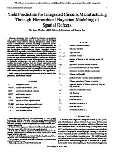
3.1.2 Eight bit binary pattern visualization technique Figure 1 is an example of pattern, trend and relationship between the yields and attributes; CL is the control limit set in percentage by the requirement of process control. A, B and C are the example of attributes continuous values used to relate the relationship with the yield. YD is the point of example where the yield drops below the control limit. The a, b and c are the continuous value from the attributes at the point of yield is below control limit. R1, R2, R3, R4, R5, R6, R7, R8 are the attributes continuous value between the time interval of day or hour. Since engineers plot a chart to visualize and analyze the trend and pattern from multi-variate data bi-variately, the focus is to study the attributes of non-continuous value pattern and trend. The continuous value for each attributes will be visualized with 2 bits values of UP and DOWN pattern from each attributes A, B and C. Every single attributes A, B and C will have the combination of 8 numbers of UP or DOWN pattern for 8 bits visualization case. At YD dotted line on the figure 1, the yield drop down below the control limit, A=a, B = b and C = c; where a, b and c are continuous numbers. The up and down pattern set will be:Ryd (n) = {R1, R2, R3, R4, R5, R6, R7, R8} To obtain UP and DOWN pattern of attribute A:R8 > a then R8 = UP; R7 < R8 then R7 = DOWN; R6 > R7 then R6 = UP; R5 > R6 then R5 = UP; R4 < R5 then R4 = DOWN; R3 > R4 then R3 = UP;

(1)

Fig. 1. Yield and attributes pattern relationships

From the above method, the nominal values UP and DOWN patterns for each attributes A, B and C are:Ryd (A) = {UP, DOWN, UP, UP, DOWN, UP, DOWN, UP} Ryd (B) = {UP, DOWN, DOWN, UP, UP, DOWN, UP, DOWN} Ryd (C) = {DOWN, DOWN, DOWN, DOWN, DOWN, UP, DOWN, DOWN} (2) Since each attributes will have 8 bits or 256 possibilities of pattern, the entire look-up pattern will be defined into a pattern set P:P0={DOWN, DOWN, DOWN, DOWN, DOWN, DOWN, DOWN, DOWN} P1={DOWN, DOWN, DOWN, DOWN, DOWN, DOWN, DOWN, UP} P3={,,..,},P4={..},…...,…..,,, P255= {UP,UP,UP,UP,UP,UP,UP,UP} P={P0,P1,P2,…,P255}

(3)

Finally, we convert the 8 bit binary UP, DOWN pattern generated from each attribute A, B and C into visualized pattern set of 256 elements. The generated instance of case YD indicates that:-

IJCSNS International Journal of Computer Science and Network Security, VOL.9 No.4, April 2009 If R1 (A) = P181 And R1 (B) = P154 And R1 (C) = P4 Then Yield = BAD The example of visualized data instances are tabulated as indicates in Table 1 for the training process with machine learning algorithm. A threshold level was set at a certain level of control limit, for example at yield of 85%. If the yield result is below 85% on a certain day, it will be Table 1: Bad and Good yield visualized pattern dataset Case 1 2 3 4 5 6 7 8 9 10 11 12 13 14 15 16 17 18 19 20

Attribute A P181 P106 P172 P89 P179 P103 P207 P158 P61 P122 P244 P232 P209 P162 P69 P139 P22 P45 P91 P182

Attribute B P154 P52 P201 P147 P38 P76 P153 P50 P101 P202 P148 P40 P81 P162 P69 P138 P20 P41 P83 P166

Attribute C P4 P9 P37 P75 P150 P45 P90 P180 P105 P211 P166 P76 P153 P51 P102 P205 P155 P54 P109 P218

Yield BAD BAD GOOD GOOD GOOD GOOD GOOD GOOD GOOD GOOD GOOD GOOD GOOD GOOD GOOD GOOD GOOD GOOD GOOD GOOD

considered as BAD yield. The BAD yield class is then correlates with the pattern from its attributes trend with 16, 14, 12, 10, 8, 6 or 4 bits value of UP and DOWN pattern. Similarly, if the yield result is above 85% at a certain time, it is also correlates the GOOD yield class with UP and DOWN attributes pattern. In order to obtain the visualized pattern number, the UP and DOWN attributes pattern are converted with the element in the P set of Eq. (3) as shown in Table 1. The process of generating the instances was done by repeating the abovementioned process backward to the time axis.

3.2 Handling Imbalance Datasets Techniques 3.2.1 Random Under-sampling and Over-sampling The implementation of these non-heuristic approaches is very simple. We generated new datasets for training from original dataset by randomly select the instances to under-sampling the majority class instances, oversampling the minority class instances and combination of both under-sampling and over-sampling with specific percentage of sampling process.

127

3.2.2 SMOTE with VDM technique SMOTE technique [15] was proposed to over-sample the minority class by selecting k minority class nearest neighbor instances and producing synthetic instances. Depending on the percentage of over-sampling required, neighbors from the k nearest neighbors are randomly chosen and the synthetic instances were generated by calculating the nearest neighbor numerical dataset with Euclidean distance function. In this study, we are dealing only with nominal value dataset generated by our novel data visualization technique [16]. Therefore, we applied SMOTE oversampling technique with modified Value Distance Metric (VDM) distance function as suggested by [15] to measure and obtain the k nearest neighbor instances. In our case we are using k=5 and to k=1, by selecting 5 and 1 nearest neighbor instances from minority class dataset to generate a synthetic instance. Total numbers of synthetic instances were generated according to the number of over-sampling percentage specified in our experiment procedure. The Value Difference Metric (VDM) distance δ, [19] between two corresponding feature values is defined as follows. (4)

Above equation indicates that, V1 and V2 are the two feature values. C1 is the total number of occurrences of feature value V1, and C1i is the number occurrence of feature value V1 for classes i. C2 is the total number of occurrences of feature value V2, and C2i is the number occurrence of feature value V2 for classes i. k is a constant, normally set to 1. The equation is used to calculate the value differences for each nominal feature in the given set of feature vectors. As in our study, SMOTE-VDM was not used for classification purposes, i is equal to 1 because we only focus on to produce new synthetic instances from minority class instances. To generate new minority class instances, [15] proposed to create new set instances values by taking the majority vote of the feature vector in consideration from its k nearest neighbors. Below shows an example of creating a synthetic instance by majority vote proposed. Let F1 = P234 P1112 P3345 P975 P335 be the instance under consideration and let its 5 nearest neighbors as; F2 = P675 P678 F3 = P234 P789 F4 = P776 P456 F5 = P1234 P3567 F6 = P234 P1112

P2341 P1234 P2334 P2242 P3345 P2334 P3456 P987 P567 P1112 P3345 P453 P3345 P765 P777

128

IJCSNS International Journal of Computer Science and Network Security, VOL.9 No.4, April 2009

The application of SMOTE-Nominal would create the following instance: FS = P234 P1112 P3345 P3345 P2334 However, we are dealing with poly-nominal data not with normal nominal value. The poly-nominal data which was visualized by 12 bit number creates 4096 possibility of nominal value for each attribute. Hence, there is a possibility that the majority vote technique to generate the synthetic value may not be feasible. This potentially was due to the high possibilities that there will be no redundant pattern number available for voting from the selected k nearest neighbors. Thus, we included an option in the VDM distance function by calculating the average of those 5 nearest neighbor selected in the instances attributes by converting the pattern number into integer and then transform the calculated average number back to pattern number. Anyhow, in the case of k equal to 1, the synthetic instances were generated directly from the selected nearest neighbor instances. The threshold for VDM distance value in this study is 0.1. The VDM distance algorithm generates k nearest instance if the distance between two feature vectors which was randomly selected is less than 0.1. Zero is the ideal distance for similarity feature vector value but it is computationally expensive.

3.2.3 SMOTE with K* Entropy SMOTE technique [15] was proposed to over-sample the minority class by selecting k minority class nearest neighbor instances to produce synthetic instances. Depending on the percentage of over-sampling required, neighbors from the k nearest neighbors are randomly chosen and the synthetic instances were generated by calculating the nearest neighbor numerical dataset with Euclidean distance function. We integrates the K* entropy based similarity distance function. Total numbers of synthetic instances were generated according to the number of over-sampling percentage required in our experiment.

3.2.4 SMOTE and Random Under-sampling This approach was applied in our previous study [22] where Value Difference Metric (VDM) was implemented as similarity distance function for SMOTE. Random under-sampling sampled from majority class instances until the instances numbers exactly balance up with SMOTE percentage. The result from this approach will

compare the significant of K* entropy based distance function with VDM.

3.2.5 One Sided Selection Under-sampling As suggested by [26], we applied the approach to verify the importance of balance distribution between majority and minority instances in order to produce robust classifiers. In this paper, we applied ONESS approach by under-sampling the majority instances with CNN and CNN+Tomek Links. The result from those algorithms verifies the relationships of redundant and borderline majority instances on our visualized data pattern on minority instances.

3.2.6 SMOTE and CNN+Tomek Under-sampling This approach applied K* bases entropy similarity distance function on the SMOTE and CNN+Tomek undersampling. The distribution of the minority and majority were made exactly balanced by limit the CNN+Tomek under-sampling process until it reach the SMOTE instances percentage. The lowest percentage of SMOTE allow CNN+Tomek under-sampling to process further deeper compare to the higher percentage of SMOTE. Since the Tomek process will push majority instances further lower than the number of available minority instances, this approach is actually equivalent to perform under-sampling with CNN algorithm alone without Tomek links.

3.2.7 SMOTE and SMaRT (CNN+Tomek) Our proposed SMaRT technique applied the undersampling with CNN+Tomek algorithm until it reaches to the end of the process. The number of majority instances left after the process is smaller compared with minority class instances. Thus, SMaRT used SMOTE algorithm and K* entropy similarity distance function to generate the synthetic majority instances until it is balanced with minority number of instances generated by specified percentage of SMOTE.

3.2.8 SMOTE and SMaRT (CNN) This approach is similar with aforementioned above, except that we only implemented SMaRT with CNN alone without the Tomek Links algorithm. The result between these 2 approaches indicates the relationships of redundant and borderline/noisy instances with our visualized data sets whether they carries significant differences. Once the CNN process ended, the majority instances populated are bigger from minority instances. When SMOTE at smaller percentage, CNN generates the majority instances slightly bigger and SMaRT will not

IJCSNS International Journal of Computer Science and Network Security, VOL.9 No.4, April 2009

generates synthetic majority instances. At the higher SMOTE percentage, SMaRT instances will get into the distribution.

3.3 F-Score Performance Measure We used F-Score to measure the overall performance of the sampled datasets studied. F-measure is a harmonic mean between recall and precision defined as:-

129

greedy type learning algorithm, we only compare the prediction test between raw data and 8 bit visualized datasets with IBk, K* and LWL. We also visualized the raw dataset into 4,6,8,12,14 and 16 bits training and test datasets, and then trained them with the IBk, K* and LWL algorithms. This experiment purpose is to find for the best bit number for the visualization technique and to select a best classifier from those 3 algorithms.

4.1.3 Result analysis (5)

The F-measure becomes zero if either R or P is zero and it will become 1 when both R and P are 1. R is recall and P is precision. Recall and precision are define as:-

Training result with the raw dataset in Table 2 shows that IBk and J48 were the best performers where the others algorithm had problem with the bad yield (minority) class prediction and recall at the average of 70.2%. With IBk and J48, the average class precision is 95.2% and 94% and the average class recall is 92.6% and 92.6%. The result shows that the selected datasets attributes indicates the strong relationships with the manufacturing yield.

(6) Table 2: Raw dataset training result

(7) CP is the number of instances that are correctly predicted as positive and TP is the number of actual positive instances, where PP is total number instances predicted as positive.

4. Study results 4.1 Visualized datasets 4.1.2 Experimental procedure The data fields used for the study were ID, Total Yield Percentage, RankA, G-NG, R-NG, Ring, Hit, MP1, MP2, MP3, Q3MP3 and Yield class instance. The visualized data into binary bits pattern number was generated from the same raw data. Prediction test was done with dataset which was visualized into binary bits pattern from the same test raw data. In this study we were using Decision Stump, J48, Naïve Bayes, IBk, K* and LWL algorithm for the learning process with confusion matrix and stratified 10-fold cross validation. Firstly, we performed the training process with the raw data to clarify the attributes relationships strength amongst the class instance and to seek for the best algorithm. We then trained the 8 bit visualized dataset to check for prediction feasibility, performance and the best algorithm. Since the results shows that lazy learning algorithm (instance base learner) perform the best compared to the

Weka Decision Stump class true preci GOO true sion D BAD pred. 55.3 BAD 316 255 4% pred. 95.6 GOOD 613 13490 5% class 34.02 98.14 recall % % Weka IBk class true preci GOO true sion D BAD pred. 91.2 BAD 796 76 8% pred. 99.0 GOOD 133 13669 4% class 85.68 99.45 recall % % NaïveBayes true class true GOO preci BAD D sion pred. 65.0 BAD 809 435 3% pred. 99.1 GOOD 120 13310 1% class 87.08 96.84 recall % %

Weka J48 class true preci GO true sion OD BAD 88.8 799 100 8% 1364 99.0 130 5 6% 86.01 99.2 % 7% Weka KStar class true preci GO true sion OD BAD 92.3 276 23 1% 1372 95.4 653 2 6% 29.71 99.8 % 3% Weka LWL true class true GO preci BAD OD sion 54.8 336 277 1% 1346 95.7 593 8 8% 36.17 97.9 % 8%

Anyhow, Table 3 shows that the decision tree classifier Decision Stump and J48 failed to classify the training data with the 8 bit visualized dataset. IBk, K* and LWL algorithm training result performs at acceptable performance where the average class precision for K* is

IJCSNS International Journal of Computer Science and Network Security, VOL.9 No.4, April 2009

130

97.1%, IBk is 75.7% and LWL is 95.3%. The average class recall for K* is 62.4%, IBk is 63% and LWL is 55.8%. The results from the experiment indicates that the proposed technique of the binary 8 bits visualized dataset is feasible to be considered for the “one step ahead” future prediction of the yield. The prediction test with raw dataset in Table 4 shows that IBk is the best learner algorithm to predict the raw data yield outcome with the average of 99% for class 76.7%.

precision and recall, where K* average class precision and recall is 85.4% and LWL is 84.5%. On the other hand, 8 bit visualized datasets test result in table 5 shows that both IBk and K* giving good result where the average class precision and class recall is 95.9%. LWL produce the worst result where the average class precision and recall is Table 5: 8 Bit visualized prediction test result Weka IBK

Table 3: 8 Bit visualized datasets training result Weka Decision Stump

. pred. BAD pred. GOOD class recall

pred. BAD pred. GOOD class recall

pred. BAD pred. GOOD class recall

true BAD

true GOOD

0

0

785 12408 0.00 100.00 % % Weka IBk true BAD

true GOOD

215

170

570 12238 27.3 9% 98.63% NaïveBayes true BAD

true GOOD

146

240

639 18.6 0%

12168

class preci sion ? 94.0 5%

class preci sion 55.8 4% 95.5 5%

class preci sion 37.8 2% 95.0 1%

98.07%

Weka J48 class true preci GO true sion OD BAD 0

0 1240 785 8 100. 0.00% 00% Weka KStar true GO true OD BAD 196

pred. GOOD pred. BAD class recall

? 94.0 5%

pred. GOOD pred. BAD class recall

class preci sion 85.9 6% 95.4 6%

32 1237 589 6 99.7 24.97% 4% Weka LWL class true preci GO true sion OD BAD 95.8 92 4 3% 1240 94.7 693 4 1% 99.9 11.72% 7%

pred. GOOD pred. BAD class recall

pred. GOOD pred. BAD class recall pred. GOOD pred. BAD class recall pred. GOOD pred. BAD class recall

true BAD

class precision

203

1

99.51%

0

28

100.00%

96.55% Weka KStar 15

93.12%

0

14

100.00%

100.00%

8

10

203

48.28% Weka LWL

12

14

179

1

99.44%

24

28

53.85%

88.18%

96.55%

185

4

97.88%

0

24

100.00%

100.00%

85.71% Weka KStar

185

4

97.88%

0

24

100.00%

100.00%

85.71% Weka LWL

185

23

88.94%

0

5

100.00%

100.00%

17.86%

16

Weka KStar

Weka LWL

Class

class recall

class preci sion

class recall

class precisi on

class recal l

class preci sion

BAD

0.34

0.47

0.12

0.68

0.00

?

GOOD

0.97

0.96

1.00

0.94

1.00

0.94

BAD

0.31

0.51

0.20

0.73

0.01

0.78

GOOD

0.98

0.96

1.00

0.95

1.00

0.94

BAD

0.27

0.56

0.25

0.86

0.12

0.96

GOOD

0.99

0.96

1.00

0.95

1.00

0.95

BAD

0.27

0.50

0.26

0.95

0.24

0.80

GOOD

0.98

0.96

1.00

0.96

1.00

0.95

BAD

0.29

0.68

0.27

0.98

0.28

0.57

GOOD

0.99

0.96

1.00

0.96

0.99

0.96

BAD

0.27

0.65

0.26

0.97

0.28

0.58

GOOD

0.99

0.96

1.00

0.96

0.99

0.96

BAD

0.30

0.62

0.28

0.92

0.29

0.68

GOOD

0.99

0.96

1.00

0.96

0.99

0.96

Bit

6

100.00%

class precision

Weka IBk

4

true GOOD

true BAD

Table 6: Multiple bit value visualized training result

Table 4: Raw dataset prediction test result Weka IBK

true GOOD

IJCSNS International Journal of Computer Science and Network Security, VOL.9 No.4, April 2009

Training with multiple bit value visualized datasets results in table 6 shows that the class precision and class recall improving with the higher number of bits value. K* is the best performer and 12 bit visualized pattern is the best bits value where the average class precision is 96.6% and average class recall is 63.6%. IBk result is better with average class precision of 81.97% and average class recall is 63.9% compare to LWL with an average class precision of 76.3% and class recall of 63.4%. However, even though K* produced the best prediction accuracy result compare to the other algorithm, the class recall for the BAD yield (minority class) is still not achieving significant improvement, it was not able to surplus 30% even with higher bit visualized datasets. 4.2 Handling imbalance datasets 4.2.1 Experimental Procedure We were using the same data from our previous study [16]. The data fields used for the study are ID, Total Yield Percentage, RankA, G-NG, R-NG, Ring, Hit, MP1, MP2, MP3, Q3MP3 and Yield class instance. 12 bit visualized training dataset was used as the original dataset to generate the new training datasets. For plain random under-sampling training dataset, they were generated by 30%, 40%, 50%, 60%, 70% and 80% from the original majority class dataset. We created 50%, 100%, 150%, 200%, 250% and 300% training datasets for random oversampling as well as SMOTE oversampling from the original minority class dataset. As for the combination sampling of random oversampling + undersampling and SMOTE + random under-sampling datasets, the datasets were created by over-sampling the original dataset minority class by 50%, 100%, 150%, 200%, 250% and 300% and then randomly under-sampling the original majority class instances until the distribution will be exactly balanced with over-sampled instances. Combination sampling of SMOTE+Random_Undersampling, SMOTE+SMaRT (CNN+Tomek), SMOTE+SMaRT (CNN), SMOTE+CNN Under-sampling datasets were created by over-sampling the original dataset minority class by 50%, 100%, 150%, 200%, 250% and 300% and then under-sampling or SMaRTing the original majority class instances until it is reached to the exactly balanced distribution with over-sampled instances. We also generate ONESS datasets by under-sampled the majority instances with [8] CNN (Condense Nearest Neighbor)+Tomek Links and CNN to verify the importance of the exact balance distribution between majority and minority instances for our visualized data sets.

131

Training datasets were trained with K* algorithm as recommended [16] for the learning process with confusion matrix and stratified 10-fold cross validation configured. The classifiers generated from the training data were then being tested with a test dataset from the same batch of training dataset. The classifiers once again been tested with different batches test dataset to test the robustness of the generated classifiers. The result of the training and prediction test are compared to verify the effectiveness of the integration of VDM and K* entropy base similarity distance function and also the improvement of the F-Score measure on the robustness of the generated classifiers. 4.2 Result analysis Training result in table 7 shows that random undersampling the majority class instance did not giving significant improvement to the class recall and precision as compared to the original dataset. Over-sampling results indicates that by over-sampling the minority class instances randomly, the class recall increases proportionally with Table 7: Training result for under-sampling, over-sampling and its combination Data Sets

Performance R

P

F

0.273

0.976

0.427

30%

0.273

0.990

0.428

40%

0.265

0.975

0.417

50%

0.274

0.922

0.422

60%

0.281

0.945

0.434

70%

0.257

0.887

0.399

80%

0.282

0.777

0.414

50%

0.684

0.991

0.810

100%

0.827

0.991

0.902

150%

0.914

0.989

0.950

200%

0.955

0.984

0.969

250%

0.975

0.981

0.978

300%

0.981

0.976

0.978

50%

0.826

0.739

0.780

100%

0.907

0.791

0.845

150%

0.957

0.975

0.966

200%

0.975

0.807

0.883

250%

0.986

0.815

0.892

300%

0.993

0.829

0.903

Original data set Undersampling

Oversampling

Over+Undersampling

sampling percentage without significantly affecting the

IJCSNS International Journal of Computer Science and Network Security, VOL.9 No.4, April 2009

132

class precision. Hence, the F value shows significant improvement proportionally with higher number of the minority class instance oversampling. The combination of balance random over and under-sampling result shows that the class recall increases proportionally with the number of sample but inconsistently affecting the precision. Even though the F value shows significant improvement compare to the original data set, over-sampling minority class instances produce the best result between these three sampling method. Table 8: Training result of SMOTE-VDM with k=5 and combination with under-sampling Data Sets

Performance

Table 8 shows the training result of proposed technique SMOTE+VDM with nearest neighbor k=5. The result indicates that the sampling method was not able to improve the class recall. The result was even worse than the original datasets training outcome. Combination SMOTE+VDM with k=5 and under-sampling shows better performance. However, the result was still not able to overwhelm the plain over-sample and over + undersampling method outcome. Anyhow, Table 9 shows that the SMOTE+VDM with k=1 result performs better than k=5 for both with or without under-sampling the majority class instances. The SMOTE+VDM and k=1, with and without under-sampling both showed better performance from each other at difference sampling percentage. However, the result still underperforms the simple plain random over-sampling method.

R

P

F

50%

0.193

0.964

0.322

100%

0.146

0.947

0.252

150%

0.117

0.926

0.208

200%

0.137

0.921

0.239

250%

0.165

0.934

0.280

300% SMOTE+VDM k=5 and Undersampling

0.187

0.913

0.310

50%

0.539

0.741

0.624

Original data set

0.920

1.000

0.958

100%

0.612

0.816

0.700

Undersampling 60%

0.960

1.000

0.980

150%

0.656

0.851

0.741

Oversampling 300%

1.000

1.000

1.000

200%

0.627

0.828

0.714

Over+Undersampling 300%

1.000

0.481

0.649

250%

0.592

0.871

0.705

0.880

1.000

0.936

300%

0.731

0.897

0.805

SMOTE+VDM, k=1 300% SMOTE+VDM,k=1 Undersampling 250%

1.000

0.532

0.694

0.840

1.000

0.913

0.960

0.686

0.800

SMOTE-VDM k=5

Table 10: Prediction test result with same batch test data Data Sets

Performance R

SMOTE+VDM k=5 50% SMOTE+VDM,k=5 Undersampling 300%

P

F

Table 9: Training result of SMOTE-VDM with k=1 and combination with under-sampling Data Sets

Table 11: Prediction test result with difference batch test data

Performance R

P

F

Data Sets

SMOTE+VDM k=1 50%

0.211

0.967

0.346

100%

0.438

0.992

0.608

150%

0.729

0.965

0.831

200%

0.663

0.977

0.790

250%

0.822

0.957

0.884

300% SMOTE+VDM k=1and Undersampling

0.846

0.958

0.898

50%

0.798

0.790

0.794

100%

0.881

0.773

0.823

150%

0.895

0.835

0.864

200%

0.962

0.731

0.831

250%

0.934

0.823

0.875

300%

0.963

0.774

0.858

Performance R

P

F

0.000

0.000

0.000

Undersampling 60%

0.000

0.000

0.000

Oversampling 300%

0.000

0.000

0.000

Original data set

Over+Undersampling 300%

0.571

0.281

0.376

SMOTE+VDM k=1 300% SMOTE+VDM k=1 Undersampling 250%

0.071

1.000

0.133

0.500

0.286

0.364

0.000

0.000

0.000

0.536

0.333

0.411

SMOTE+VDM k=5 50% SMOTE+VDM k=5 Undersampling 300%

IJCSNS International Journal of Computer Science and Network Security, VOL.9 No.4, April 2009

Table 10, 11 and 12 show the result of the prediction test with the classifiers generated by the training data. The results were based from the best performer classifiers selected from each sampling method. Table 10 indicates the prediction test with the testing dataset from the same batch of training data. The result shows that over-sampling performs the best result while the combination type of sampling method did not really perform better as compared to the other single type sampling method. Both Table 11 and 12 results were tested with data from different batches. The results indicated that sampling method that uses combination of over-sampling and under-sampling is capable to perform the prediction compared to the single type sampling methods which were totally failed. SMOTE+VDM and under-sampling method shows better result than the combined plain over-sampling and under-sampling method. Table 13, 14, 15 and 16 show that SMOTE+Random Under-sampling with K* based entropy similarity distance function performs better compared to the integration of SMOTE with VDM distance function. The results in Table 13 also indicates that SMOTE+SMaRT training result significantly performs better than the other double sided sampling techniques and also outperform the ONESS Over-sampling method resulted in our previous study [22]. While significantly improving the training result, SMOTE+SMaRT remain its robustness, and also performs better from previous study [22], a result which is in contrast behavior compared to over-sampling technique. Comparing SMOTE+SMaRT with CNN and CNN+Tomek, Table 14 and 16 indicates that SMOTE+SMaRT(CNN) outperforms SMOTE+SMaRT(CNN+Tomek), while Table 13 and 15 show a contrast result. Table 13, 15 and 16 also show that SMOTE+SMaRT(CNN) perform better with the increase of SMOTE percentage (SMaRT instances distribution also increased).

The implementation of CNN alone compared with CNN+Tomek did not indicate significant different, except that the Table 14 shows the implementation of CNN algorithm performs significantly better especially with ONESS approach. Table 14 also indicates that the F-Score with CNN decrease when the SMOTE percentage increase. This shows that, CNN at the lower percentage of SMOTE causing the majority instances distribution slightly outnumbered the minority instances (but the SMaRT with CNN is better than under-sampling with CNN). However, the trend was not true in Table 13, 15 and 16. Table 13: Classifiers training result of bad yield class instances Performance R

Original data set

0.000

P 0.000

F

0.79

0.879

0.30

0.58

0.399

50%

0.83

0.77

0.798

100%

0.91

0.79

0.847

150%

0.95

0.80

0.869

200%

0.97

0.80

0.880

250%

0.98

0.81

0.891

300%

0.99

0.82

0.897

50%

0.78

0.67

0.720

100%

0.88

0.64

0.745

150%

0.97

0.61

0.751

200%

0.98

0.64

0.771

250%

0.99

0.65

0.788

300%

0.99

0.68

0.807

50%

0.84

1.00

0.914

100%

0.91

1.00

0.955

150%

0.96

1.00

0.979

200%

0.98

1.00

0.990

250%

0.99

1.00

0.993

300%

1.00

1.00

0.998

Under-sampling CNN Under-sampling SMOTE+Random Under-sampling

SMOTE+CNN Under-sampling

Performance R

P

0.99

Tomek+CNN

SMOTE+SMaRT (TOMEK+CNN)

Table 12: Prediction test result with another difference batch test data Data Sets

133

F 0.000

Undersampling 60%

0.000

0.000

0.000

Oversampling 300%

0.000

0.000

0.000

Over+Undersampling 300%

0.346

0.180

0.237

SMOTE+VDM k=1 300% SMOTE+VDM k=1 Undersampling 250%

0.000

0.000

0.000

0.385

0.196

0.260

SMOTE-VDM k=5 50% SMOTE-VDM Undersampling 300%

0.000

0.000

0.000

0.346

0.220

0.269

k=5

SMOTE+SMaRT(CNN) 50%

0.74

0.66

0.698

100%

0.88

0.66

0.755

150%

0.95

0.69

0.798

200%

0.98

0.76

0.855

250%

0.99

0.83

0.901

300%

0.99

0.87

0.924

IJCSNS International Journal of Computer Science and Network Security, VOL.9 No.4, April 2009

134

For the ONESS approach, even though CNN undersampling shows significant better result (Table 14), but it did not produce robust classifier as indicated in Table 13, 15 and 16. CNN+Tomek under-sampling produce quite a robust classifier accepts for the result indicates in Table 14, where the result is at the lowest level compared to the other approaches. We also can see that CNN+Tomek under-sampling is producing the best performance for class recall in overall result but lower in class precision, while Table 14: Classifiers same batch data test result of bad yield class instances

the other approaches sacrificing class recall to raise up the class precision in order to improve the F-Score. A result of ONESS approach shows that, it is crucial to remove the borderline and noisy instances in order to produce a robust classifier.

Table 15: Classifiers different badge data test result of bad yield class instances

Performance R Tomek+CNN

Performance

P

F

1.00

0.13

0.230

0.92

0.82

0.868

Under-sampling

Tomek+CNN

R

P

F

1.00

0.26

0.415

0.07

0.22

0.108

Under-sampling

CNN Under-sampling SMOTE+Random Under-sampling

CNN Under-sampling SMOTE+Random Under-sampling

50%

0.96

0.38

0.539

50%

0.61

0.29

0.391

100%

0.96

0.42

0.585

100%

0.64

0.30

0.405

150%

0.96

0.47

0.632

150%

0.43

0.24

0.304

200%

1.00

0.39

0.562

200%

0.57

0.30

0.395

250%

1.00

0.43

0.602

250%

0.39

0.20

0.265

300%

0.92

0.42

0.575

300%

0.64

0.33

0.434

SMOTE+CNN Under-sampling

SMOTE+CNN Under-sampling 50%

0.96

0.57

0.716

50%

0.71

0.33

0.449

100%

1.00

0.52

0.685

100%

0.54

0.27

0.361

150%

0.96

0.25

0.400

150%

0.75

0.30

0.424

200%

0.96

0.22

0.356

200%

0.79

0.30

0.436

250%

1.00

0.20

0.333

250%

0.86

0.29

0.432

300%

1.00

0.19

0.325

300%

0.82

0.29

0.426

SMOTE+SMaRT (TOMEK+CNN)

SMOTE+SMaRT (TOMEK+CNN) 50%

0.96

0.32

0.485

50%

0.71

0.32

0.440

100%

1.00

0.32

0.481

100%

0.68

0.29

0.409

150%

0.96

0.31

0.471

150%

0.71

0.32

0.440

200%

0.96

0.30

0.462

200%

0.75

0.35

0.477

250%

1.00

0.32

0.481

250%

0.71

0.29

0.412

300%

0.96

0.29

0.444

300%

0.68

0.32

0.432

SMOTE+SMaRT (CNN)

SMOTE+SMaRT (CNN) 50%

0.88

0.79

0.830

50%

0.29

0.31

0.296

100%

0.96

0.34

0.505

100%

0.54

0.32

0.400

150%

1.00

0.46

0.633

150%

0.61

0.29

0.391

200%

0.96

0.43

0.593

200%

0.54

0.26

0.353

250%

1.00

0.34

0.510

250%

0.61

0.29

0.391

300%

1.00

0.35

0.521

300%

0.61

0.33

0.430

IJCSNS International Journal of Computer Science and Network Security, VOL.9 No.4, April 2009

Table 16: Classifiers different badge data test result of bad yield class instances Performance

Tomek+CNN

R

P

F

1.00

0.22

0.361

0.04

0.20

0.065

Under-sampling CNN Under-sampling SMOTE+Random Under-sampling 50%

0.54

0.21

0.301

100%

0.35

0.15

0.209

150%

0.42

0.21

0.278

200%

0.46

0.20

0.279

250%

0.46

0.24

0.320

300%

0.31

0.16

0.211

SMOTE+CNN Under-sampling 50%

0.58

0.21

0.303

100%

0.58

0.25

0.345

150%

0.77

0.25

0.377

200%

0.88

0.26

0.407

250%

0.77

0.24

0.364

300%

0.92

0.26

0.410

50%

0.58

0.21

0.306

100%

0.62

0.23

0.330

150%

0.50

0.20

0.289

200%

0.58

0.22

0.323

250%

0.62

0.23

0.333

300%

0.65

0.22

0.330

0.255

SMOTE+SMaRT (TOMEK+CNN)

SMOTE+SMaRT (CNN) 50%

0.27

0.24

100%

0.38

0.21

0.270

150%

0.62

0.25

0.352

200%

0.42

0.20

0.268

250%

0.42

0.20

0.272

300%

0.46

0.23

0.304

5. Conclusion and Further Research The combination of K* learning algorithm with 12 bit pattern visualized datasets produces the best class precision and recall result. This indicates that the method of visualizing the pattern with the proposed binary bit pattern method is feasible to be used with machine

135

learning algorithm in order to predict future manufacturing yield. Since most of the temporal data learning performs batch by batch basis, this data visualization technique can be used for automatic data exploration to learn the pattern and trend and then updating them from time to time into a learning repertory engine. The Bad yield (minority instances) class recall performance issue due to the imbalance datasets (due to the nature of manufacturing process) can be improved by identifying the pattern and trend that has strong relationships with the bad (minority) and good (majority) class instances. Combination with other technique such as [15] SMOTE (Synthetic Minority Over Sampling Technique), conventional over sampling minority class or under sampling majority class can be applied to further improve the Bad yield (minority) class recall drawback. Handling the imbalance datasets merely by undersampling alone was not able to give any significant improvement; but in contrast, the over-sampling method has produced the best performance. Furthermore, oversampling result outperformed our proposed SMOTEVDM and SMOTE-VDM + under-sampling. However, the prediction test result indicates that, the combination of under-sampling and over-sampling was able to deal wider range of test datasets. As such, SMOTE+VDM and undersampling produced the most robust classifier performance which is capable to perform better with all those three different batches of prediction test data. In comparison of the similarity distance function, K* based entropy similarity distance function perform better than VDM for the visualized data sets. Our suggested approach of SMOTE+SMaRT also improved the classification robustness compared to the previous approaches. Well balanced number of instances in the datasets produces robust classifier but further improvement on the performance is required. However, the exact balance of minority and majority classes are not the main concern to handle the imbalance data sets. The most important matter to focus is the balance distribution of the relevant information carried by each class instances. This is because the random under-sampling has the potential of information loss which affecting the class precision, whilst over-sampling method will improve the class recall with mild impact to the precision but carry the risk of overfitting. Hence, we conclude that over-sampling with appropriate synthetic minority instance is important to improve the class recall with minimum impact to overfitting. On the other hand, because under-sampling causes the information loss and reducing the class precision, an approach such as SMaRT selectively sampling out the majority class instances is also important for future study. A study to improve the class precision without sacrificing

136

IJCSNS International Journal of Computer Science and Network Security, VOL.9 No.4, April 2009

class recall of the minority instances is very crucial in order to further extend the classifiers robustness and predicting performance. Hence, a method on how to handle with the redundant, borderline, noisy instances and also to effectively generate synthetic instances (both for over-sampling and under-sampling) should be the main focus. Another approach that can be considered for the improvement is to select the best trained classifiers performer at respective area and combine them into one. Acknowledgement This research is funded by FRGS (Fundamental Research Grant Scheme) from Malaysia Higher Ministry of Education for Intelligent Predictive Maintenance System for Hard-Disk Media Manufacturing Using Data Mining Approach. References [1] P. W. Tse, “Maintenance practices in Hong Kong and the use of the intelligent scheduler”. Journal of Quality in Maintenance Engineering, (2002). 8(4), 369-380 [2] W.M. Gibbons, M. Ranta, T.M. Scott, M. Mantyla, “Information Management and Process Improvement Using Data Mining Techniques”, Intelligent Problem Solving. Methodologies and Approaches: 13th International Conference on Industrial and Engineering Applications of Artificial Intelligence and Expert Systems, IEA/AIE 2000, New Orleans, Louisiana, USA, June 2000. Proceedings (pp 93-98). Berlin / Heidelberg: Springer. [3] M. Gardner and J. Bieker, “Data Mining Solves Tough Semiconductor Manufacturing Problems”, Conference on Knowledge Discovery in Data Proceedings of the sixth ACM SIGKDD international conference on Knowledge discovery and data mining, (2000). (pp 376 - 383). New York, NY, USA: ACM Press. [4] Kittler and W. Wang, “Data Mining for Yield Improvements”, Proc. Intl Conf. on Modeling and Analysis of Semiconductor Manufacturing, Tempe, USA. May, 2000. [5] F. Mieno, T. Sato, Y. Shibuya, K. Odagiri, H. Tsuda and R. Take. “Yield improvement using data mining system”, Semiconductor Manufacturing Conference Proceedings, 1999 IEEE International Symposium (pp 391-394). Santa Clara, CA, USA. [6] Braha, D., Elovici, Y., & Last, M. (2007). “Theory of actionable data mining with application to semiconductor manufacturing control”. International Journal of Production Research, 45(13), 3059–3084. [7] I. H. Witten and E. Frank, “Data Mining: Practical Machine Learning Tools and Techniques with Java Implementations”, Morgan Kaufmann, (1999) San Francisco, CA, USA. [8] I. Mierswa and M. Wurst and R. Klinkenberg, M. Scholz and T. Euler. “YALE: Rapid Prototyping for Complex Data Mining Tasks”, in Proceedings of the 12th ACM SIGKDD International Conference on Knowledge Discovery and Data Mining (KDD-06), 2006.

[9] K. Ron. “Data Mining and Visualization” In: Sixth Annual Symposium on frontiers of Engineering, National Academy Press, D. C., 2001, p. 30 40. [10] A. K. Daniel. “Information Visualization and Visual Data Mining”. IEEE Transactions on Visualization and Computer Graphics, Vol. 8, No. 1, January-March 2002 [11] S. A. Jes´us, J. F. Francisco. “Visual Data Mining”. J.UCS Special Issue Journal of Universal Computer Science. vol. 11, no. 11 (2005), 1749-1751 [12] S. Jörn, S. Mike, A.K. Daniel. “Information Visualization.” 6, 75 – 88, 2007 Palgrave Macmillan Ltd. [13] T. T. Soon, Z. Ke, M. T. Shih, L. M. Kwan, S. F. Wu. “Combining Visual and Automated Data Mining for Near Real Time Anomaly Detection and Analysis in BGP”. VizSEC/DMSEC’04, October 29, 2004, Washington, DC, USA. [14] U. Demšar. “Data mining of geospatial data: combining visual and automatic methods”. Doctoral thesis in Geoinformatics Department of Urban Planning and Environment School of Architecture and the Built Environment Royal Institute of Technology (KTH) Stockholm, April 2006. [15] V. C. Nitesh, W. B. Kevin, O. H. Lawrence, W. P. Kegelmeyer. “SMOTE: Synthetic Minority Over-sampling Technique”. Journal of Artificial Intelligence Research 16 (2002) 321–357 [16] Megat Norulazmi Megat Mohamed Noor, Shaidah Jusoh, “Visualizing the Yield Pattern Outcome for Automatic Data Exploration”, ams, pp. 404-409, 2008 Second Asia International Conference on Modeling Simulation, 2008. [17] Y. Kihoon, K. Stephen. “A data reduction approach for resolving the imbalanced data issue in functional genomics” Journal of Neural Computing & Applications Volume 16, Number 3 / May, 2007 Pages 295-306 Springer London. [18] M. G. Karagiannopoulos, D. S. Anyfantis, S. B. Kotsiantis and P. E. Pintelas. “Local Cost Sensitive Learning for Handling Imbalanced Data Sets Control & Automation”, 2007. MED '07. Mediterranean Conference on 27-29 June 2007 page(s): 1-6 Athens, Greece. [19] R. P. Terry and E. Peter. “Implicit Feature selection with the value difference metric”, Proceedings of the 13th European Conference on Artificial Intelligence, ECAI-98, John Wiley & Sons, New York, NY, 1998, pp. 450-454. [20] D. Joshi. (2004). Applying the wrapper approach for auto discovery of under-sampling and over-sampling percentages on skewed datasets, M.Sc. Thesis, Univ. South Florida, Tampa [Online]. pp. 1–77. Available: http://etd.fcla.edu/SF/SFE0000491/Thesis-AjayJoshi.pdf [21] G. E. A. P. A. Batista, A. L. Bazan, and M. C. Monard. “Balancing Training Data for Automated Annotation of Keywords: a Case Study”. In Proceedings of the Second Brazilian Workshop on Bioinformatics, pages 35–43, 2003. [22] Megat Norulazmi Megat Mohamed Noor and Shaidah Jusoh, “Handling Imbalance Visualized Pattern Dataset for Yield Prediction” 3rd International Symposium on Information Technology 2008, 26 -29 August, Page(s):1 - 6 [23] G. C. John and E. T. Leonard “{K}*: an instance-based learner using an entropic distance measure”, Proc.12th

IJCSNS International Journal of Computer Science and Network Security, VOL.9 No.4, April 2009

[24]

[25] [26]

[27]

International Conference on Machine Learning, Morgan Kaufmann 108—114 1995. M. Kubat and S. Matwin. “Addressing the Curse of Imbalanced Training Sets: One-Sided Selection”, Proc.14th Int’l Conf. on Machine Learning (ICML’97), pp.179-186, Nashville, USA (1997). I. Tomek. “Two Modifications of CNN”, IEEE Trans. Systems, Man and Cybernetics, SMC.6, pp. 769-772 (1976). Y. Kamei, A. Monden, S. Matsumoto, T. Kakimoto, K .Matsumoto. “The Effects of Over and Under Sampling on Fault-prone Module Detection”, Empirical Software Engineering and Measurement, 2007. ESEM 2007. First International Symposium on Volume, Issue, 20-21 Sept. 2007 Page(s):196 – 204. Megat Norulazmi Megat Mohamed Noor and Shaidah Jusoh, “Improving F-Score of the Imbalance Visualized Pattern Dataset for Yield Prediction Robustness”, 21st International CODATA Conference, Kyiv, Ukraine, 5-8 October 2008, page 203-211

Megat Norulazmi Megat Mohamed Noor is a PhD in IT candidate of Universiti Utara Malaysia. He received the B.S degrees in Electronic Engineering from Kagoshima University, Japan in 1994 and Master of IT from Open University Malaysia on 2007. He was a Senior Engineer in hard disk media industry for about 10 years.

Shaidah Jusoh is currently a senior lecturer at Graduate Dept. of Computer Science, College of Arts and Sciences at Universiti Utara Malaysia. She received her PhD degree in Engineering System & Computing, 2005, and MSc degree in Computer Science, 1998 from University of Guelph, Canada. She has published 40 articles in refereed international journals and proceedings. Her research interests include text mining, data mining, robotics, information extraction, databases, natural language processing and fuzzy approach applications.

137