Visualizing the Results of Field Testing Brian Chan, Ying Zou
Ahmed E. Hassan
Anand Sinha
Dept. of Elec. and Comp. Engineering Queen’s University Kingston, Ontario, Canada {2byc, ying.zou}@queensu.ca
School of Computing Queen’s University Kingston, Ontario, Canada
[email protected]
Handheld Software Research in Motion (RIM) Waterloo, Ontario, Canada
[email protected]
Abstract— Field testing of software is necessary to find potential user problems before market deployment. The large number of users involved in field testing along with the variety of problems reported by them increases the complexity of managing the field testing process. However, most field testing processes are monitored using ad-hoc techniques and simple metrics (e.g., the number of reported problems). Deeper analysis and tracking of field testing results is needed. This paper introduces visualization techniques which provide a global view of the field testing results. The techniques focus on the relation between users and their reported problems. The visualizations help identify general patterns to locate the problems. For example, the technique identifies groups of users with similar problem profiles. Such knowledge helps reduce the number of needed users since we can pick representative users. We demonstrate our proposed techniques using the field testing results for four releases of a large scale enterprise application used by millions of users worldwide. Keywords- User Logs; Visualization; Pattern Identification; Automation
I.
INTRODUCTION
Software must endure rigorous field testing before market deployment. Field testing helps uncover problems due to unexpected user behaviors and unforeseen usage patterns in a natural setting. Instrumented versions of the application are used during field testing. These versions enable the collection of field data in real-time without developer interference. A problem report is sent and stored in a central repository when an unexpected situation occurs. Common information in the report includes error messages and call stacks for a problem. The report also records the user who had the problem. Developers must analyze and resolve these reported problems. Problems reported by a larger number of users are a high priority for developers to resolve. To verify the repair of a problem or to understand its peculiarity, developers must often replicate the scenarios which trigger the problem. By understanding the characteristics of the users reporting a problem and its peculiarities, developers should be able to gain insight into ways of resolving it. In the current state of practice, developers often examine problems individually without a global view on the relation between the different problems and the relation between the users reporting these problems. For instance, it may be the case that:
1.
2.
3.
A particular set of problems co-occur frequently together in the same time in a problem report therefore studying and resolving any one of these problems might lead to the resolution of all these problems. With some problems easier to replicate than others, such information is likely to lead to faster resolution of these problems. We developed a problem graph to highlight such information. Several users often report the same set of problems (i.e., share the same problem profile); therefore recruiting a few of these users to verify any fix is often a faster option instead of deploying the fix across the field blindly and awaiting problem reports. We developed a user graph to identify users reporting common problems. We can cross reference the problems reported and recruit users to replicate them. A large number of problems are reported; however very few of these problems have a wide impact on many users. Fixing problems with high impact is usually a high priority effort. We developed an interaction graph to give a global view of the relation between the participants of field testing (i.e., users) and the outcome of the testing (i.e., problems).
Using our visualization, developers can automatically analyze the large amount of data reported during field testing. Our visualization identifies patterns that demonstrate the user and problem interactions. The patterns allow developers to tackle problems with a global view instead of individually. In particular, such patterns help developers categorize, prioritize, and replicate problems, allowing developers to observe new relationships that are often overlooked in practice. By visualizing the field testing results across multiple product releases, developers can compare the progress of field testing efforts for different releases. Organization of the Paper. The rest of the paper is organized as follows. Section 2 presents our three visualizations: problem graph, user graph and interaction graph. Section 3 presents a case study which demonstrates the use of our visualization to study the field testing results of a large enterprise application. Through our study we note several patterns in the visualization. We developed an automated approach to identify such patterns. We discuss these patterns and report on the accuracy of our automated
approach. Section 4 discusses related work. Finally, Section 5 draws conclusions and discusses future work. II.
OUR THREE GRAPHS FOR FIELD DATA
In this section, we introduce the three types of graphs that are produced from the field data. Our graphs could have as a node: a problem report, a user, or both. The edges in our graphs are based on different types of relations between the nodes. For example, an edge between two nodes in a problem graph indicates that the two nodes (i.e., problems) co-occur frequently together in a report. While an edge between two nodes in a user graph indicates that the two nodes (i.e., user) frequently report the same types of problems. Due to the large number of reported problems and users in field testing, we cannot simply show all the edges and nodes. Instead we must filter them. In the following subsections, we present our three graphs in more detail. We discuss the filtering process after the presentation of the three graph types. A. Problem Graph: Visualizing the Interaction among Problems Developers often tackle field problems on an individual basis – overlooking the possibility that certain problems may be interconnected. For instance, one problem reports that the disk is full, while another problem reports that the application fails to write to disk. Both problems can occur independently for different users or together for the same user who attempts to write to a full disk and triggers both problems. If the write-failure problem reports were sparse, developers might have a hard time to capture and fix the write-failure problem. However if developers can determine that this rare write-failure problem co-occurs frequently with a disk-full problem, developers can use the disk-full problem to better understand the write-failure problem and resolve it in a timely fashion. This situation occurs often in large complex applications, given the different coding and reporting standards followed by various groups. By flagging relations between problems, we can overcome the fact that some reports might be sparse or that some reports are harder to reproduce or investigate. In a more complex situation, each occurrence of an error may trigger a different, yet often limited, number of problems. Such an error is often due to the use of an uninitialized field or timing/race conditions. When a user encounters the error several times, various problems associated with the same error can be reported by the same user in different occasions. Identifying the problems reported by the same user helps developers capture the common cause for the problems, and fix all the problems at once. Finally, another type of problem co-occurrence happens when a single error leads to a cascade of related problems. For example, a problem, caused by an error in the code that reads data from the network, would often lead to multiple problems triggered in the subsequent execution of the application (due to the network-read errors). In an ideal situation, such problems would have been reported as the same type of problem. However, all too often the errors might manifest themselves as different problems. For
example, an error to read from a network might manifest itself as the handling of a NullPointer problem, and the subsequent problems are reported as out of bound processing. The aforementioned situations highlight the importance of studying field problems together instead of individually. By interlinking problems, developers might discover unexpected yet important relations between problems during the field testing process. The problem graph establishes such interlinking among problems.
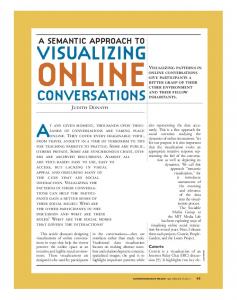
Figure 1. An Example of a Problem Graph
The problem graph is an undirected graph, GProblem = (VP, EP). The set of nodes, VP, of the graph contains a set of problems (i.e., P) reported in the repository. We consider problem reports to be the same if they have the same call stack recorded when the problems are triggered. The set of edges, EP, contains undirected edges, eab={Pa, Pb} if problem Pa and problem Pb are reported together by one or more user. Each user reports both problems (i.e., Pa and Pb). If a large number of users report the two problems together, then we believe that such a relation needs to be highlighted to developers for further investigation. The graph is designed so that only nodes with a direct edge have a relationship. For example, the interconnected nodes P1, P5 and P6 indicate that all three problems have been reported although not necessarily all together. Moreover, there could have been three different users reporting each pair of problems (i.e., {P1, P5}, {P5, P6} and {P1, P6}) or one user reporting the three problems together (i.e., {P1, P5 , P6}}. A problem node appears in the problem graph only if it is reported together with at least one other problem node by a user. We add weights to the nodes and edges. The weight of a node indicates the frequency of unique occurrences of that problem among users in the field testing repository. Visually, nodes are shown as circles with the weight of a node depicted as the size of the circle. Looking at Figure 1, P1 is reported by more users than P3. We define the weight of edges using statistical filtering techniques. We discuss it in Section II.D. Table I summarizes the definition of nodes and edges for the Problem Graph. B. User Graph: Visualizing the Interaction among Users Given the complexity of modern enterprise applications, the usage patterns between users tend to vary considerably with users forming clusters based on their usage of the
application. For example, given an application for order taking and fulfillment, we would expect that at least two user clusters would arise along the two main uses of the application (i.e., order taking and fulfillment) with many sub-clusters forming based on the peculiarities of use within the two large clusters. Different clusters might also arise from commonalities across the user population. Similar characteristics such as similar hardware configuration or usage patterns (e.g., living in areas with bad wireless coverage or slow internet connections) are likely to lead users to report similar problems. Flagging users with common problem profiles is of great value to developers. Using this knowledge about user clusters, developers could replicate specific problems and verify their fixes in an easier fashion. For instance, if most users in the order-taking department have the same problem profile, then a developer might be able to recruit a particular user to deploy additional monitoring on their installation. Developers can work closely with that user to solve a problem that affects the whole cluster of users in the ordertaking department. Furthermore, using this knowledge about user clusters, managers can optimize their planning of future field testing efforts by picking at least one representative user from each cluster to participate in the field testing for a particular software version. Given the limited number of users that are willing to participate in field testing efforts and the large number of releases that are usually tested in parallel, a field-testing manager can distribute their user base more strategically. For example, if there are three versions of the software under testing and prior field testing shows the existence of two distinct user clusters, then the manager should ensure the participation of one user from each cluster to the three tests instead of randomly picking users.
example a user that reports the same problem with four other users has a greater weight than a user who reports two common problems with one other user. Visually, nodes are shown as squares with the weight of a node depicted as the size of the square. Looking at Figure 2, User1 reports more problems in common with other users than User3. We define the weight of edges using statistical filtering techniques. We discuss it in Section II.D. Table I summarizes the definition of nodes and edges for the User Graph. C. Interaction Graph: Visualizing the Relations between Problems and Users The interaction graph gives a global view of the results of field testing process. The graph cross references the relationship between problems and users. The interaction graph helps analyze the visualization produced by the other two graph types. For example, while the problems are not identified within the user graph, the interaction graph could be used to cross-reference the specific problems after locating a particular user base in the graph. The interaction graph is an undirected, weighted graph, GInter =(VI, EI). The set of nodes, VI, is the union of the user set (i.e., U) and the problem set (i.e., P). Figure 3 illustrates an example of the interaction graph. The circular nodes represent problems and the square nodes represent users. The set of edges, EI, contains an undirected edge, eab={Pa, Userb}, if Userb reports a problem, Pa. For the example shown in Figure 3, User3 and User7 both report problems P2 and P3. P1 is reported by User1, User2 and User3.
Figure 3. An Example of an Interaction Graph
Figure 2. An Example of a User Graph
We developed the user graph to help identify such clusters. The user graph is an undirected graph, i.e., GUser = (VU, EU). The set of nodes, VU, of the user graph contains a set of users (i.e., U) who report problems sent to the repository. The set of edges, EU, contains an undirected edge eab={ua, ub} if users, ua and ub, have reported at least one common problem. The weight of a user node represents the number of unique problems that a user reports with other users. For
The weight of a user node captures the number of unique problems reported by the user. Visually, the weight of a user node is shown as the size of the square node. The weight of a problem node reflects the frequency of the problem occurred during the field testing. Visually, the problems are depicted as circles with the weight of a node illustrated as the size of the circle. As depicted in Figure 3, User8 reports more problems than User1. Problem P2 occurs more frequently than problem P1. We define the weight of edges using statistical filtering techniques. We discuss it in Section II.D. Table I summarizes the definition of nodes and edges for the Interaction Graph. D. Statistical Filtering and Weighting Showing all the users and problems that exist in a field testing repository would lead to very complex graph with
TABLE I.
Graph Problem Graph
User Graph
Entity Node
Entity type Problem
Edge
Both problems co-occur
Node
User
Edge
Both users report the same problems
Node
Problem, User
Edge
User reports the Problem
Interaction Graph
SUMMARY OF THE THREE TYPES OF GRAPHS
Weight The number of different users who report the problem at least once in the repository Statistical weight (see section II.D)
Filtering Must co-occur with at least one other problem after edge filtering Statistical filtering (see section II.D)
The number of unique problems that a user has in common with other users Statistical weight (see section II.D)
Must report a single problem after edge filtering. Statistical filtering (see section II.D)
Problem: The number of times a problem is reported by any user User: The number of unique problems reported by a user Statistical weight (see section II.D)
Same as above for problem and user nodes
high over plotting. Therefore we chose to filter the edges and nodes in the created graph. Traditionally such filtering is performed by showing edges which are above a particular threshold. For example, we could show edges between nodes which exhibit a co-occurrence relation 70% of the time or based on basic counts (e.g. 70 times). Instead we choose to perform statistical filtering given the large size of the data. The goal of our statistical filtering is to only show edges that do not simply occur due to chance, instead we want to show edges that indicate statistically significant relations (i.e., association). We perform a chi-square (χ2) test on each edge and filter edges in all graphs based on the results of the test [9]. Table II shows the 2x2 contingency table used to calculate the chi-square value. The same approach is used for all three graphs. For example, in the problem graph, the cell (Pa, Pb) counts the frequency (i.e., f1) where problems Pa and Pb appear together for any users. The cell (Pa, ¬Pb) counts the number of times (i.e., f2) that problem Pa occurred but not problem Pb for a user. The cell (¬Pa, Pb) counts the number of times (i.e., f3) that problem Pb occurs but not problem Pa. The cell (¬Pa, ¬Pb) denotes the total number of times (i.e., f4) that neither problem is reported. χ2 is calculated using formula (1). Looking at the chi-square (χ2) statistics distribution tables, we use a chisquare value of 5.99 to filter edges, indicating that we are 95% confident (i.e., p value