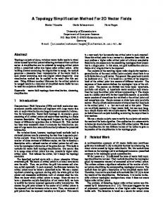
Wrapping of monkey saddle onto trisector point that the local flow structure in the vicinity of nonlinear vector field singular- ities always consists of a set of ...
Visualizing the Topology of Symmetric, Second-Order, Time-Varying Two-Dimensional Tensor Fields Xavier Tricoche1 , Xiaoqiang Zheng2 , and Alex Pang2 1 2
University of Utah, Salt Lake City, UT 84112, USA University of California, Santa Cruz, CA 95064, USA
Abstract. We introduce the underlying theory behind degenerate points in 2D tensor fields to study the local flow characteristics in the vicinity of linear and nonlinear singularities. The structural stability of these features and their corresponding separatrices are also analyzed. From here, we highlight the main techniques for visualizing and simplifying the topology of both static and time-varying 2D tensor fields.
1 1.1
Fundamental notions of two-dimensional tensor field topology Basic definitions
Eigenvector fields. We consider symmetric, second-order two-dimensional, real tensor fields that we term tensor fields hereafter. The tensor values of such fields correspond to symmetric, linear transformations that map vectors to vectors in the plane. When considered in a Cartesian coordinate system, tensor fields can be represented by matrix-valued functions mapping points to 2 × 2 symmetric matrices. Tensor fields are fully characterized by their real eigenvalues and orthogonal eigenvectors. Hence the basic idea behind tensor field topology is to analyze the qualitative properties of a tensor field through the structure of its associated fields of eigenvectors. To formalize the notion of tensor topology, one needs a systematic way to associate a tensor field with the classified pair of corresponding eigenvector fields. This is done by sorting the eigenvectors according to the real eigenvalues. Definition 1. Let λ1 ≥ λ2 be the two real eigenvalues of the tensor field T, i.e. λ1 and λ2 are both scalar fields as functions of the coordinate vector x. The corresponding eigenvector fields e1 and e2 are called major and minor eigenvector field, respectively. Positions at which λ1 = λ2 are associated with isotropic tensor values and constitute singularities. Line fields and covering spaces Similar to streamlines integrated over vector fields tensor field lines [5] are defined as follows.
2
Tricoche, Zheng, Pang
Definition 2. A tensor field line computed in a smooth continuous eigenvector field, is a curve that is everywhere tangent to the direction of the field. By analogy with vector fields, we associate the set of all tensor field lines in a particular eigenvector field with a mathematical flow. Because of the very nature of eigenvectors, the tangency is expressed at each position in the domain in terms of lines. For this reason, an eigenvector field is essentially a line field. This implies that classical theorems ensuring existence and uniqueness of streamlines cannot be directly applied here. However there exists a fundamental relationship between vector and eigenvector fields that can be formally characterized in terms of covering space. A rigorous introduction to this notion of algebraic topology is beyond the scope of this presentation and we restrict ourselves to an illustration of the basic idea. More details can be found e.g. in [6]. Consider the configuration illustrated in Fig. 1(a). An eigenvector field is defined over the bottom layer. This layer is covered by two similar layers over which two normalized vector fields are defined that point in opposite directions. A projection operator associates every pair of opposite vectors with a single eigenvector (line) direction in the bottom layer. Using this construct, an eigenvector field can be interpreted as the projection of two opposite vector fields. Moreover the path lifting property ensures that streamlines integrated over the vector fields defined in the covering space project onto tensor field lines in the eigenvector field. This eventually provides the theoretical framework for tensor field line integration. We mentioned previously that eigenvector fields become degenerate at
y1
y2
Π
x
(a) 2-fold covering
(b) Branched covering
Fig. 1. Covering spaces
positions where the tensor field is isotropic, that is has two equal eigenvalues. This degeneracy corresponds to a so-called branch of the covering space. In the case of a 2-fold covering of a two-dimensional space, this configuration is equivalent to the complex map z 7→ z 2 defined over the unit ball around zero, as shown in Fig. 1(b). In other words, a degenerate point is associated with a single critical point at the branch point in the covering space through the projection operator.
Visualizing the Topology of 2D Tensor Fields
3
Tensor index. The relationship between vector and tensor fields can also be used to extend the notion of Poincar´e index to the tensor setting. Analogous to the vector case, one defines the index of a closed curve as the number of rotations of the eigenvector fields along this curve. Since these fields are orthogonal the tensor index has the same value for both of them. By continuity of the eigenvector fields, the index of any closed curve will take values multiple of 12 . As a matter of fact, the eigenvector direction reached after full rotation along the curve must be the same as the one we started from. Because of the orientation indeterminacy of eigenvectors, this direction might in fact correspond to a rotation by π of the starting eigenvector. An example is shown in Fig. 2. The tensor index is independent of the coordinate frame. 1 dθ 2π
1 2
e2
λ2
e1
λ1 θ
Fig. 2. Tensor index of a trisector
Moreover it remains invariant under local continuous transformations of the eigenvector field since it takes discrete values. Additionally a curve enclosing a region exhibiting uniform flow has index 0 and the index of a curve enclosing a set of curves is the sum of their individual indices. 1.2
Degenerate Points
According to what precedes, the map associating a tensor value with the corresponding pair of eigenvectors is singular at locations where the tensor value is isotropic. Definition 3. A degenerate point of a two-dimensional tensor field is a location where the field is isotropic. At this position, every non-zero vector is an eigenvector. Because of the indeterminacy of the eigenvectors at degenerate points, tensor lines can intersect there. In the following we successively consider the linear and nonlinear cases. Degenerate points in planar linear fields. A tensor field is called linear if its scalar components are linear functions of the space variable x = (x, y) T . In this case, the linear system providing the position of a degenerate point
4
Tricoche, Zheng, Pang
has a unique solution in general. For the sake of simplicity we assume that the degenerate point is located at the origin of the coordinate system and rewrite the tensor field as follows. µ ¶ α(x, y) β(x, y) T(x, y) = + γ(x, y)I2 , (1) β(x, y) −α(x, y) where γ is the mean value of the real eigenvalues, α(x, y) = α1 x + α2 y and β(x, y) = β1 x + β2 y are linear functions of (x, y), and I2 is the identity matrix. By definition the right term is isotropic and has no influence on the eigenvectors of T. The remaining matrix is called deviator part of the symmetric tensor, denoted D. Observe that it is zero by construction at a degenerate point. To characterize the flow pattern around a linear degenerate point, we extract directions of radial convergence, i.e. tensor lines reaching the degenerate point along straight lines. For convenience we reformulate the eigensystem in polar coordinates, using the fact that it is independent of the distance to the origin in the linear case. We obtain ¶µ µµ ¶¶ µ ¶ cos θ αθ βθ cos θ Dθ eθ × eθ = × = 0, (2) βθ −αθ sin θ sin θ where αθ = α(cos θ, sin θ) = α1 cos θ + α2 sin θ and βθ = β(cos θ, sin θ) = β1 cos θ + β2 sin θ, by linearity. Straightforward calculus yields tan 2θ =
β1 cos θ + β2 sin θ . α1 cos θ + α2 sin θ
(3)
Setting u = tan θ finally leads to following cubic polynomial equation: β2 u3 + (β1 + 2α2 )u2 + (2α1 − β2 )u − β1 = 0.
(4)
Eq. (4) has either 1 or 3 real roots that correspond to angles along which the tensor lines radially reach the origin. These angles are defined modulo π and one obtains 6 possible angle solutions for radial eigenvectors. For a given minor or major eigenvector field, one finally gets up to 3 radial eigenvectors. Consequently the linear case exhibits two major types of degenerate points as shown in Fig. 3. In the case of a trisector the 3 directions computed previously bound so-called hyperbolic sectors, as defined in the next section. In the case of a wedge point, 3 radial directions correspond to the pattern shown in the middle of Fig. 3, while a single radial direction leads to the type depicted on the right. The analysis of the general, nonlinear case will clarify the special role of radial directions as separatrices of the linear topology. Considering the tensor index, it can be seen that trisectors have index − 21 while both types of wedge points have index 21 . Again, refer to Fig. 2.
Visualizing the Topology of 2D Tensor Fields
5
Fig. 3. Linear degenerate points
Nonlinear degenerate points. The configurations seen previously are in fact the simplest types of degenerate points. Using the notations of Eq. (1) it can be shown that a degenerate point is linear if and only if following condition holds: ¯ ¯ ¯ ∂α ∂α ¯ ¯ ∂x ∂y ¯ (5) δ := ¯ ∂β ∂β ¯ 6= 0. ¯ ∂x ∂y ¯
Observe that determinant δ can also be used to distinguish wedge points from trisectors [3]. To study the geometric properties of tensor lines in the vicinity of a nonlinear degenerate point we return to previous considerations about branched covering spaces, see section 1. It follows from the local structure of the covering space that the vector field defined over it is wrapped by the projection operator around the degenerate point. Refer to Fig. 1(b). For example, Fig. 4 shows the vector field corresponding to a trisector point. Standard results from the qualitative theory of dynamical systems [1] tell us Π
Fig. 4. Wrapping of monkey saddle onto trisector point
that the local flow structure in the vicinity of nonlinear vector field singularities always consists of a set of curvilinear sectors that exhibit one of three possible patterns: • parabolic: streamlines reach the singularity in one direction but leave the neighborhood in the other. • hyperbolic: streamlines leave the neighborhood in both directions. • elliptic: streamlines reach the singularity in both directions.
6
Tricoche, Zheng, Pang
From the preceding discussions, we conclude that the same sector decomposition characterizes nonlinear degenerate points. These sectors are shown in Fig. 5. This relationship leads to following definition of separatrices and topological graph of a tensor field.
Fig. 5. Parabolic, hyperbolic, and elliptic sector types
Definition 4. The boundary curve of a hyperbolic sector in the vicinity of a degenerate point is called separatrix. The set of all degenerate points and associated separatrices is called topology of the tensor field. Back in the linear case, the definition above implies that the radial directions computed previously correspond to the separatrices of linear degenerate points. Observe that in the case of a wedge point with two separatrices, two radial directions are actual separatrices whereas the third one is simply included in the parabolic sector and has no topological significance. Eigenvalues near degenerate points. Although extracting 2D singularities is simple (see section 2), finding 3D degenerate tensors is non trivial, as explained in Chapter 14 by Zheng et al. A 3D degenerate tensor is similarly defined as one with at least two equal eigenvalues. Since 3D degenerate tensors are defined solely on eigenvalues, one might be tempted to calculate the eigenvalues at each point and try to find those that are equal. Although the issue is raised in 3D, we explain the difficulty in a 2D context. Previous approach is not viable because the eigenvalues are sorted on each grid point. Unless the singularity coincides with the data point, the majors are always larger than the minors at the data points. There is no way to find the points where the major equals the minor just from the interpolated eigenvalues. Of course one may blame the sorting step. For example, in Figure 6(A), we plot the eigenvalues on a line passing through a degenerate tensor. The solid line represents the major eigenvalues and the dotted line the minor. If we know the major and minor at discrete points, we cannot recover the degenerate points; but if we switch the order of the major and the minor after the degenerate tensor as in Figure 6(B), and have the two groups of eigenvalues on discrete points, we can recover the singularities through interpolation on each group. The question becomes: can we consistently group the eigenvalues into two groups on a 2D domain, where each of them is differentiable? If this could be done, we could use bilinear or bicubic interpolation on each group to get the eigenvalue fields easily, and then recover the singularities.
Visualizing the Topology of 2D Tensor Fields
7
Fig. 6. Eigenvalues around a degenerate tensor
However, from Figure 6(C), we see that this is impossible. The figure plots the eigenvalues around a degenerate tensor on a 2D domain. Separating the eigenvalues into two differentiable groups, corresponds to separating the structure into two differentiable surfaces. But from Figure 6(C), we see that the eigenvalues around a degenerate point form two conical structures. It is easy to see that there is no way to separate this structure into two differentiable surfaces. This conclusion in 2D is easily extended to 3D. 1.3
Structural stability and bifurcations
In cases where the tensor field depends on an additional parameter (e.g. time), the stability of the topological features described previously becomes an essential notion. In fact, the structures considered previously only correspond to instantaneous states of an evolving topology. Both the position and nature of degenerate points may change as the parameter is modified. They can be created or annihilated, which affects the connectivity of the topological graph. In particular, an important question is the persistence of degenerate points under small perturbations of the underlying parameter. This property is called local stability. Structural transformations are called bifurcations by analogy with the terminology used for vector fields. In the following, we restrict our considerations to simple cases of local and global bifurcations. Structural stability. The observations proposed next follow the line of reasoning used in the qualitative study of vector fields [7]. In the following we provide criteria that determine the stability of degenerate points and separatrices. Degenerate Points. Similar to critical points in vector fields, degenerate points obtained in the linear, non-singular case (i.e. trisectors and wedges) are the only stable ones. As a matter of fact, it can be easily shown that arbitrary small perturbations can transform nonlinear degenerate points into a set of linear degenerate points. The stability of trisectors and wedges is explained by the invariance of the tensor index. The stability of each type of wedge points is due to the fact that they correspond to different sets of solutions of the cubic polynomial in Eq. (4), which are both stables.
8
Tricoche, Zheng, Pang
Separatrices. Proceeding our analogy with the vector case, we may see that separatrices corresponding to the boundary curves of hyperbolic sectors at both ends are unstable. Examples are shown in Fig. 7. The intuitive justifica-
Fig. 7. Unstable separatrices
tion of this assertion is geometric in nature: adding an arbitrary small angular perturbation to the line field around any point along such a separatrix suffices to break the connection. Local bifurcations. Previous considerations now allow us to describe typical bifurcations associated with the instability of degenerate points. Note that we do not consider homogeneous merging, as described by Delmarcelle in [3] since it creates unstable structures. Pairwise Creation and Annihilation. A wedge and a trisector have opposite indices. Therefore a closed curve enclosing a trisector and a wedge has index 0 which suggests that the combination of both degenerate points is structurally equivalent to a uniform flow. The local transition from a uniform flow to a wedge and a trisector is a pairwise creation. The reverse bifurcation is called pairwise annihilation. An example is shown in Fig. 8.
Fig. 8. Pairwise annihilation
Wedge Bifurcation. This type of bifurcation was suggested by the remarks on the structural stability of wedge points. Each type of wedge corresponds to a specific number of real roots of the cubic polynomial in Eq. (4), either 1 or 3. The transition from one type to another implies the appearance or disappearance of a parabolic sector.
Visualizing the Topology of 2D Tensor Fields
9
Global bifurcations. In contrast to local bifurcations, global bifurcations induce changes in the connectivity of the topological graph and typically involve large regions in the domain of definition. The bifurcations mentioned here are related to previous considerations about unstable separatrices. They occur when two separatrices emanating from two degenerate points become closer, merge and then split. At the instant of merging, an unstable connection exists. As it breaks, it forces the swap of both separatrices. This modifies the behavior of most curves in the concerned region. An example is proposed in Fig. 9, involving 2 trisectors.
Fig. 9. Global bifurcation with trisector-trisector connection
2
Basic Topology Visualization
The topological approach was first introduced for the visualization of planar vector fields. Helman and Hesselink pioneered this field in 1989 [8]. They proposed a scheme for the extraction, characterization and depiction of linear critical points. This early work inspired Delmarcelle who extended the original scheme to symmetric, second-order planar tensor fields [4] as part of his work on general techniques for tensor field visualization [3]. The method can be applied to either the minor or major eigenvector field. Basically, degenerate points are searched in the data set on a cell-wise basis, where the interpolation scheme is typically linear or bilinear. The corresponding equations to solve are then either linear or quadratic. To distinguish between wedge points and trisectors, Delmarcelle used the determinant δ. Refer to Eq. (5). He showed that a negative value of δ characterizes a trisector, while a positive one corresponds to a wedge point. The cubic polynomial Eq. (4) yields the angle coordinates of the separatrices. Since angular solutions are defined modulo π, for each of them a test must be carried out to determine which one of both possible orientations actually corresponds to a radial direction in a particular eigenvector field. In the case of a wedge point, special care must be taken if the polynomial has three real roots. Indeed, one of the solutions must be discarded since it lies within the parabolic sector. This is done by retaining the two angles spanning the largest interval smaller than π, since Delmarcelle showed that parabolic sectors are always smaller than π in the linear case [3]. The edges of the topological graph are finally obtained
10
Tricoche, Zheng, Pang
by numerical integration of the separatrices, as tensor lines of the considered line field. Classical schemes for the integration of differential equations like Runge-Kutta [9] can be adapted to ensure consistency of two consecutive directions along the curve. In that way, the problem induced by the direction indeterminacy of eigenvectors can be avoided. Observe however that a small step size is required in the vicinity of degenerate points because of fast changing flow directions. This can be done by assigning the Frobenius norm of the deviator as an artificial norm to the tensor field since it provides a measure for the anisotropy. Delmarcelle also suggested a way to embed the missing information conveyed by the eigenvalues by means of a color-coding scheme applied over a LIC-like texture [2] representing the eigenvector flow as shown in Fig. 11. A possible extension of the original topology extraction technique consists in detecting half-singularities located on the boundary of the considered domain. The purpose of topology analysis is namely to characterize the flow behavior in terms of limit sets of the tensor lines, which leads to a partition of the domain in regions where all contained tensor lines connect the same limit set(s). We saw previously that degenerate points are such limit sets. Yet, dealing with bounded domains implies that the boundary itself must be part of this classification. This line of reasoning has been already considered by Scheuermann et al. for vector fields [10]. The same idea applies to the tensor setting: points where the flow is tangential to the boundary correspond to additional limit sets of the topology. They are associated with new separatrices if the tensor line touching the boundary is bent inward. Simple computation leads to following equation for determining the exact position of a touching point: αβ sin 2θ − β 2 cos 2θ = 0, where α, β and θ are functions of the edge parameterization, and (cos θ, sin θ)T is the normalized direction of the considered boundary edge. The notations correspond to Eq. (1). Usually the restriction of the tensor field along the boundary is linear over each edge. In that case, α and β are linear, too. Solving this quadratic equation while checking if the positions obtained actually lie on the edge (i.e. 0 ≤ t ≤ 1) yields positions of tangential contact.
3
Topology Simplification
Topology-based visualization of symmetric tensor fields usually provides synthetic graph depictions of large and complex data sets while conveying the essential structural information of the considered phenomenon. Unfortunately, in certain cases the intricacy of the flow results in a cluttered representation that exhibits a large number of degenerate points and separatrices. This problem typically arises in the analysis of turbulent data sets where numerous structures of various scales are present. In that case it becomes tedious to distinguish between important properties of the data and insignificant details. Observe that this problem is worsened in practice by typical low-order interpolation schemes (like linear or bilinear interpolation) that cause artifacts.
Visualizing the Topology of 2D Tensor Fields
11
Moreover, noise is frequently present in numerical simulations which introduces additional confusing features. An example is given in Fig. 13. To solve this problem simplification methods are required that discard insignificant features according to criteria specific to the considered application. The corresponding transformation of the topology must ensure consistency with the original to permit reliable analysis of the final results. Two different methods have been designed to tackle this problem, based on two different assumptions about the cause of the topological complexity. 3.1
Topology Scaling
The first approach is of geometric nature. Assuming that the topological complexity is inherent to the data (e.g. we have a turbulent flow) the task consists in clarifying the depiction by highlighting large scale structures while neglecting small scale details. Practically the method is based on the observation that close degenerate points, when seen from the large, cannot be distinguished from another and seem to be merged into a more complex, locally equivalent singularity. From the theoretical point of view, the merging of an arbitrary number of linear degenerate points creates a nonlinear singularity, as discussed in section 1.2. These facts are the basic ingredients of the scheme proposed by Tricoche et al. [12] to scale the topology. The first step of the method provides a segmentation of the domain into regions in which all degenerate points are sufficiently close to another, according to a prescribed proximity threshold. A bottom-up clustering scheme is therefore applied on the positions of the original singularities. The second step replaces in each region the contained singularities by a single one, mimicking their merging. To this end, the grid structure is locally deformed and a degenerate tensor value is assigned to a grid vertex. The interpolation scheme in the new cells ensures that this degenerate point is the only one present in the region. Further, by preserving the original field values on the region boundary, global consistency is maintained. The final step consists in extracting the structure of these nonlinear singularities. This is done by looking for radial flow directions on a cell-wise basis and characterizing the types of the various sectors surrounding the degenerate point (refer to Fig. 5). The separatrices are extracted as bounding curves of hyperbolic sectors and integrated over the whole domain to obtain the simplified topological graph. Results are shown in Fig. 13. 3.2
Continuous Topology Simplification
As opposed to the previous method, the second technique proposed by Tricoche et al. [13] is specifically designed to remove insignificant degenerate points from the topological graph. In other words, the topological complexity is treated as an artifact and must therefore be removed while keeping important properties unchanged. We saw previously how bifurcations locally
12
Tricoche, Zheng, Pang
modify the topology while preserving consistency with the surrounding eigenvector flow. More specifically, a pairwise annihilation consists of the simultaneous cancellation of a trisector and a wedge point. Therefore, imposing such bifurcations on the original data permits to prune undesired features. Practically, the method assumes that the tensor field is defined over a piecewise linear triangulation. First, the topological graph is computed and degenerate points are assigned to pairs of trisectors and wedges. Next, each pair of singularities is associated with a scalar value that evaluates its importance in the overall topology. Any user-prescribed criterion can be used for this purpose. A natural idea is to penalize very close degenerate points since they cause visual clutter. However, application specific knowledge can be applied to weigh individual degenerate points and, by extension, the pairs they belong to. The pairs are then sorted according to their importance and processed sequentially. For each of them, a connected cell-wise region is determined that contains the pair and no other degenerate point. In terms of tensor index, the boundary of the region has index 0 and the enclosed eigenvector flow is uniform. Finally the tensor values at the internal vertices are slightly modified in a way that guarantees that both degenerate points disappear. This deformation is controlled by angular constraints on the new eigenvector values and is based on specific properties of piecewise linear tensor fields. As a result, a pairwise annihilation has been enforced while the surrounding structure is unchanged. The corresponding results for the same data set are shown in Fig. 14. Looking at an enlargement, we can see that preserved features are not affected by the removals taking place in the same area, see Fig. 15.
4
Topology Tracking
Theoretical results show that bifurcations are the key to understanding and properly visualizing parameter-dependent tensor fields: they transform the topology and explain how stable structures arise. Typical examples in practice are time-dependent datasets. This basic observation motivates the design of techniques that permit us to accurately visualize the continuous evolution of topology. An early method was proposed by Delmarcelle and Hesselink [4]. They extended their original scheme for tensor topology visualization to the timedependent case. The method is restricted to a graphical connection between the successive positions of degenerate points and associated separatrices, leading to a connection if consistency was preserved. However no connection is made if a structural transition has occurred and bifurcations are not visualized. Instead, the comparison between successive time steps is used to infer the nature of the corresponding transitions: either creation or annihilation. Tricoche et al. proposed a different approach in [11]. The central idea of their technique is to handle the three-dimensional space made of the Euclidean
Visualizing the Topology of 2D Tensor Fields
13
space on one hand and the parameter space on the other hand as a continuum. The time-dependent tensor data is assumed to lie on a fixed triangulation. A “space-time” grid is constructed by linking corresponding triangles through prisms over the parameter space as shown in Fig. 10(a). The choice
side face annihilation �
t �
�
�
�
�
wedge swap �
�
�
�
�
�
�
�
�
�
�
�
�
�
�
�
�
�
�
�
�
�
�
�
�
�
�
�
�
�
�
�
�
�
�
�
�
�
�
�
�
�
�
�
�
�
�
�
�
�
�
�
�
�
�
�
�
�
�
�
�
�
�
�
�
�
�
�
�
�
�
�
�
�
�
�
�
�
�
�
�
�
�
�
�
�
�
�
�
�
�
�
�
�
�
�
�
�
�
�
�
�
�
�
�
�
�
�
�
�
�
�
�
�
�
�
�
�
�
�
�
�
�
�
�
�
�
�
�
�
�
�
�
�
�
�
�
�
creation
(x,y)
(a) Space-time grid
(b) Cell-wise tracking
Fig. 10. Data structure for topology tracking
of a suitable interpolation scheme permits an accurate and efficient tracking of degenerate points through the grid along with the detection of local bifurcations. More precisely, linear space interpolation ensures that each triangle contains at most a single degenerate point at any position in time. Therefore pairwise creations and annihilations are constrained to take place on the side faces of the prisms which simplifies their detection. The principle is illustrated in Fig. 10(b). Individual degenerate points are tracked over prisms and potential wedge bifurcations are detected in their interior. The corresponding segments are then reconnected and pairwise creations/annihilations are found. The paths followed by degenerate points yield curves over the 3D grid. Separatrices integrated from them span separating surfaces that are obtained by embedding corresponding curves in a single surface. These surfaces are used further to detect modifications in the global topological connectivity: consistency breaks correspond to global bifurcations. See Fig. 16.
References 1. A. Andronov, E. Leontovich, I. Gordon, and A. Maier. Qualitative Theory of Second-Order Dynamic Systems. Israel Program for Scientific Translations, 1973. 2. B. Cabral and L. Leedom. Imaging vector fields using line integral convolution. Computer Graphics (SIGGRAPH Proceedings), 27(4):263–272, 1993. 3. T. Delmarcelle. The Visualization of Second Order Tensor Fields. PhD Thesis. Stanford University, 1994. 4. T. Delmarcelle and L. Hesselink. The topology of symmetric, second-order tensor fields. In IEEE Visualization, pages 140 –147, 1994.
14
Tricoche, Zheng, Pang
5. R. Dickinson. A unified approach to the design of visualization software for the analysis of field problems. Three-Dimensional Visualization and Display Techniques, 1083:173–180, 1989. 6. B. Gray. Homotopy Theory. An Introduction to Algebraic Topology. Pure and Applied Mathematics. Academic Press, 1975. 7. J. Guckenheimer and P. Holmes. Nonlinear Oscillations, Dynamical Systems and Linear Algebra. Springer, 1983. 8. J. Helman and L. Hesselink. Representation and display of vector field topology in fluid flow flow data sets. IEEE Computer, 22(8):144–152, 1989. 9. W. Press, S. Teukolsky, W. Vetterling, and B. Flannery. Numerical Recipes in C, Second Edition. Cambridge University Press, 1992. 10. G. Scheuermann, B. Hamann, K. Joy, and W. Kollmann. Visualizing local topology. Journal of Electronic Imaging, 9(4):356–367, 2000. 11. X. Tricoche, G. Scheuermann, and H. Hagen. Tensor topology tracking: A visualization method for time-dependent 2D symmetric tensor fields, 2001. 12. X. Tricoche, G. Scheuermann, and H. Hagen. Scaling the topology of symmetric second order tensor fields. pages 171–184, 2003. 13. X. Tricoche, G. Scheuermannn, and H. Hagen. Topology simplification of symmetric, second order 2D tensor fields. pages 275–292, 2003.
Fig. 11. Steady 2D tensor field (from [4])
Fig. 12. Discrete Tracking (from [4])
Visualizing the Topology of 2D Tensor Fields
Fig. 13. Original and scaled topology
Fig. 14. Progressive topology simplification by enforced bifurcations
Fig. 15. Local topology simplification
15
16
Tricoche, Zheng, Pang
Fig. 16. Visualization of the complete topology evolution