Volatility persistence and returns spillovers between
Recommend Documents
volatility spillovers between exchange rate changes and stock market returns on six industrialized countries, not including New. Zealand and Australia.
Sep 22, 2015 - to a set of emerging MENA stock markets (namely, Bahrain, Egypt, ..... This may be explained by the exchange rate regime of the Kuwaiti Dinar.
Jul 27, 2010 - Joseph A. Schumpeter (1912) argues that banks can spur technological innovation ... For example, Joan Robinson (1952) states that financial.
Jan 7, 2009 - investigate the relationship between volatility persistence and predictability of squared returns. Keywords: GARCH Models, returns, time series, ...
Therefore, changes in crude oil prices can directly have an impact on stock prices ... UK, Japan, and USA) to oil price shocks, based on the standard cash-flow ...
Therefore, changes in crude oil prices can directly have an impact on stock prices ... UK, Japan, and USA) to oil price shocks, based on the standard cash-flow ...
Feb 13, 2015 - macroeconomic announcements: evidence from crude oil markets, ... volatility transmission is recorded from the oil market to the stock market.
Jan 8, 2015 - 1,2,3 Chair of Agricultural Market Analysis, Department of Agricultural ..... During the adjustment process, higher volatility or longer .... Security Act. It requires a consumption of 136 Billion Lt. by 2022 a more ambitious target.
Mar 26, 2014 - Therefore, moving markets including oil has come into prominence as a crisis and ...... gasoline and heating oil in different locations. The North ...
22 hours ago - Econometric Institute, Erasmus School of Economics, Erasmus University Rotterdam, ..... decrease conditional volatility (see Black [18]).
Jan 9, 2008 - However, a little attention has been given to food markets. .... autoregressive framework in which forecast-error variance decompositions are invariant to ..... Lamb, frozen carcass Smithfield London, US cents per pound,.
May 15, 2002 - Corresponding author: Banco Central do Brasil, DEPEP, SBS Quadra 3, .... Bradesco and Itaú had no missing observations with a total of 2928.
Texas Intermediate (USA), Brent (North Sea), Dubai/Oman (Middle East), and .... WTI and Brent, the light sweet grade category, have spot, forward and futures ...
crude oil and financial markets, based on crude oil returns and stock index returns. .... returns, namely FTSE100 (London Stock Exchange, FTSE), NYSE composite (New ...... NYMEX oil futures, Contemporary Economics Policy, 22, 250-269.
Jun 16, 2017 - India Implied Volatility Index, Asymmetric Volatility-Return Relation, ..... Stock Exchange (NSE), the Securities and Exchange Board of India ...
Jan 8, 2015 - 1,2,3 Chair of Agricultural Market Analysis, Department of Agricultural ..... commodity futures markets does not have a significant impact on spot ...
Dubreuille, S. and H.M. Mai (2009) âImpact of European and American Business Cycle. News on Euronext Tradingâ International Journal of Business 14, 124- ...
on mining stock returns and stock market volatility, and the comovements .... optimize their portfolios using mining stocks due to the importance of this sector ..... 10. 20. 30. 40. Copper price. 2004. 2006. 2008. 2010. 2012. 2014. 4000 ..... 0.5. 0
We find that trading profit volatility is positively correlated with the level of understanding of the market, .... sells that the individual or group make during the total trading period. the game. ..... nation Sheetâ to answer these questions. 1.
lower partial moment models, while Hogan and Warren (1974) and Jahankhani ... Larry Lang, James Moser, Peter Schmidt, Bill Schwert, JFQA Managing Editor ...
Both energy stock returns and volatility may not only be driven by .... According to the results from a VAR model with weekly data, alternative energy corporations.
May 21, 1999 - rise in Ïoe and in the Sharpe ratio (see the column marked .... hours worked in response to a positive technology shock is also .... and labor resources are allocated away from the investment sector and towards consumption.
and forms the basis of one domain of technical analysis today.2 Much of this work ..... LeBaron, B. (1994), 'Chaos and nonlinear forecastability in economics and ...
Volatility persistence and returns spillovers between
The volatility in the gold market was found to be less than that at the oil market before and ... portfolio and hedging strategies via the computation of spillovers between the .... the spread between the 10-year and 2-year Treasury Constant. Maturity rate ... 0.5, where d is the memory (differencing) parameter or the fractional ...
Volatility persistence and returns spillovers between oil and gold prices: Analysis before and after the global financial crisis OlaOluwa S. Yaya a,n, Mohammed M. Tumala b, Christopher G. Udomboso a a b
Department of Statistics, University of Ibadan, Nigeria Department of Statistics, Central Bank of Nigeria, Abuja, Nigeria
art ic l e i nf o
a b s t r a c t
Article history: Received 17 February 2016 Received in revised form 17 June 2016 Accepted 20 June 2016
This paper investigated volatility persistence and returns spillovers between oil and gold markets using daily historical data from 1986 to 2015 partitioned into periods before the global crisis and after the crisis. The log-returns, absolute and squared log-returns series of these asset prices were used as proxy variables to investigate volatility persistence using the fractional persistence approach. The Constant Conditional Correlation (CCC) modelling framework was applied to investigate the spillover effects between the asset returns. The volatility in the gold market was found to be less than that at the oil market before and after the crisis periods. The returns spillover effect was bidirectional before the crisis period, while it was unidirectional from gold to oil market after the crisis. The fact that there was no returns spillover running from oil to gold after the crisis suggested a measure of optimum allocation weights and hedge ratio. The results obtained are of practical implications for portfolio managers and decision managers in these two ways: gold market should be used as a hedge against oil price inflationary shocks; and the volatility at the oil market can be used to determine the behaviour of gold market. & 2016 Elsevier Ltd. All rights reserved.
1. Introduction Recently, there has been a great increase in the literature on gold market dynamics. This is due to the recent global financial crisis that plunged the United States, the United Kingdom and other world economies into recession which forced investors to diversify their investment into gold. Also, the global demand for gold has increased as a result of the lesson learnt by investors (Apergis and Eleftheriou, 2016). There is equally a dynamic relationship between gold and oil prices, and this was more evident during the 2008–2009 crisis. Besides, modelling co-volatilities at oil and gold markets is important for international investors and portfolio managers since it helps to forecast the volatility evolution of the prices of those assets and implement the optimal portfolio and hedging strategies via the computation of spillovers between the markets.
Gold and oil are the most actively traded commodities in the world. Gold is noted as a store of wealth during periods of economic and political instability (Aggarwal and Lucey, 2007) and as a volatile monetary asset commodity (Batten et al., 2010; Lucey et al., 2013). The main importance of oil comes from the industrial perspective and the daily global consumption is about 90 million barrels1. For production process, it is a vital input of production and its price is driven by demand and supply shocks (Lombardi and Van Robays, 2011). For centuries, gold has been considered a leader in the precious metals market. It is an investment which is commonly referred to as a “safe haven” in high-risk financial markets. The price is less susceptible to exchange rate fluctuations, unlike oil prices, which depend significantly on the appreciation/ depreciation of US dollars (Baur and McDermott, 2010). Stock and oil price shocks have been found to greatly affect most of the world's economies. This has led to individuals and government agencies having to revert to investment in gold, since
n
Corresponding author. E-mail addresses: [email protected] (O.S. Yaya), [email protected] (M.M. Tumala), [email protected] (C.G. Udomboso). http://dx.doi.org/10.1016/j.resourpol.2016.06.008 0301-4207/& 2016 Elsevier Ltd. All rights reserved.
1 See 2012 US Energy Information Administration Daily world oil consumption in millions of barrels.
274
O.S. Yaya et al. / Resources Policy 49 (2016) 273–281
it is a durable commodity that does not lose value. Changes in oil price particularly have economic impact and these often raise serious concerns among policy makers around the world, as a result of its negative effect on net oil importing economies. Therefore, investors have shifted towards keeping gold as another source to invest instead of oil and stocks. One of the most obvious channels through which gold and oil markets could be linked together is through inflationary shocks (Hooker, 2002; Hunt, 2006). From the theory of macroeconomics, higher oil price often places upward pressure on the overall price level, particularly in the area of greater production and transportation costs. Then, inflationary expectations may lead investors to see gold as an alternative to oil, in order to hedge against the expected decline in the value of the investment on oil (Jaffe, 1989). Melvin and Sultan (1990) assert that political unrest and oil price changes are significant determinants of volatility in gold prices. Once there is high oil price at the market, the oil exporting countries generate more revenue. Since gold constitutes higher share of their respective portfolios, the demand for gold is pushed up and the price of gold at the market is pushed up. Ross (1989) claims that asset returns exert volatility which depends on the rate of information flow and this information can be incorporated into the volatility-generating process of another market. Different volatility patterns are expected since the information flow and the processing time vary across market. Fleming et al. (1998) argue that cross-market volatility can be employed to transmit information and cross-market hedging across markets over time. Understanding the complex relationship between oil and gold, and/or with the rest of the economy is more important. This can be viewed in terms of prices (values at their levels) or looking at the variance and co-volatility, that is the anticipated volatility and shock spillovers between the returns of two financial asset prices. The uncertainties in shocks between a pair of these asset prices may be more prevalent, and understanding their possible implications will be of interest to both investors and policy makers (Salisu and Oloko, 2015). Therefore, stakeholders in these financial markets are usually concerned with the relationships among these prices, particularly the returns and shocks spillovers among them. The analysis of the spillover effects among asset prices provides useful information on how the fluctuations among returns, at mean and variance equations levels, will affect the economic activities and portfolios maximisation by the government and investors. Also, with the current bearish behaviour of oil price at the international markets, it is of interest to study the relationship between oil price and gold prices. We were motivated to look at this gap owing to the fact that oil prices affect gold prices both at price and variance series levels (Gil-Alana and Yaya, 2014). This paper considered the persistence of volatility and returns spillover effects between the prices of oil and gold. The analysis was carried out for periods before and after the global financial crises. The fractional persistence approach and univariate volatility modelling were applied in measuring volatility persistence in the returns and conditional volatility series, respectively. The Constant Conditional Correlation (CCC) multivariate GARCH framework was used to study the spillovers/transmission of returns between the asset returns series. The paper is structured as follows: Section 2, which comes immediately after this introduction, reviews the time series methodology applied in the paper, which includes the fractional persistence and multivariate GARCH modelling approaches. Section 4 presents the data, empirical analysis and the results. In Section 4, we infer from the results obtained in Section 5 the management of gold prices in the presence of oil risk; this is investigated using estimates of optimum portfolio weight and hedge ratio. Section 6 renders the concluding remarks and policy implications.
2. Review of relevant literature Historical time series of international gold price has a close relationship with that of oil price, and different statistical tools have been employed to investigate this relationship (Aruga and Managi, 2011; Zhang and Wei, 2010; Chan et al., 2011). Lamoureux and Lastrapes (1990) aver that standard GARCH models tend to overestimate the underlying volatility persistence when a break is not allowed in the long time series. Bampinas and Panagiotidis (2015) examined the causal relationship between crude oil and gold prices during pre-crisis and post global crisis periods and found, for the pre-crisis period, that causality was linear and only runs from oil to gold, while, at the post global crisis period, the causality was nonlinear and bi-directional. Fernandez (2010) applied Geweke and Porter-Hudak's (GPH) semi-parametric method and periodogram regression-based method of fractional integration and found anti-persistence measure of gold returns. Chkili (2015) applied the bivariate Fractionally Integration GARCH (FIGARCH) model to investigate the dynamic relationship between the mean and variance time series of gold and oil prices. The results indicated the significant dynamic time varying correlation between the two markets and gold seemed to be less persistent. There is the need to study the market surge between the two asset prices in terms of volatility using the variants of bivariate Generalised Autoregressive Conditional Heteroscedasticity (GARCH), with its univariate version proposed in Bollerslev (1986). This is the Multivariate GARCH (MGARCH) model with constant or dynamic conditional correlation and covariance matrices, such as the full parameterised BEKK model (Baba et al., 1989), the CCC or Dynamic Conditional correlations (DCC) model. These models are flexible and efficient in studying the time-varying correlations and returns spillover effects between two asset prices, which is not possible in the case of univariate GARCH modelling frameworks2. Choi and Hammoudeh (2010) applied the DCC model to study the time volatility and correlations in the returns of Brent oil, copper, gold and silver and the S&P500 index. They found increasing significant correlations among all the commodities since the 2013 Iraq war but decreasing volatility correlations into S&P500 index. Kiohos and Sariannidis (2010) explored, in the short run, the effects of oil and financial markets on the gold market. They used a GJR-GARCH model in testing the relationships between them using daily data from January 1, 1999 to August 31, 2009. Their findings showed that the oil market had positive influences on the gold market, and indicated volatility persistence in the gold market. Singh et al. (2011) analysed the time-varying volatility in crude oil, heating oil, and natural gas futures market. They incorporated changes in important macroeconomic variables and major political and wealth-related events into the conditional variance equations. Their results showed that, among the macro variables considered, the spread between the 10-year and 2-year Treasury Constant Maturity rate had a positive relationship with the volatility of all commodities. Ciner et al. (2013) investigated return relations among stocks, bonds, gold, oil and exchange rates, taking data from the US and the UK. Their results showed significant relationship between oil and gold, whereas weak relationship was found in the case of gold with both UK and US exchange rates. Owing to this fact, gold was placed as a safe-haven commodity against exchange rate shocks, while it was not placed as a safehaven commodity against oil price shocks. Ewing and Malik (2013) considered daily samples between July 1993 and June 2010 for multivariate GARCH models in order to 2 See Baba et al. (1989), Bollerslev (1990), Engle (2002), Engle and Ng (1993), Engle and Kroner (1995), Kroner and Ng (1998) and Tse and Tsui (2002).
O.S. Yaya et al. / Resources Policy 49 (2016) 273–281
examine the volatility transmission between gold and oil futures, incorporating structural breaks. They found strong evidence of significant volatility transmission between gold and oil price returns in the presence of structural breaks. Mensi et al. (2013) applied VAR-GARCH to investigate the returns and volatility transmission between the S&P500 and commodity price indices for energy, food, gold and beverages for the period 2000- 2011.They found significant volatility transmission between the S&P500 and commodity markets. The results further revealed highest correlation between the S&P500 index and gold prices, and between the S&P500 index and WTI oil price. Shams and Zarshenas (2014) found evidence of co-movements in gold, oil prices and exchange rates based on copular functions and applications of GARCH models.
275
parameters. These were the log-periodogram regression and the local Whittle estimation, also known as the Gaussian semi-parametric estimation methods. Initially, the log-periodogram method was proposed in Geweke and Porter-Hudak (1983), but a refined version of the estimator is given in Robinson (1995a).4 The method defines the spectral ordinates λ1, λ2, ... , λ m from the periodogram of Xt that is IX ( λk ), and k = 1, 2, ... , m, where m, a bandwidth which increases slowly with n. The log-periodogram regression is then given as:
log⎡⎣ IX ( λk )⎤⎦ = a + b log( λk ) + vk
(6)
where vk is assumed to be i.i.d. Then, the differencing parameter is ^ estimated from the least square estimator b as:
1^ ^ d=− b 2 3. Methodology
(7)
This estimator is asymptotically normal and correspond to the −1/2
3.1. Long memory process and fractional persistence technique Granger and Joyeux (1980) and Hosking (1981) define long memory process3 for both time and frequency domain approaches. The time domain uses a stationary time series process Xt with an autocovariance function
γ(k ) = Cov(Xt , Xt + k ) =
E(Xt , Xt + k )
(1)
. The Gaussian semi-paratheoretical standard error π ( 2πm) metric estimation is based on local Whittle estimator of Kunsch (1987), which is further developed in Robinson (1995b). In the frequency domain, the authors defined, −1
I ( λk ) ∼ e f ( λk )
with θ = ( C , d) and at zero frequency, m
at lag k that is independent of t, then long memory exists if,
γ ( k ) ∼ cγk 2d − 1,
as k → ∞
L( C , d ) = (2)
for 0 < d < 0.5, where d is the memory (differencing) parameter or the fractional difference parameter. The constant cγ is positive finite, 0 < cγ < ∞. Therefore, as the number of lags increases to infinity, the dependence between events apart diminishes very slowly in an hyperbolic decay. Short-range dependence is characterised instead by quickly decaying correlations at an exponential rate to zero as in Autoregressive Moving Average (ARMA) and Markov processes. The asymptotic behaviour in definition (2) means that the autocovariances are not summable, that is,
(8)
⎡
∑ ⎢⎢ log C − 2d log( λk) +
k=1 ⎣
I ( λk ) ⎤ ⎥ Cλk−2d ⎥⎦
(9)
By minimisation, we obtain the Gaussian semi-parametric estimator as,:
⎛ ⎞ m ⎡ m ⎧ ⎫ ⎪ I ( λk ) ⎤⎪ ^ ⎬ − 2dm−1 ∑ log( λk )⎟ d = arg min⎜⎜ log⎨ m−1 ∑ ⎢ −2d ⎥⎪ ⎪ ⎟ ⎢ ⎥⎦⎭ ⎩ ⎝ ⎠ k = 1 ⎣ λk k=1
(10)
Robinson (1995b) notes that this estimator is consistent for d ∈ ( −0.5, 0.5). Although the log-periodogram regression approach is widely applied, its consistency at nonstationary range, d ≥ 0.5, is far less than that of the Gaussian semi-parametric approach.5
∞
lim
n →∞
∑ γ ( k) = ∞ k =−∞
3.2. Multivariate volatility modelling
(3)
In the frequency domain, long memory process is then defined as:
f ( λ ) ∼ cf λ −2d ,
as λ → 0
(4)
implying that the spectral density will be unbounded at low frequencies. For example, at λ = 0, there is a blow-up of the spectral density f ( λ) at the origin and this implies having a pole at frequency zero, that is,
f ( 0) =
1 2π
∞
∑ γ ( k) = ∞ k =−∞
(5)
Different estimation methods for estimating and testing the fractional persistence parameter have been proposed in the literature. These are classified as non-parametric, semi-parametric and parametric methods. In this paper, both semi-parametric and parametric methods were employed. Two semi-parametric methods were first applied in estimating the differencing 3 Long memory is often used interchangeably as long-range dependence, strong dependence or persistence. This is a special case of fractional dependence −0.5 < d < 0.5; hence long memory is a subset of this range.
Following Bollerslev (1990), we define a bivariate CCCMGARCH model specification involving two asset returns, A and B, for both conditional mean and variance equations thus:
rt = Φ + Θrt − 1 + εt ,
(
εt = Dt zt
(11)
)
where rt = rtA, rtB ′ with rtA and rtB being the returns on asset price A and B at time t, respectively; Θ is a ( 2 × 2) matrix of coefficients ⎛ θ11 θ12 ⎞ of the form Θ = ⎜ ⎟; Φ is a ( 2 × 1) vector of constant terms ⎝ θ21 θ22 ⎠
(
)
(
and
identically
)
of the form rt = ϕ A , ϕB ′; εt = εtA, εtB ′ with εtA and εtB being the error terms from the mean equations of the two asset markets, A and B, respectively; zt = ztA, ztB ′ is a ( 2 × 1) vector of in-
(
dependently
)
distributed
errors6;
and
4 The version of the GPH estimator by Robinson (1995a) is implemented in statistical packages for computing fractional dependence parameters. 5 Extensions of the log-periodogram and Gaussian semiparametric methods can be found in Velasco (1999a, 2000) for the log-periodogram estimate, and in Velasco (1999b), Velasco and Robinson (2000), Phillips and Shimotsu (2004, 2005), Abadir et al. (2007) and others for the Gaussian semiparametric method. 6 Note, zt can follow normal, Student t or Generalised Error distributions, and we assumed normal distribution in this work.
276
O.S. Yaya et al. / Resources Policy 49 (2016) 273–281
Dt = diag
(
htA ,
htB
) with h
A t
and htB being the conditional var-
iances of rtA and rtB , respectively. The parameters θ12 and θ21 in the matrix Θ then measures the return spillover effects from asset price B to asset price A, and asset price A to asset price B, respectively. The variance equation is specified as:
htA ρA, B
Ht = Dt′zt zt′Dt = Dt′RDt =
htB
( i = A, B )
(13)
where ω > 0, α ≥ 0 and β ≥ 0 are the parameters in the model, conditioned in order to realise stationary and mean reverting conditional volatility of the shocks in the return series. Since the shock reverts itself to a more stable state, we obtain the persistence of volatility for each conditional variance series and half-life thus:
Persistence = α + β
(14)
Half−life = ln( 0.5)/ln( α + β )
(15)
The smaller the persistence, the smaller the market volatility and half-life gives the period of time the persistence of volatility is halved. In modelling CCC-MGARCH specification, apart from the preliminary exploratory data analysis, tests for serial correlation and ARCH effects, the CCC specifications tests are necessary. These are tests for asymmetry and CC tests. The asymmetry test is the sign and size bias test of Engle and Ng (1993) that set the null hypothesis of symmetric model specification against the alternative of asymmetric specification. In a case where asymmetry is present, we consider the Glosten, Jaganathan and Runkle (GJR-GARCH) specification of Glosten et al. (1993):
hti = ωi + α iεt2− 1 + β i hti− 1 + γ iItiεt2− 1
N
L(Θ) =
( i = A, B )
(16)
where Iti = 1 if εti− 1 < 0 and Iti = 0, otherwise. If γ i is positive and statistically significant, it implies that negative shocks increase the volatility of the series more than positive shocks of the same magnitude. The CCC test of Engle and Sheppard (2001) allows one to make a choice between CCC and Dynamic Conditional Correlation (DCC) model of Engle (2002). The DCC model allows for dynamic correlation, that is, Rt (in (2)), hence we re-write,
Ht = Dt Rt Dt
∑ lt(Θ)= − N ln( 2π ) − t=1
1 − 2
(12)
where Dt is as defined earlier in the mean specification with htA and htB defined as any univariate GARCH(1,1) variant,
hti = ωi + α iεt2− 1 + β i hti− 1
3.2.1. Estimation approach Given a sample of N observations, the parameters of thee bivariate CCC and VARMA-MGARCH model are estimated by maximising the log-likelihood function:
1 2
N
∑ ln Ht( θ ) t=1
N
∑ ε′t ( θ )Ht−1εt( θ )
(20)
t=1
where θ is the parameter vector of the model. The log-likelihood function is maximised by Berndt et al. (1974) algorithm and parameter vector, θ estimated via quasi maximum likelihood estimation.
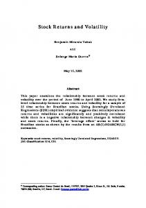
4. Data, empirical analysis and discussion The data considered in this paper were the daily time series of gold and crude oil close prices, given in US dollars per troy ounce and US dollars per barrel, respectively. The gold prices were the set prices at London Bullion Market Association (LBMA), while crude oil prices were the prices at the West Texas Intermediate (WTI) market. Both series were retrieved from Federal Reserve Bank of St. Louis online database at www.stlouisfed.org. The LBMA and WTI markets were considered since these are well known international markets for the pricing of the two asset prices. Data spanning between 2 January 1986 and 8 September, 2015 were obtained. Plots of gold and oil prices are given in Fig. 1. Abreak date corresponding to the onset of global financial crisis on the oil price was observed. This date was around February 2008 based on our data, and this partitioned the graph into panels A and B, corresponding to pre- and post-global financial crisis. Steady fluctuations in the gold prices before the global crisis were observed, whereas these prices fluctuated quite more after the crisis. Differences in the fluctuations in prices of oil before and after the crisis were not observed. These fluctuations are the volatilities in prices experienced over time, and these are better observed in the log-returns series. Investors and stakeholders are interested in market stability than actual prices. Fig. 2 presents the plots of the returns for the two asset prices. By placing the two plots on the same time series scales, as observed on the left for gold returns and on the right side for oil returns, less turbulence was found for gold returns, implying lesser volatility across the time points. When panels C 160
(17)
then,
120
{ ( )} { (
R = Dt−1HtDt−1 = diag
diag
htA ,
htB
htA ,
htB
−1
)}
Ht
2,000
−1
1,600
40
(18)
and, Ht = ( 1 − π1 − π2)H0 + π1εt − 1εt′− 1 + π2Ht − 1, where π1 and π2 are the parameters to deal with the effects of previous shocks and previous dynamic conditional correlations on the current dynamic conditional correlation, and these scalar parameters are non-negative, and H0 is the unconditional variance computed as:
H0 = ω/( 1 − α − β )
80
(19)
By imposing the restriction π1 = π2 = 0, Ht in (20) reduces to a constant, H0 .
1,200 0
A
800
B
400 0
86
88
90
92
94
96
98
00
GOLD
02
04
06
08
OIL
Fig. 1. Plots of daily gold and oil prices.
10
12
14
O.S. Yaya et al. / Resources Policy 49 (2016) 273–281
.2 .0 -.2
D
C
.2
-.4
.0 -.2 -.4 86
88
90
92
94
96
98
00
GOLD
02
04
06
08
10
12
14
OIL
Fig. 2. Plots of Log-returns for gold and oil prices.
and D were considered for the corresponding periods before and after the global crisis, no clear differences were observed in the volatility persistence between each panels. A descriptive analysis was then conducted on the prices (gold and oil), Pt and returns, rt for periods before and after the global crisis, and for full sample, as presented in Table 1. For the period before the global crisis in the upper panel, the average prices for gold and oil were $389.7 and $28.3, respectively, over the entire period. The log-returns were then computed at 1.76E-04 and 2.15E-04, respectively. After the crisis period, the average gold price was computed at $1279.5 and oil price at $87.3, Table 1 Descriptive statistics. Statistics
Before crisis Mean Median Maximum Minimum Std. Dev. Skewness Kurtosis Jarque-Bera
After crisis Mean Median Maximum Minimum Std. Dev. Skewness Kurtosis Jarque-Bera
Full sample Mean Median Maximum Minimum Std. Dev. Skewness Kurtosis Jarque-Bera
indicate the significance of Jarque-Bera statistic at 1% levels.
277
with average returns of 1.11E-04 and 3.29E-04. The average prices for the period after the crisis were higher than that those before the crisis for the two assets. The average returns for gold price were smaller than those of oil in each of the sub-sample considered. This implies smaller volatility persistence than oil price. The average return was smaller for gold after the crisis period. This implies lesser volatility persistence during the period. The average returns for oil were higher after the global crisis; this explains the current oil shocks that are being experienced. With regard to the overall sample, the average price of gold was $617 and that of oil was $42.9. The corresponding average returns were computed at 6.92E-05 and 3.29E-05. The result, was contrary to the previous results for the subsamples. But looking at the estimates of standard deviation of returns, 0.0049 and 0.0109 for gold and oil, respectively, and since that of gold was smaller, we can say that gold prices actually exhibited lesser variations in prices. This is confirmed by the computed maximum and minimum returns for gold and oil prices. For the subsamples and the full sample, normality tests (skewness, kurtosis and Jarque-Bera statistic) indicated that the distribution of the prices and returns were not normally distributed since normality was significant at 5% level. The skewness estimate indicated that prices were rightly skewed while returns series were negatively skewed, except for the oil prices after the global crisis, which was negatively skewed. The results of fractional persistence on the prices, returns, absolute and squared returns, presented in Table 2, starting with periods before global crisis, showed higher persistence in the price of gold than that of oil; whereas the log-returns estimates were negative and closer to zero, indicating un-correlation of returns series. Still in this subsample, in terms of absolute log-returns, gold was expected to experience lesser volatility persistence based on smaller fractional persistence estimates than that of oil. In the period after the crisis, persistence in the prices of gold was found to be marginally higher than those computed for oil, whereas volatility persistence in gold price was lower than that of oil price. This was confirmed by the Gaussian semi-parametric estimate (0.1159) computed for gold, as against 0.0944 and 0.1416 computed for oil based on log-periodogram and Gaussian semi-parametric estimations. As for the full sample, the persistence in the prices of gold was still higher than those computed for oil using the two estimation methods, but volatility persistence estimates based on the absolute returns for the two estimation methods were less in gold than oil price. Conversely, in the squared returns proxy, the estimates of volatility persistence for gold were not significant at 5%, as computed using the two estimation approaches. The results obtained from sign and size bias test for asymmetry of Engle and Ng (1993) and CCC test of Engle and Sheppard (2001) are presented in Table 3. During the period before the crisis, null hypothesis of symmetry was not rejected for the case of gold price but this was rejected in the case of oil price. After the crisis till the end of the sampled data, asymmetry was significant based on joint test and significant in the case of oil price. In the full sample, the null hypothesis of symmetry was not rejected in the case of gold price, whereas asymmetry was significant in the case of oil price. With respect to the results of Engle-Sheppard CCC test, the null hypothesis of constant correlation was not rejected in the subsample before the crisis, implying that constant conditional correlation existed between the conditional volatility series of oil and gold during the sampled period. Conversely, dynamic constant correlation was present in the bivariate model for series after the global crisis. The overall sample showed that CCC model should be applied in capturing the multivariate volatility dynamics between oil and gold prices. Now that model pre-tests have been conducted, we present in Table 4 the results of the CCC and DCC-MGARCH models. In the
278
O.S. Yaya et al. / Resources Policy 49 (2016) 273–281
Table 2 Estimating d in the I (d) setting using both Log-Periodogram GPH and Semi-parametric approaches. Period
, nn, nnn indicate the significance of Jarque-Bera statistic at 1, 5 and 10% levels, respectively. The ARCH LM tests refer to the Engle (1982) test for conditional heteroscedasticity, while the LB and LB2 imply the Ljung-Box tests for autocorrelations involving the standardized residuals in levels and squared standardized residuals, respectively. The null hypothesis for the ARCH LM test is that the series has no ARCH effects (that is, it is not volatile), while the LB test for null hypothesis is that the series is not serially correlated. The figures in parentheses represent the actual probability values.
where θoil and θgold are the autoregressive parameters of order 1 for oil and gold returns, respectively, and θoil, gold measures the returns spillover from gold market to oil market, and also θgold, oil measures the returns spillover from gold market to oil market. If both spillover parameters are significant, there is a bidirectional spillover effect between the asset prices. The other parameters in the CCC model remained as defined in 11–13. From the results, the estimates of constants from the mean equations for oil and gold prices were not significant at 5% level and similarly for the autoregressive parameter for oil returns series, which was not significant in the three sub-samples considered, implying that the current returns of oil price did not explain the immediate past returns of oil price. In the case of gold price, the autoregressive parameter was significant across the three subsamples considered, This implies that the current returns in gold price can be determined by looking at the immediate past history of the returns. As for the returns spillover parameters, for the case of spillovers from oil market to gold market (θ^ ), during the gold, oil
pre-crisis period, the spillover was negative and significant at 5%. From gold to oil market (θ^oil, gold ), the spillover was also negative and significant, implying bidirectional returns spillover effects between oil and gold markets before the global crisis. After the crisis, the return spillover from oil to gold market was no more significant, whereas there was still negative significant returns spillover effect from gold to oil market. Owing to the larger time series sample size before the crisis, the results obtained from the
O.S. Yaya et al. / Resources Policy 49 (2016) 273–281
Note: ***, ** and * denote statistical significance at 1%, 5% and 10% level. Figures in parentheses represent p-values.
full sample also indicated significant bidirectional return spillover effect between the asset prices. The results of the variance equations actually indicated high volatility effects in the returns series across the three sub-samples considered. The results satisfy the conditions for the existence of ^ , α^ and β^ are all GJR-GARCH modelling, that is, the estimates ω positive in the volatility models for oil and gold prices. The asymmetric parameters, γ^oil and γ^gold , were negative and significant during the pre-crisis period. In the post crisis period and in the full sample, these parameters were also significant. With regard to the estimates of the constant correlation (ρ^gold, oil ) for the pre-crisis period and the full sample, as specified by the CCC test, the correlation was found to be positive in both sub-samples, with that of full sample higher in magnitude. This implies positive relationship between the conditional volatility series of the two financial assets. In the case of the post-crisis period which specified DCC model, the estimates of the parameters π^1 and π^2, that is the parameters dealing with the effects of previous shocks and previous dynamic conditional correlations on the current dynamic conditional correlation, were significantly different from zero, with π^1 ¼ 0.0370 in the range [0.02, 0.25] and π^2 ¼0.9230; that is, in the range [0.75, 0.98] (see Bauwens et al. (2012)).
279
Concerning the estimates of persistence (α^ + β^ ) in the pre-crisis period, the persistence estimates were 1.0039 and 1.0257 at oil and gold markets, respectively, implying that volatility persisted indefinitely in these two markets. At the post crisis period, persistence of volatility in the two markets was 0.9575 and 0.9733 o1, implying that volatility reverted to its mean level in these markets. This takes about 16 days in the oil market and 25 days in the gold market for the effects of the market volatility to be halved. The overall sample showed that volatility at the gold market will persist indefinitely, whereas at the oil market, it will take about 86 days for the effect of the effect of the volatility to be halved.
5. Gold asset management in the presence of oil risk Management of gold asset risk is carried out by portfolio design and hedging strategies. We used these strategies to investigate the potential gains from asset diversification between oil and gold markets. This approach was proposed in Kroner and Ng (1998) and further applied in Arouri et al. (2011), who attempted to minimise the risk without reducing expected returns by using the estimates of the conditional variances and covariances. In essence, we analysed a hedge portfolio of oil and gold assets for periods before and after the global crisis. The investor is interested in minimising the risk of his oil–gold portfolio without reducing the expected returns. Kroner and Ng (1998) define a portfolio weight of holding a commodity/gold as,
woil, gold, t =
woil, gold, t
2 2 σgold , t − σoil, gold, t 2 σoil ,t
2 2 − 2σoil , gold, t + σgold, t
(22)
⎧ 0 if woil, gold, t < 0 ⎪ ⎪ = ⎨ woil, gold, t if 0 ≤ woil, gold, t ≤ 1 ⎪ ⎪ 1 if woil, gold, t > 1 ⎩
(23)
woil, gold, t is the weight of oil in a $1 crude oil/gold portfolio at 2 time t, σoil , gold, t is the conditional covariance between the oil price 2 and gold price, σgold , t is the conditional variance for gold price and
2 σoil , t is the conditional variance for oil price. The optimal weight of gold in the oil–gold market portfolio can be evaluated as 1 − woil, gold, t , and this was computed for periods before and after the crisis. Following Kroner and Sultan (1993) regarding riskminimising hedge ratios between oil and gold, the hedge ratio is given as,
βoil, gold, t =
2 σoil , gold, t 2 σgold ,t
(24)
and low ratio of βoil, i, t suggests that oil risk can be hedged by taking a short position in gold markets. The estimates of optimal portfolio weights and hedge ratios were computed from the conditional variances and covariances of the multivariate GARCH model. Table 5 captures the different results for the pre- and post-crisis periods. At the pre-crisis period, the optimal weight of oil in oneUS dollar of oil–gold portfolio was 9.911%; after the crisis, this Table 5 Estimates of optimal portfolio weights and hedge ratio. Before crisis
After crisis
Full sample
woil, gold, t
0.0991
0.1388
0.1114
1 − woil, gold, t
0.9009
0.8612
0.8886
βoil, gold, t
0.1832
0.4055
0.2454
280
O.S. Yaya et al. / Resources Policy 49 (2016) 273–281
became 13.88%; and for the entire time series sample, this was computed as 11.14%. Conversely, the weights of gold were 90.09, 86.12 and 88.86% for the pre-crisis, post-crisis and for full sample, respectively. This means that, for every one-US dollar investment in oil–gold portfolio, during the pre-crisis period, 9.91cents should be invested, after the crisis, 13.88 cents should be invested, and, when the entire full sample is considered, 11.14 cents should be invested. So, for gold asset allocation in oil–gold portfolio, more investments are expected, that is, 90.09 cents, 86.12 cents and 88.86 cents, respectively in the three sub-samples considered. Now, regarding the hedge ratio estimates, it was found that 18.32% of gold was needed on the average to shorten one US dollar long in oil before the crisis, whereas after the crisis, 40.55% of gold was needed to shorten one US dollar long in oil market. The result obtained here is not surprising since volatility of gold was lower than that of oil at the markets before and after the global financial crisis periods; more investment in gold was actually required. Investors should, therefore, hold more gold in their portfolio in order to have the diversification advantage and reduce the risk without lowering the expected return of their portfolio. Hammoudeh et al. (2011) and Arouri et al. (2015) also recommend that, in order to minimise risk, an optimal portfolio of precious metals should be dominated by gold.
6. Conclusion This paper examined possible volatility persistence and returns spillover effects between oil and gold prices using historical daily prices from 1986 to 2015. The time series was partitioned, with 2008 as the period of the onset of the crisis; therefore, there was series for periods before and after the global crisis and the full sample. Log-returns, absolute and squared returns series were obtained, used as proxies to capture volatility in the two asset prices. Fractional persistence approaches based on semi-parametric log-periodogram regression and Gaussian local Whittle estimation approach showed lower estimates of volatility persistence in the case of gold prices before and after the crisis, implying that gold still serves as “safe haven” among other natural resources. Bivariate volatility modelling via the CCC model variants showed that returns spillovers actually existed between oil and gold markets, and that these spillovers were bi-directional before the crisis of 2008; in 2008–2015, this was unidirectional. Analyzing the volatility persistence, returns and volatility spillovers between oil and gold portfolios can provide useful information for portfolio managers, investors and government agencies, who are concerned with movements in oil and commodity markets, particularly the gold market. The results obtained in this paper can be used to build an optimal portfolio and forecast future oil/gold return volatility. That is, gold market should be used as a hedge against oil price inflationary shocks, and the volatility at the oil market can be used to determine the behaviour of gold market.
Acknowledgements We would like to thank Afees Adebare Salisu for rending useful suggestions during the preliminary stage of the paper. The anonymous reviewers are appreciated for their valuable comments and suggestions. References Abadir, K.M., Distaso, W., Giraitis, L., 2007. Nonstationarity-extended local Whittle
estimation. J. Econom. 141, 1353–1384. Aggarwal, R., Lucey, B.M., 2007. Psychological barriers in gold prices? Rev. Financ. Econ. 16, 217–230. Apergis, N., Eleftheriou, S., 2016. Gold returns: do business cycle asymmetries matter? Evidence from an international country sample. Econ. Model. 57, 164–170. Arouri, M., Jouini, J., Nguyen, D., 2011. Volatility spillovers between oil prices and stock sector returns: implications for portfolio management. J. Int. Money Financ. 30, 1387–1405. Arouri, M., Lahiani, A., Nguyen, D., 2015. World gold prices and stock returns in China: insights for hedging and diversification strategies. Econ. Model. 44, 273–282. Aruga, K., Managi, S., 2011. Tests on price linkage between the U.S. and Japanese gold and silver futures markets. Econ. Bull. 31 (2), 1038–1046. Baba, Y., Engle, R.F., Kraft, D., Kroner, K.F., 1989. Multivariate Aimultaneous Generalized ARCH. University of California, San Diego. Bampinas, G., Panagiotidis, T., 2015. On the relationship between oil and gold before and after financial crisis: linear, nonlinear and time-varying causality testing. Stud. Nonlinear Dyn. Econ. 19 (5), 657–668. Batten, J., Ciner, C., Lucey, B.M., 2010. The macroeconomic determinants of volatility in precious metals markets. Resour. Policy 35 (2), 65–71. Baur, D.G., McDermott, T.K., 2010. Is gold a hedge or a safe haven? An analysis of stocks, bonds and gold. Financ. Rev. 45, 217–229. Bauwens, L., Hafner, C., Laurent, S., 2012. Volatility models. In: Bauwens, L., Hafner, C., Laurent, S. (Eds.), Handbook of Volatility Models and Their Applications. John Wiley and Sons, Inc, NJ. Berndt, E., Hall, B., Hall, R., Hausman, J., 1974. Estimation and inference in nonlinear structural models. Ann. Econ. Soc. Meas. 3, 653–665. Bollerslev, T., 1990. Modelling the coherence in short-run nominal exchange rates: a multivariate generalized ARCH approach. Rev. Econ. Stat. 72, 498–505. Bollerslev, T., 1986. Generalized autoregressive conditional heteroscedasticity. J. Econom. 31, 307–327. Chan, K.F., Karuna, S.T., Brooks, R., Gray, S., 2011. Asset market linkages: evidence from financial, commodity and real estate assets. J. Bank. Financ. 35, 1415–1426. Chkili, W., 2015. Gold-oil prices co-movements and portfolio diversification implications. Munich Personal RePEc Archive, MPRA Paper No. 68110. Choi, K., Hammoudeh, S., 2010. Volatility behaviour of oil, industrial commodity and stock markets in a regime-switching environment. Energy Policy 38 (8), 4388–4399. Ciner, C., Gurdgier, C., Lucey, B.M., 2013. Hedges and safe havens: an examination of stocks, bonds, gold, oil and exchange rates. Int. Rev. Financ. Anal. 29, 202–211. Engle, R.F., 1982. Autoregressive conditional heteroscedasticity with estimates of the variance of United Kingdom. Econometrica 50, 987–1008. Engle, R.F., 2002. Dynamic conditional correlation: a simple class of multivariate generalized autoregressive conditional heteroskedasticity models. J. Bus. Econ. Stat. 20, 339–350. Engle, R.F., Kroner, K.F., 1995. Multivariate simultaneous generalized ARCH. Econ. Theory 11, 122–150. Engle, R.F., Ng, V.K., 1993. Measuring and testing the impact of news on volatility. J. Financ. 48, 1749–1778. Engle, R.F., Sheppard, K., 2001. Theoretical and empirical properties of dynamic conditional correlation multivariate GARCH. Mimeo UCSD. Ewing, B.T., Malik, F., 2013. Volatility transmission between gold and oil futures under structural breaks. Int. Rev. Econ. Financ. 25, 113–121. Fernandez, V., 2010. Commodity futures and market efficiency: a fractional integrated approach. Resour. Policy 35, 276–282. Fleming, J., Kirby, C., Ostdiek, B., 1998. Information and volatility linkages in the stock, bond, and money markets. J. Financ. Econ. Vol. 49, 111–137. Granger, C.W.J., Joyeux, R., 1980. An introduction to long memory time series and fractionally differencing. J. Time Ser. Anal. 1, 15–29. Geweke, J., Porter-Hudak, S., 1983. The estimation and application of long memory time series models. J. Time Ser. Anal. 4, 221–238. Gil-Alana, L.A., Yaya, O.S., 2014. The relationship between oil prices and the Nigerian stock market: an analysis based on fractional cointegration. Energy Econ. 46, 328–333. Glosten, L.W., Jaganathan, R., Runkle, D.E., 1993. On the relation between the expected value and the volatility of the nominal excess return on stocks. J. Financ. 48, 1779–1801. Hammoudeh, S., Malik, F., McAleer, M., 2011. Risk management of precious metals. Q. Rev. Econ. Financ. 51, 435–441. Hooker, M.A., 2002. Are oil shocks inflationary? Asymmetric and nonlinear specifications versus changes in regime. J. Money Credit Bank. 34, 540–561. Hosking, J.R.M., 1981. Fractional differencing. Biometrika 68, 165–176. Hunt, B., 2006. Oil price shocks and the U.S. stagflation of the 1970s: some Insights from GEM. Energy J. 27, 61–80. Jaffe, J.F., 1989. Gold and gold stocks as investments for institutional portfolios. Financ. Anal. J. 45, 53–59. Kiohos, A., Sariannidis, N., 2010. Determinants of the asymmetric gold market. Invest. Manag. Financ. Innov. 7 (4), 26–33. Kroner, K.F., Ng, V.K., 1998. Modelling asymmetric movements of asset prices. Rev. Financ. Stud. 11, 844–871. Kroner, K.F., Sultan, J., 1993. Time-varying distributions and dynamic hedging with foreign currency futures. J. Financ. Quant. Anal. 28, 535–551. Kunsch, H.R., 1987. Statistical aspects of self-similar processes. In: Prokhorov, Y., Sazanov, V.V., (Eds.), Proceedings of the First World Congress of the Bernoulli Society. VNU Science Press, Utrecht, pp. 67–74.
O.S. Yaya et al. / Resources Policy 49 (2016) 273–281
Lamoureux, C.G., Lastrapes, W.D., 1990. Persistence in variance, structural change and the GARCH model. J. Bus. Econ. Stat. 8, 225–234. Lombardi, M.J., Van Robays, I., 2011. Do financial investors destabilize the oil price? European Central Bank, Working Paper No.1346. Lucey, B., Larkin, C., O’Connor, F., 2013. London or New York: where and when does the gold price originate? Appl. Econ. Lett. 20, 813–817. Melvin, M., Sultan, J., 1990. South African political unrest, oil prices, and the time varying risk premium in the gold futures market. J. Future Mark. 10, 103–111. Mensi, W., Beljid, M., Boubaker, A., Managi, S., 2013. Correlation and volatility spillovers across commodity and stock market: linking energies, food and gold. Econ. Model. 32, 15–22. Phillips, P.C.B., Shimotsu, K., 2004. Local Whittle estimation in nonstationary and unit root cases. Ann. Stat. 32, 656–692. Phillips, P.C.B., Shimotsu, K., 2005. Exact local Whittle estimation of fractional integration. Ann. Stat. 33 (4), 1890–1933. Robinson, P.M., 1995a. Log-periodogram regression of time series with long range dependence. Ann. Stat. 23, 1048–1072. Robinson, P.M., 1995b. Gaussian semiparametric estimation of long range dependence. Ann. Stat. 23, 1630–1661. Ross, S.A., 1989. Information and volatility: the no-arbitrage martingale approach to timing and resolution irrelevancy. J. Financ. 44, 1–17.
281
Salisu, A.A., Oloko, T.F., 2015. Modelling oil price – US stock nexus: a VARMA–BEKK– AGARCH approach. Energy Econ. 50, 1–12. Shams, S., Zarshenas, M., 2014. Copular approach for modelling oil and gold prices and exchange rate co-movements in Iran. Int. J. Stat. Appl. 4 (3), 172–175. Singh A., Karali B., Ramirez O.A., 2011. High price volatility and spillover effects in energy markets. Selected paper prepared for presentation at the Agriculture & Applied Economics Association's 2011 AAEA & NAREA Joint Annual Meeting, Pittsburgh, Pennsylvania, July 24–26, 2011. Tse, Y.K., Tsui, A.K.C., 2002. A multivariate GARCH model with time-varying correlations. J. Bus. Econ. Stat. 20, 351–362. Velasco, C., 1999a. Nonstationary log periodogram regression. J. Econom. 91, 325–371. Velasco, C., 1999b. Gaussian semiparametric estimation of nonstationary time series. J. Time Ser. Anal. 20, 87–127. Velasco, C., 2000. Non-Gaussian log periodogram regression. Econ. Theory 16, 44–79. Velasco, C., Robinson, P.M., 2000. Whittle pseudo maximum likelihood estimation for nonstationary time series. J. Am. Stat. Assoc. 95, 1229–1243. Zhang, Y.J., Wei, Y.-M., 2010. The crude oil market and the gold market: evidence for cointegration, causality and price discovery. Resour. Policy 35 (3), 168–177.