1
Voltage Prediction Using a Cellular Network Lisa L. Grant, Student Member, IEEE, and Ganesh Kumar Venayagamoorthy, Senior Member, IEEE
Abstract-- Better identification tools are needed for power system voltage profile prediction. The power systems of the future will see an increase in both renewable energy sources and load demand increasing the need for quick estimation of bus voltages and line power flows for system security and contingency analysis. A Cellular Simultaneous Recurrent Neural Network (CSRN) to identify and predict bus voltage dynamics is presented in this paper. The benefit of using a cellular structure over traditional neural network architectures is that the network can represent a direct mapping of any power system allowing for easier scalability to large power systems. A comparison with a standard single SRN is provided to show the advantages of this cellular method. Two types of disturbance are evaluated including perturbations on the power system generators and on the least stable loads. The method is also evaluated for a case involving a transmission line outage. Index Terms--Cellular Simultaneous Recurrent Neural Network (CSRN), Small Population Particle Swarm Optimization (SPPSO), voltage profile prediction
E
I. INTRODUCTION
arly estimation of power system voltage instability is imperative for reduction of large blackouts. An increase in the trend for interconnections between power systems to reduce cost has led to an increase in complexity for the voltage collapse problem. The main cause of this complexity is that system voltages are operated much closer to their stability limits. As the load demand on a system is increased, voltages that are already operating close the stability limits decrease causing major disturbances and blackouts [1]. For effective voltage stability, a power system must maintain a steady and acceptable voltage level at normal operating conditions, after increase in load, during system configuration changes or when the system is being subjected to a disturbance. The recent trend of deregulated and competitive power markets has also brought about a more complicated network topology because of frequent transactions between generation and distribution companies. This has led to an increase in the potential for high voltage instability in power systems. Voltage instability can be alleviated by implementing adaptive solutions to increase stability margins and improve dynamic control. Traditional methods for contingency analysis include numerous load flow calculations requiring long computation time [2]. Faster prediction methods for assessing voltage stability are needed so that preventative action can be taken before blackouts due This work was supported in part by US National Science Foundation EFRI #0836017 and GAAANN #P200A070504. L. L. Grant and G. K. Venayagamoorthy are with the Real-Time Power and Intelligent Systems Laboratory at Missouri University of Science & Technology, Rolla, MO 65401 USA. (e-mail:
[email protected]).
978-1-4244-6551-4/10/$26.00 ©2010 IEEE
to voltage collapse occur. To achieve this goal, a tool needs to be developed to correctly identify power system voltage profiles under different operating conditions. The focus is to alleviate the effects of the rise in renewable energy sources along with increasing loads causing power system voltage profiles to be constantly changing. It is necessary to adjust power system parameter settings quickly and efficiently in response to these changes. The optimal method of achieving this would be to predict system changes faster than real time so that the necessary controls can be implemented before the system changes occur which will help to reduce or even prevent system disturbances or outages. This requires a method for very fast and accurate power system modeling [3]. Neural networks including multi-layer perceptron (MLP) and radial basis function (RBF) have been used for voltage stability tracking, prediction, and monitoring due to their great ability for pattern recognition [4]. Neural networks use internal connection weights to learn the relationships between inputs and outputs consequently discovering the intricate characteristics of the system under study. This paper describes how a Cellular Simultaneous Recurrent Neural Network (CSRN) structure can be used to predict bus voltage profiles. The CSRN architecture allows for accurate system equivalent modeling and fast prediction. The voltage dynamics of a highly interconnected power system can be directly replicated by the connections between the cells of the CSRN where the cellular connections represent the transmission lines connecting the buses of the power system. Ideally a CSRN can be used to predict system profiles N steps ahead of time. In an online application if a CSRN can predict system voltage profiles N steps ahead, then the system operator has that much more time to implement the necessary controls or run analysis on the system. Preliminary simulation results on the 12-bus multi-machine power system show the performance capabilities of this technique for a single-step prediction. The paper is organized as follows: Section II provides details on the test power system and how CSRNs are used for bus voltage prediction, Section III contains simulation results and discussion for the CSRN and the single SRN for comparison, Section IV includes a discussion and example on how this method can provide voltage stability assessment for power systems, and Section VII contains a conclusion and future direction of this work.
2
Bus 1
Vˆ1 ( t + 1)
Infinite Bus G1 ~
Vˆ10 ( t +1) V10 ( t ) Vˆ5 ( t + 1) V5 ( t )
Vˆ4 ( t + 1)
V1 ( t )
Bus 5 Bus 4
Bus 2 Bus 10 G2 ~ VG2 V2
V10
Area 2
Vˆ2 ( t + 1)
V5 V4
V2 ( t )
Area 3
Vˆ6 ( t + 1)
Bus 6 Bus 9 G4 ~ VG4
Area 1 Bus 7 V6
V9
Bus 8
V7
V8
V9 ( t )
Vˆ9 ( t + 1)
V6 ( t )
Bus 3 Bus 11 G3 ~ VG3
V1
V4 ( t )
V3
V7 ( t )
V11 ( t )
V11 Vˆ7 ( t + 1)
Fig. 1. 12-bus test power system.
II. CSRN BASED VOLTAGE PREDICTION A. Test Power System A small power system was used to test the CSRN for the voltage profile prediction concept. The 12-bus benchmark test power system, shown in Fig. 1, includes six 230-kV buses, two 345-kV buses, and four 22 kV buses [5]. The infinite bus is connected to a 22 kV source. The three area system consists of two hydro-generators (G2 and G4) in areas 1 and 2 respectively, and a thermal generator (G3) in area 3. Parallel transmission lines connect buses 3 and 4. Parameters of the generator and exciters are given in [5]. B. Bus Voltage Prediction The input and desired output data for the neural networks are taken from the power system simulation. The steady state bus voltage values are the bus voltages under steady state conditions with no disturbance added after computing the load flow. For this study the CSRN is used to predict the voltage deviation at each system bus (ignoring the infinite bus). The bus voltage deviations (ΔV1, ΔV2 …, ΔV11) are computed from the measured voltages at each bus subtracted from the steady state values. The inputs to the CSRN are the voltage deviations monitored at each bus of the power system. The output of the CSRN is the predicted voltage changes on each bus at one step ahead in time where each time step is 100 ms. The goal is to have the CSRN be able to accurately model all of the bus voltages correctly for any power system state. For instance if a disturbance results in an increase of generation, the CSRN should respond to the changes in voltage in the same way as the 12-bus power system would behave. C. CSRN Structure For this application a standard Simultaneous-Recurrent Neural Network (SRN) is implemented in each cell of the CSRN and the size of each cell is indicated in CSRN diagram
Vˆ8 ( t + 1) V8 ( t )
V3 ( t ) Vˆ3 ( t + 1)
Vˆ11 ( t +1)
Fig. 2. CSRN diagram showing power system equivalent mapping of bus connections.
show in Fig. 2. Research has been done to show the benefits of Cellular SRNs over feedforward MLPs as many voltage stability prediction studies have been carried out using the MLP network [6]-[11]. CSRNs can improve accuracy and speed of training due to the small size of the NN in each individual cell and the ability to train each cell in parallel. For this application 11 cells are used. Each cell of the CSRN represents one of the buses in the 12-bus system where the infinite bus (bus 12) is ignored. The connections between the CSRN cells represent a direct mapping of the transmission lines connecting the buses in the 12-bus system. Each cell predicts the bus voltage indicated by Vˆi ( t + 1) of bus number i that the cell is representing at the next time step t+1. The inputs to each cell are the actual bus voltage at time t or Vi(t) directly measured from the power system, and the timedelayed predicted voltage outputs of the buses that are connected to the cell at time t or Vˆbus ( t ) . For example, Cell 1 would be used to predict the voltage on bus 1 or Vˆ1 ( t + 1) . The inputs to Cell 1 would be the actual measured voltage of bus 1 or V1(t), and the time-delayed predicted bus voltage outputs of buses 2, 6, and 7 ( Vˆ2 ( t ) , Vˆ6 ( t ) , Vˆ7 ( t ) ) since those buses are directly connected to Bus 1. The benefit of using one cell to predict the voltage of a single bus using inputs from its nearest neighboring buses is that for a larger power system the size of each cell’s SRN will remain small even though the overall number of cells in the network will increase directly proportional to the number of buses in the system. Table I contains information on the size of each cell in the CSRN along with the number of weights in each cell. In a typical power system, the average number of connecting buses is around 4; therefore, the average largest cell in any size power system’s equivalent CSRN would utilize a SRN of size 4x3x1. Scaling to larger system involves adding cells to the CSRN in proportion to the number of monitored system buses. This greatly reduces complexity and computation time when scaling up for larger systems. The
3
training and output of the individual cells can be computed very quickly in parallel with minimal input connections between cells since the size of each cell’s SRN remains small and the training of such a small neural network can be completed in a few seconds. TABLE I SIZE OF EACH CELL WITH NUMBER OF WEIGHTS IN THE CSRN No. Cell/Bus No. Inputs No. Hidden No. Outputs No. Weights 4 3 1 24 1 4 3 1 24 2 4 3 1 24 3 4 3 1 24 4 3 3 1 21 5 4 3 1 24 6 3 3 1 21 7 3 3 1 21 8 2 3 1 18 9 2 3 1 18 10 2 3 1 18 11 35 33 11 237 Total
D. CSRN Training For NN weight training, an advanced form of Particle Swarm Optimization (PSO) known as Small Population PSO (SPPO) is used. Details on the SPPSO algorithm can be found in [12]. Kennedy and Eberhart developed PSO in 1995 [13], [14]. In [15], PSO has been show to be a faster training method than backpropagation for neural networks. This swarm intelligence algorithm is based on the behavior of a school of fish or flock of birds. The collective interactions of the individuals in the swarm allow for more optimal solutions to evolve through time. Each member of the swarm, referred to as a particle, randomly searches the environment while updating its position using its own memory and information gathered from the other particles. The particles are given initial random velocities and ‘flown’ through the problem space. The position that resulted in the particle’s best fitness, known as the Pbest value and the best value of all the Pbest values defined as the global best position, Gbest, are stored in memory. The velocities and positions of the particles are updated every iteration until the swarm has converged on the desired solution. The core of the PSO algorithm is the velocity and position update equations given by (1) and (2) respectively. The constants w, c1, and c2 are adjusted to determine to what degree the current velocity, personal best, or global best position will affect the particle’s next position. The time variable t indicates the current time step in the search.
V (t ) = w *V (t − 1) + c1 * rand1 * ( Pbest (t − 1) − P(t − 1) )
(1)
P(t ) = P(t − 1) + V (t )
(2)
+c2 * rand 2 * ( Gbest (t − 1) − P(t − 1) )
In SPPSO, the same methodology is carried out as in standard PSO, with the addition of a regeneration concept which allows the utilization of fewer particles greatly deceasing computation time while maintaining the diversity of the optimization method. For this application, 5 particles were
used where standard PSO usually requires 20 to 30 particles. Each cell is trained individually so 11 different SPPSO algorithms are used to train the weights of the CSRN, one SPPSO for each cell. The CSRN was trained using pseudorandom binary signals (PRBS) fed into the generators excitation control (buses 9-11) and the least stable loads (buses 3, 4, and 6). The PRBS signals excite the natural frequencies of the system. Training in this manner allows the CSRN to identify the dynamics of the power system. The disturbance signals are formed by using delayed random noise at different frequencies which are summed to create the PRBS signal. For this application, frequencies of 2, 1, and 0.5 Hz were used for PRBS on the generators and frequencies of 0.2, 0.5, and 1 Hz for PRBS on the loads. The PRBS signals on the loads have a magnitude of ±10% of the steady state power rating for each load. E. SRN Structure for Comparison To compare with existing prediction methods, a single SRN is also used to predict the bus voltages of the 12-bus power system. In the Elman SRN, the hidden layer is fed into an input context layer storing previous states of the hidden layer at the previous pattern presentation. This study looks at a standard SRN(size 12x13x11; 468 weights) as a comparison to the CSRN architecture. For the standard SRN pictured in Fig. 3, there are 12 inputs denoted by V, which include the 11 bus voltage deviations (V1, V2, …, V11) and a bias of 1. The outputs of the SRN denoted by Vˆi ( t + 1) are the predicted bus voltages at the next 100 ms time-step. The standard SRN network uses one SRN to predict the voltages of all 11 power system buses. Given the current bus voltages as inputs, the SRN will predict the voltage of each of the 11 buses at the next time step. The voltages of the infinite bus (bus 12) are not considered for this application.
Vˆ
V V1 ( t )
V2 ( t )
Vˆ1 ( t + 1) Vˆ ( t + 1) 2
V11 ( t )
Vˆ11 ( t + 1)
Fig. 3. Detailed Elman SRN model for the 12-bus system. (12 x13 x 11)
4
III. RESULTS A. PRBS on the Generators The Cellular SRN and single SRN were trained using data where all three generators PRBS switches were active. The bus voltage signals were sampled at 10 Hz for a period of 20 seconds, which produced 200 samples of data per voltage waveform at a sampling rate of 100 ms. To show the robustness of this technique, testing was performed on the network after fixing the training weights using data where PRBS signals were only activated on generators 2 and 3. The bus voltage waveform results for CSRN can be seen in Figs. 4 and 5 where the solid line indicates the actual bus voltage measured from the 12-bus system and the dashed line indicates the bus voltage predicted by the CSRN. Figs. 6 and 7 contain results for the single SRN. The results in Figs. 4 and 6 include results for three of the load buses, one bus from each area (bus 2 – Area 1; bus 6 – Area 2; bus 5 – Area 3). The results in Fig. 5 and 7 include results from the three generator buses (bus 9, bus 10, bus 11).
Fig. 4. CSRN testing results for load buses with PRBS applied to the generators.
Fig. 6. SRN testing results for load buses with PRBS applied to the generators.
Fig. 7. SRN testing results for generator buses with PRBS applied to the generators.
B. PRBS on the Loads The natural load changing characteristics of the power system are represented and tested using PRBS signals on the load buses. The PRBS signals applied to system loads replicates the demand side response of the power system. The load buses in the 12-bus system experiencing the lowest voltages during steady state analysis were chosen for the addition of PRBS load disturbances which included buses 3, 4, and 6. Figs. 8 and 9 show the CSRN and SRN results for three of the load buses for PRBS on the weakest loads in the system. As with the first test case, the CSRN method outperformed standard single SRN method. The accuracy was tested even more with load PRBS since the disturbance signals were applied to both real and reactive power waveforms resulting in a more complex voltage pattern then with PRBS on the generators. Fig. 5. CSRN testing results for generator buses with PRBS applied to the generators.
5
Fig. 8. CSRN testing results with PRBS applied to the loads.
Fig. 9. SRN testing results with PRBS applied to the loads.
C. Network Topology Changes To test the CSRN prediction capabilities under network topology changes, one of the transmission lines connecting bus 3 to bus 4 was tripped. Tests using PRBS on the generators and PRBS on the loads to simulate the power system’s natural load changing characteristics were performed on the system with the transmission line outage. The single SRN described in Section II-e was unable predict the voltages for the line outage case. Results showing the CSRN voltage prediction capabilities under a network topology changes can be seen in Figs. 10-11.
Fig. 10. CSRN testing results for transmission line outage with PRBS applied to the generators.
Fig. 11. CSRN testing results for transmission line outage with PRBS applied to the loads.
D. Fitness Measure The fitness criterion for both methods was determined by measuring the Mean Square Error (MSE) of the predicted waveform for each bus relative to the actual measured voltage on each bus. Fig. 12 contains the MSE for each bus of the SRN and CSRN methods for testing with PRBS on Generators and Fig. 13 shows the MSE testing results for PRBS on loads. The charts show the superiority of the CSRN method with all buses’ MSEs being below the single SRN MSEs. The only exception is bus 8’s MSE is slightly worse for CSRN than SRN for PRBS on loads, though the overall prediction accuracy of CSRN for load disturbances is much better for the system as a whole than SRN’s prediction capabilities. IV. APPLICATION OF CSRN FOR VOLTAGE PREDICTIONS CSRNs can be used to predict the health of a power system in terms of voltage profile. This can be performed ahead of time before system changes actually occur so that appropriate steps can be taken to prevent any possible future voltage instability. There are numerous practical applications for this type of tool but the scope this paper is to show that CSRN have potential for predicting Voltage Stability Indices (VSI). Voltage stability indices can be used to predict the system critical operating point with respect to the point of dynamic voltage collapse [17]. Using the CSRN method to determine a voltage stability indicator would allow system operators to quickly determine the security of the current or future operating point for any size of power system and take the correct preventative action without fear of disturbing vital power system processes and components. Preliminary VSI results have been obtained using the Dynamic Voltage Index (DVI) in (3). The DVI includes voltage deviations of all buses within the system where Vn is the rated voltage, vi,min is the minimum instantaneous voltage on the ith bus, vi,min,adm is the minimum admissible voltage value, and nbus is the number of buses being evaluated in the system. Fig. 14 contains the DVI plot at each 100 ms sample for the voltage waveforms of the Actual measured, SRN predicted, and CSRN predicted cases.
6
V. CONCLUSION AND FUTURE WORK
Fig. 12. MSE of each bus for PRBS on Generator Testing.
Fig. 13. MSE of each bus for PRBS on Load Testing.
⎧⎪ max ⎡ Vn − vi ,min ⎤ ⎫⎪ DVI = min ⎨1, ⎢ ⎥⎬; V v − i 1,..., nbus = ⎢ ⎥⎦ ⎭⎪ n i ,min, adm ⎣ ⎩⎪
(3)
Preliminary results have shown that a CSRN is capable of accurately predicting the bus voltage profiles of the 12-bus power system much more accurately than standard neural network based methods. Since the CSRN represents a direct mapping of the power system, this method is easily scalable to larger systems without adding computational complexity and increased runtime. The CSRN was able to provide more accurate predictions than a single SRN network for all system buses using half the number of trained neural network weights. For scaling to larger power systems, each cell in the CSRN would remain small even though cells would need to be added; whereas, prediction using a single SRN for all bus voltages would require an exponential increase in the number of trainable weights as the size of the power network increased. A practical use of this technique has been shown by calculating the voltage stability index, specifically the DVI, for the 12-bus system and comparing the DVIs of the CSRN and SRN predictions. The CSRN is able to track the DVI of the system much more closely than the single SRN indicating that the health of the system can be accurately monitored prior to the initiation of system disturbances allowing for the appropriate preventative measures to be taken before disturbances occur. Future studies will include investigating the potential of CSRN for prediction of bus voltages on larger power systems under different conditions to prove scalability of this technique and determine the computational requirements of scaling to larger systems. Also, comparing the CNN method to other existing voltage prediction techniques will be performed to show the practical applicability of this method. Using the CSRN method to determine a voltage stability indicator would allow system operators to quickly determine the security of the current or future operating point of any size of power system and take the correct preventative action without fear of disturbing vital power system processes and components.
where Vn = 1.0, vi ,min, adm = 0.9
VI. REFERENCES [1] [2]
Dynamic Voltage Index (DVI)
0.85
Actual SRN CSRN
0.8
[3] [4]
DVI
0.75
0.7
[5]
0.65
[6] 0.6
[7] 0.55
0
20
40
60
80
100
120
140
160
180
200
Sample
Fig. 14. DVI results for SRN and CSRN.
[8]
C. Taylor, Power System Voltage Stability, McGraw Hill, 1994. P. A. Ruiz, P. W. Sauer, “Voltage and reactive power estimation for contingency analysis using sensitivities,” IEEE Trans. on Power Systems, vol. 22, no. 2, May 2007, pp. 639-647. I. Hiskens, “Power system modeling for inverse problems,” IEEE Trans. on Circuits and Systems, vol. 51, no. 3, March 2004, pp. 539-551 C. S. Chang, “Fast power system voltage prediction using knowledgebased approach and on-line box data creation,” in Proc., IEEE Generation, Transmission, and Distribution, vol. 136, no. 2, March 1989, pp. 87-89. S. Jiang, U. D. Nakkage, A. M. Gole, “A platform for validation of FACTS models,” IEEE Trans. on Power Delivery, Vol. 21, No. 1, January 2006, pp. 484-491. R. Ilin, R. Kozma, P. J. Werbos, “Cellular SRN trained by extended Kalman filter shows promise for ADP,” Intl’ Joint Conference on Neural Networks, July 2006, pp. 506-510. R. Ilin, R. Kozma, P. J. Werbos, “Efficient learning in Cellular Simultaneous Recurrent Neural Networks – The case of maze navigation problem,” IEEE Intl’ Symposium on Approximate Dynamic Programming and Reinforcement Learning, April 2007, pp. 324-329. D. Wunsch, “The Cellular Simultaneous Recurrent Network Adaptive Critic Design for the generalized maze problem has a simple closedform solution,” in Proc., Conference on Systems, Man, and Cybernetics, 1996.
7 [9]
[10] [11]
[12]
[13] [14] [15]
[16]
[17]
J. A. Momoh, L. G. Dias, R. Adaa, “Investigation of Artificial Neural Networks for voltage Stability Assessment,” in Proc., Intl’ Conference on Intelligent Systems Applications to Power Systems, February 1996, pp. 410-415. S. Sahari, A. F. Abidin, T. K. Abdul Rahman, “Development of Artificial Neural Network for voltage stability monitoring,” in Proc., National Power and Energy Conference, Malaysia, 2003, pp. 37-41. C. A. Belhadj, H. Al-Duwaish, M. H. Shwehdi, A. S. Farag, “Voltage stability estimation and prediction using neural network,” in Proc., IEEE Intl’ Conference on Power System Technology, Vol. 2, August 1998, pp. 1464-1467. T. K. Das, G. K. Venayagamoorthy, “Bio-inspired algorithms for the design of multiple optimal power system stabilizers: SPPSO and BFA,” IEEE Industrial Applications Conference, vol. 2, Oct. 2006, pp. 635641. J. Kennedy, R. Eberhart, Y. Shi, Swarm Intelligence, Morgan Kauffman Publishers, 2001. J. Kennedy, R. Eberhart, “Particle swarm optimization,” in Proc. IEEE Intl’ Conference on Neural Networks, vol. 4, December 1995, pp. 19421948. V. G. Gudise, G. K. Venayagamoorthy, “Comparison of particle swarm optimization and backpropogation as training algorithms for neural networks,” IEEE Swarm Intelligence Symposium, April 2003, pp. 110117. J. Park, G. K. Venayagamoorthy, R. Harley, “MLP/RBF NeuralNetworks-based online model identification of synchronous generator,” IEEE Trans. on Industrial Electronics, vol. 52, no. 6, Dec. 2005, pp. 1685-1695. A. Berizzi, C. Bovo, D. Cirio, M. Delfnti, M. Merlo, M. Pozzi, “Online fuzzy voltage collapse risk qualification,” Journal of Electric Power Systems Research, vol. 79, no. 5, May 2009, pp. 740-749.
VII. BIOGRAPHIES Lisa L. Grant (S’07) received the B.S.E.E. degree from University of Missouri-Rolla in 2007. She is currently working on a Ph.D. degree in electrical engineering from Missouri University of Science & Technology. She has been a member of the Real-Time Power and Intelligent Systems Laboratory at Missouri S&T since 2005. Her employment experiences include a summer internship at the National Renewable Energy Laboratory in Boulder, Colorado. Her current research interests are in power systems, computational intelligence, optimization, controls, and robotics. Ganesh Kumar Venayagamoorthy (S’91, M’97, SM’02) received his Ph.D. degree in electrical engineering from the University of KwaZulu Natal, Durban, South Africa, in Feb. 2002. Currently, he is an Associate Professor of Electrical and Computer Engineering, and the Director of the Real-Time Power and Intelligent Systems (RTPIS) Laboratory at Missouri University of Science and Technology (Missouri S&T). He was a Visiting Researcher with ABB Corporate Research, Sweden, in 2007. His research interests are in the development and applications of advanced computational algorithms for realworld applications, including power systems stability and control, smart grid, sensor networks and signal processing. He has published 2 edited books, 5 book chapters, and over 80 refereed journals papers and 270 refereed conference proceeding papers. He has been involved in approximately US$ 7 Million of competitive research funding. He is the lead investigator on a NSF Emerging Frontiers in Research and Innovation #08306017 (http://brain2grid.org).