Volume 1: Introduction to Logical Reasoning - Department of ...

THE BASIC IDEAS OF MATHEMATICS— Volume 1: Introduction to Logical Reasoning. Alternate Edition for Teacher Education Andrew Wohlgemuth

ii

THE BASIC IDEAS OF MATHEMATICS— VOLUME 1: INTRODUCTION TO LOGICAL REASONING. ALTERNATE EDITION FOR TEACHER EDUCATION. Copyright © 1997, 1999 Andrew Wohlgemuth All rights reserved except as noted below. Permission is granted to make single copies of this text for personal use from a downloaded PDF file only, prior to January 1, 2001. After making a hard copy, the electronic file should be erased. Instructors wishing to photocopy or print multiple copies for class use should request permission by mail or email (preferred). Type set in ê March 2000 revision Comments are welcomed by the author. Andrew Wohlgemuth Department of Mathematics University of Maine Orono, ME 04469-5752 [email protected] 207-581-3955

Other related texts: THE BASIC IDEAS OF MATHEMATICS—VOLUME 2: INTRODUCTION TO ABSTRACT MATHEMATICS THE BASIC IDEAS OF MATHEMATICS— VOLUME 1: INTRODUCTION TO LOGICAL REASONING— WITH A SYSTEM FOR DISCOVERING PROOF OUTLINES OUTLINING PROOFS IN CALCULUS

iii

Contents Section

1 2 3 4 5 6 7 8 9 10 11 12 13 14 15 16 17 18 19 20 21 22 23 24 25 26 27

Page

Introduction............................................................................ v Propositions............................................................................1 Set Definitions........................................................................5 Subsets; Proving J 9< +66 Statements....................................11 Discovering Proof Steps.......................................................19 Using J 9< E66 Statements.................................................... 27 Using S< Statements............................................................ 35 Implicit Defining Conditions................................................45 Unions; Proving S< Statements............................................51 Intersections; E8. Statements..............................................61 Symmetry............................................................................. 67 Narrative Proofs................................................................... 73 Using Theorems................................................................... 77 Axioms for Addition and Multiplication.............................. 81 Implications; Equivalence.................................................... 87 Proof by Contradiction....................................................... 101 Investigation: Discovering Set Identities............................111 Axiom for Existence; Uniqueness...................................... 117 X 2/= Statements; Order.......................................121 Trichotomy......................................................................... 129 Divisibility; Formal Iff Statements.................................... 133 The Integers........................................................................139 Functions; Composition......................................................147 One-to-One Functions........................................................ 155 Onto Functions................................................................... 163 Products, Pairs, and Definitions......................................... 169 The Rational Numbers........................................................173 Induction............................................................................ 177 Appendix 1: Primes, Divisors, and Multiples in •.............183 Appendix 2: A Computational Practice Test...................... 189 Appendix 3: Representation of Rational Numbers............. 193 Appendix 4: Inference Rule Formats..................................197 Appendix 5: A Basic Syllabus............................................201 Appendix 6: A Second Syllabus......................................... 203 Index...................................................................................205

iv

Logical Deduction ... is the one and only true powerhouse of mathematical thinking. Jean Dieudonne Conjecturing and demonstrating the logical validity of conjectures are the essence of the creative act of doing mathematics. NCTM Standards

v

Introduction Deductive versus Descriptive Mathematics Mathematics has two fundamental aspects: (1) discovery/logical deduction and (2) description/ computation. Discovery/deductive mathematics asks the questions: 1. What is true about this thing being studied? 2. How do we know it is true? On the other hand, descriptive/computational mathematics asks questions of the type: 3. What is the particular number, function, and so on, that satisfies ... ? 4. How can we find the number, function, and so on? In descriptive/computational mathematics, some pictorial, physical, or business situation is described mathematically, and then computational techniques are applied to the mathematical description, in order to find values of interest. The foregoing is frequently called “problem solving”. Examples of the third question such as “How many feet of fence will be needed by a farmer to enclose ...” are familiar. The fourth type of question is answered by techniques such as solving equations, multiplying whole numbers, finding antiderivatives, substituting in formulas, and so on. The first two questions, however, are unfamiliar to most. The teaching of computational techniques continues to be the overwhelming focus of mathematics education. For most people, the techniques, and their application to real world or business problems, are mathematics. Mathematics is understood only in its descriptive role in providing a language for scientific, technical, and business areas. Mathematics, however, is really a deductive science. Mathematical knowledge comes from people looking at examples, and getting an idea of what may be true in general. Their idea is put down formally as a statement—a conjecture. The statement is then shown to be a logical consequence of what we already know. The way this is done is by logical deduction. The mathematician Jean Dieudonne has called logical deduction “the one and only true powerhouse of mathematical thinking”1. Finding proofs for conjectures is also called “problem solving”. The “Problems” sections of several mathematics journals for students and teachers involve primarily problems of this type. The deductive and descriptive aspects of mathematics are complementary—not antagonistic—they motivate and enrich each other. The relation between the two aspects has been a source of wonder to thoughtful people2. Mathematics Education In 1941, Richard Courant and Herbert Robbins published their book, What is Mathematics?—An Elementary Approach to Ideas and Methods3. In the preface (to the first edition) we read, 1 2

J. Dieudonne, Linear Algebra and Geometry, Hermann, Paris, 1969, page 14. John Polkinghorne in his The Way the World Is (Wm B. Eerdmans, Grand Rapids, MI, 1984, page 9) states, “Again and again in physical science we find that it is the abstract structures of pure mathematics which provide the clue to understanding the world. It is a recognized technique in fundamental physics to seek theories which have an elegant and economical (you can say beautiful) mathematical form, in the expectation that they will prove the ones realized in nature. General relativity, the modern theory of gravitation, was invented by Einstein in just such a way. Now mathematics is the free creation of the human mind, and it is surely a surprising and significant thing that a discipline apparently so unearthed should provide the key with which to turn the lock of the world.” 3 Oxford University Press, London, New York, Toronto

vi

The Basic Ideas of Mathematics, Teacher Edition © A.Wohlgemuth Today the traditional place of mathematics in education is in grave danger. Unfortunately, professional representatives of mathematics share in the responsibility. The teaching of mathematics has sometimes degenerated into empty drill in problem solving, which may develop formal ability but does not lead to real understanding or to greater intellectual independence. It is possible to proceed on a straight road from the very elements to vantage points from which the substance and driving forces of modern mathematics can be surveyed. The present book is an attempt in this direction.4 From the preface to the second, third and fourth editions (1943, '45 '47), we read: Now more than ever there exists the danger of frustration and disillusionment unless students and teachers try to look beyond mathematical formalism and manipulation and to grasp the real essence of mathematics. This book was written for such students and teachers, á 5 Some 20 years later, a trend in mathematics education called the “new math” would incorporate many of the “very elements” in Courant and Robbins' book: for example, the representation of integers in terms of powers of a base—the standard base 10 and other bases, computations in systems other than the decimal, the foundational role played by the commutative, associative, and distributive axioms for the integers, and the introduction of the language and ideas of sets: “The concept of a class or set of objects is one of the most fundamental in mathematics.”6 One pervading theme in Courant and Robbins that never was incorporated into the new math is the centrality of proof to mathematics. The new math used the language of deductive mathematics to shed light on and do descriptive mathematics (sometimes awkwardly). Merely shedding light on “mathematical formalism and manipulation” and failing to shed much light on “problem solving”, the curriculum changes introduced by the new math have largely faded from the school curriculum. Although fading from the school curriculum, elements of the new math curriculum have been maintained in college courses for prospective elementary school teachers— in particular, the “axioms of arithmetic” as a basis for operations and computations in the systems of natural numbers, integers, and rational numbers. The attention paid to these systems in this edition of the text, and the inclusion of these number systems within the framework of deductive mathematics, are the difference between this edition and the standard edition. In the standard edition, the computations of algebra are accepted, where needed, even in a formal proof. In this edition, the logical foundation for these computations is made explicit. Standards for Curriculum Change The Mathematical Association of America (MAA) publication A Call For Change addresses the needs of prospective teachers. Their recommendations summarize publications of the National Research Council (NRC) and the Standards of the National Council of Teachers of Mathematics (NCTM): There is an overwhelming consensus that students of the 1990's and beyond will develop “mathematical power” only if they are actively involved in doing7 mathematics at every grade level . “Mathematical power” denotes a person's abilities to explore, conjecture, and reason logically, as well as use a variety of mathematical methods effectively to solve problems. Such substantive changes in school mathematics will require corresponding changes in the preparation of teachers.8

4 5 6 7 8

page v page vii page 108 Emphasis in original. The Mathematical Association of America, A Call for Change, report of the Committee On The Mathematical Education Of Teachers, J. R. C. Leitzel, Ed., 1991, preface.

Introduction

vii

The summary breaks things into 2 fundamental aspects: (1) explore, conjecture, and reason logically, and (2) use a variety of mathematical methods effectively to solve problems.9 For mathematics to be properly understood, the essence of what it is, as a deductive science itself and as a language for other areas, should be seen at all levels. An understanding of the scientific method is not thought to be appropriate only for a few research scientists. The rudiments and purposes of the scientific method can and should be taught in the most elementary science courses. The same should be true for mathematics. Just as science needs to be taught as more than technology, mathematics needs to be taught as more than techniques. This need has been addressed in the calls for reform. Standard 1 in A Call for Change, “Learning Mathematical Ideas”, applicable to teachers of mathematics at all grade levels, includes: “Exercise mathematical reasoning through recognizing patterns, making and refining conjectures and definitions, and constructing logical arguments, both formal and heuristic, to justify results.” The NCTM Curriculum and Evaluation Standards for School Mathematics (section for grades 5 through 8) states: Conjecturing and demonstrating the logical validity of conjectures are the essence of the creative act of doing mathematics.10 The Standards say a lot of things, but there is only one thing that they have called the “essence” of doing mathematics. The context for this sort of activity—what the NCTM evidently had in mind when making the statement—is the geometry taught in the schools. According to current thinking, students pass through stages in their geometric thinking. The ability to appreciate proof— especially rigorous proof—occurs at a late stage, intuitive perceptions occur at earlier stages, and it is not possible to get to the later stages without a lengthy maturing process that takes one through the earlier stages. What this means for discovery/deductive mathematics, is that students will be making conjectures based on pattern recognition, and not for some years be able to demonstrate the logical validity of their conjectures. This text presents a system designed to enable students to find and construct their own logical arguments. The system is first applied to elementary ideas about sets and subsets and the set operations of union, intersection, and difference—which are now generally introduced prior to high school. These set operations and relations so closely follow the logic used in elementary mathematical arguments, that students using the system are naturally prepared to prove any (true) conjectures they might discover about them. It is an easy entry into the world of discovery/ deductive mathematics. It enables students to verify the validity of their own conjectures—as the conjectures are being made. A Bottom-Up Approach The system is based on a bottom-up approach. Certain things are best learned from the bottom up: programming in a specific programming language, for example, or learning how to play chess. In the bottom-up learning, there ought to be no doubt of what constitutes a valid chess move on a valid chess board. Other things, such as speaking in one's own native language, are learned from the top down. As we learn to speak, grammar (which would be analogous to the rules of the game for chess) is not even part of our consciousness. Grammatical rules are followed only because they are used implicitly by those that we imitate. If the people around us use poor grammar, we nevertheless learn to feel it is “right”—and we speak the same way. The system in this text is based on a number of formal inference rules that model what a mathematician would do naturally to prove certain sorts of statements. The rules make explicit the

9

What is likely meant by “solve problems” at this level is to apply mathematics to physical, pictorial, or business situations. At more advanced levels, problem solving predominantly means supplying proof for conjectures. 10 NCTM, 1989, page 81.

viii

The Basic Ideas of Mathematics, Teacher Edition © A.Wohlgemuth logic used implicitly by mathematicians.11 After experience is gained, the explicit use of the formal rules is replaced by implicit reference. Thus, in our bottom-up approach, the explicit precedes the implicit. The initial, formal step-by-step format (which allows for the explicit reference to the rules) is replaced by a narrative format—where only critical things need to be mentioned Thus the student is lead up to the sort of narrative proofs traditionally found in text books. At every stage in the process, the student is always aware of what is and what is not a proof—and has specific guidance in the form of a “step discovery procedure” that leads to a proof outline. The system has been used extensively in courses for prospective elementary-school teachers. Diligent students learn the material.12 Sections 1 through 15 of the text are devoted to producing basic skill with logical reasoning. Section 16 presents the first of the student investigations. In this first investigation, students have discovered in the past a number of important relationships between the set operations of intersection, union, and difference—and have been able to supply their own completely rigorous, well-written proofs of their conjectures. A Course Based on the Text A Call For Change recommends 3 college courses in mathematics for prospective K–4 teachers, and 15 hours for prospective 5–8 teachers. A course based on this text would probably be best placed after 2 courses based on more traditional material. Because such a course differs from the traditional approach, however, some bright students have benefited from having it as their first college course in mathematics.13 Appendices 1 through 3 present material that can be used for a review of computationally oriented mathematics probably already in the students' experience. Appendix 5 contains a basic syllabus, and Appendix 6, a syllabus for a more advanced class. In classes that include secondary and primary education majors as well as mathematics majors, the standard edition of the text may be more appropriate. This alternate edition can be used as an additional reference for students interested in its detailed look at the number systems. Students that know they will not be teaching early grades may feel that they are “beyond” such things.

11

Although the rules resemble those of formal logic, they were developed solely to help students struggling with proof—without any input from formal logic. 12 A correlation of 0.7 has been found between the scores of students on final exams over the text material and their ranking in their high-school class. Lower correlations, 0.5 and 0.2 respectively, have been found with students' math and verbal SAT scores. 13 For example, one student wrote, “This course has made interesting a subject I used to hate.” Another wrote, “Doing deductive mathematics is more interesting than doing computational mathematics.”

Section 1

1

Propositions A set is a collection of things viewed as a whole—as a single thing itself. Our primary examples will be sets of natural numbers—the numbers "ß #ß $ß %ß &ß ÞÞÞ Þ The things in a set are called elements or members of the set. The expression “B - E” means that B is a member of set E, and is read “B is an element of E” or “B is a member of E”. We frequently define a set by listing its elements between braces. Thus Ö"ß #ß $ß %× and Ö#ß %ß 'ß )ß ÞÞÞ× are sets. Ö"ß #ß $ß %ß &ß 'ß ÞÞÞ× would be the entire set of natural numbers. This set is also denoted by •. Thus • œ Ö"ß #ß $ß %ß &ß 'ß ÞÞÞ×. We will frequently take • to be our universal set; that is, all sets that we form will have elements taken from •. Example 1: # - Ö"ß #ß $×, " - Ö"ß #ß $×, and $ - Ö"ß #ß $×. Most people think of mathematics in terms of computation and problem solving. In mathematics, however, logical deduction plays a more fundamental role than either computation or problem solving. Mathematics is deductive in nature. Deductive mathematics is concerned with mathematical statements, which are formal assertions that are either true or false. The set Ö"ß #ß $× is defined to have the elements "ß #ß and $, and no other elements, so the statement # - Ö"ß #ß $× in Example 1 is true by the definition of the set Ö"ß #ß $×. The statement % - Ö"ß #ß $× is false. This fact can either be expressed informally, as in the preceding English sentence, or it can be expressed formally by the expression cÐ% - Ö"ß #ß $×Ñ. Since statements are the basis for deductive mathematics, we need some notation so that we can talk about statements in general. We will use script capital letters to denote statements. For example c might represent the statement # - Ö"ß #ß $×. If d represents the statement % - Ö"ß #ß $×, then cd represents the statement cÐ% - Ö"ß #ß $×ÑÞ The expression “cd ” is read “not d ”. The formal statement cd is true, since d is false. The notation “c(B - E)” is almost always abbreviated “B Â E”, which we read “B is not in E.” If the variable B occurs in the statement c (for example, if c is the statement B - Ö"ß #ß $ß %ß &×), we may write c ÐBÑ, instead of just c — to emphasize the fact. Example 2: Let c represent the statement " - Ö"ß #ß $×, d represent # Â Ö"ß #ß $×, and e represent % - Ö"ß #ß $×Þ Then: c is true. cc is false. d is false. cd is true. e is false. ce is true. If c is any mathematical statement, the negation of c is the statement cc . cc is defined to be true if c is false, and false if c is true. In order not to complicate things too quickly, the only aspect of the natural numbers we will be concerned with for a while is the order relation • (which is read “is less than”). Thus, for example, " • # (read “one is less than two”), $' • %#, and so on. Later, we will consider the relation • on the natural numbers from first principles, and define what it means, for example, for

2

The Basic Ideas of Mathematics, Teacher Edition © A.Wohlgemuth $' • %# to be true. For the moment, however, we use the relation • only to provide computational examples for working with sets—the real objects of our current interest. Mathematical knowledge comes from making conjectures (from examples) and showing that the conjectures are logical consequences of what we already know. Thus in mathematics we always need to assume something as a starting point. We assume as “given” facts such as # • $, $' • %#, and so on. Thus the statement # • $ is true, and cÐ# • $Ñ is false. Letters and words that are part of formal statements are italicized. Thus far we have seen formal statements of the form /6/7/8> - =/> and 8?7,/< • 8?7,/ - \ : > - ] 2. \ © ]

(1; def. © )

Example 6: 1. 0 9< +66 B - E À B - F 2. E © F

(1; __________)

Solution: 1. 0 9< +66 B - E À B - F 2. E © F

(1; def. © )

Replacing a statement of the form =/> © =/> in a proof with its 0 9< +66 defining condition isn't going to do us any good unless we have means to handle the 0 9< +66 statement. The rule for proving a 0 9< +66 statement is somewhat subtle. In order to prove the statement 0 9< +66 B - E À B • (, for example, we select an element of E, give it a name, and show that it must be less than ( by virtue only of its being in E. That is, the fact that it is less than ( follows from the single fact that it is in E. It follows that every element in E must be less than (. The chosen element of E, about which we assume nothing except that it is in E, is called an arbitrary element of E. Example 7: Suppose E œ Ö8 - • ± 8 • "#×. Steps 1 through 4 below prove the 0 9< +66 statement of Step 5. 1. Let > - E be arbitrary 2. > • "#

(1; def. E )

3. "# • %&

(given)

4. > • %&

(2ß 3; Trans. • )

5. 0 9< +66 B - E À B • %&

(1— 4; pr. a )

In Example 7, Steps 1 through 4 are indented. Their only purpose is to prove Step 5. The reason for indenting steps in proofs is to keep track of assumptions. Steps 1 through 4 are based on the assumption that E is not empty (we'll consider the other possibility in a moment), and that > is chosen arbitrarily in E. The variable > is defined only for Steps 1 through 4—its scope being Steps 1 through 4. The variable > can be considered as ceasing to exist after we pass from the block of Steps 1 through 4. It is no longer in use. It is legitimate, therefore, to use > as the local variable in Step 5—instead of B:

14

The Basic Ideas of Mathematics, Teacher Edition © A.Wohlgemuth 1. Let > - E be arbitrary 2. > • "#

(1; def. E )

3. "# • %&

(given)

4. > • %&

(2ß 3; Trans. • )

5. 0 9< +66 > - E À > • %&

(1— 4; pr. a )

Inference Rule Proving 0 9< +66 statements: In order to prove a statement 0 9< +66 B - E À c ÐBÑ, let B be an arbitrarily chosen element of E, then show c ÐBÑ for that B. Abbreviation: “pr. a ”. Format: pr. a 1. Let B - E be arbitrary

k-1.cÐBÑ k. 0 9< +66 B - E À c ÐBÑ

Ð1—k-1; pr. a Ñ

Steps 1 and k-1 in the format above are dictated by the rule for proving 0 9< +66 statements. The empty box represents additional steps that will be needed in order to show Step k-1. Example 8: Fill in the steps dictated by the rule for proving a 0 9< +66 statement.

k. 0 9< +66 B - G À B • "#

(______; pr. a )

Solution: 1. Let B - G be arbitrary. . . k-1. B • "# k. 0 9< +66 B - G À B • "#

(1— k-1; pr. a )

Example 9: 1. Let > - W be arbitrary. . 7. "$ • > 8. _________________

(1—7; pr. a )

Solution: 1. Let > - W be arbitrary. . 7. "$ • > 8. 0 9< +66 > - W À "$ • >

(1—7; pr. a )

Section 3: Set Definitions

15

We now get to the question of why it is sufficient to assume that E is not empty, in our rule for proving 0 9< +66 statements. This can be explained in terms of the negations of 0 9< +66 and >2/= statements. Axiom

J 9< +66 negation: cÐ0 9< +66 B - E À c ÐBÑÑ is equivalent to >2/= B - E =?-2 >2+> cc ÐBÑ.

Axiom

X 2/= negation: cÐ>2/= B - E =?-2 >2+> c ÐBÑÑ is equivalent to 0 9< +66 B - E : cc ÐBÑ. We don't get to using formal >2/= statements in proof steps until later. Informally, the statement >2/= B - E =?-2 >2+> c ÐBÑ means exactly what it says. In order for this statement to be true there must be some element in E (that we can call BÑ for which c ÐBÑ is true. Example 10: Let E œ ÖB - • ± ) • B×. Use the informal meanings of 0 9< +66 and >2/= statements to determine whether each of the following statements is true or false. Label each statement accordingly. 0 9< +66 B - E À B • "!

:______

>2/= B - E =?-2 >2+> B • "!

:______

0 9< +66 B - E À B • '

:______

>2/= B - E =?-2 >2+> B • '

:______

0 9< +66 B - E À "! • B

:______

>2/= B - E =?-2 >2+> "! • B

:______

0 9< +66 B - E À $ • B

:______

>2/= B - E =?-2 >2+> $ • B

:______

Solution: 0 9< +66 B - E À B • "!

:F

>2/= B - E =?-2 >2+> B • "!

:T

0 9< +66 B - E À B • '

:F

>2/= B - E =?-2 >2+> B • '

:F

0 9< +66 B - E À "! • B

:F

>2/= B - E =?-2 >2+> "! • B

:T

0 9< +66 B - E À $ • B

:T

>2/= B - E =?-2 >2+> $ • B

:T

The only way for 0 9< +66 B - E À c ÐBÑ to be false is for there to exist an element B in E for which c ÐBÑ is false. If E is empty, there can be no such element—so 0 9< +66 B - E À c ÐBÑ must be true if E is empty. We say in this case that the statement is vacuously true. A complete, informal proof of the statement 0 9< +66 B - E À c ÐBÑ would go as follows: if E is empty, then the statement is vacuously true, if E is not empty, then pick an arbitrary element from E and show that c is true for this element. People don't focus on vacuously true statements and empty sets when doing proofs. They just assume that there is some element in E, because if there is not, then they are immediately

16

The Basic Ideas of Mathematics, Teacher Edition © A.Wohlgemuth done. In this way our inference rule (which assumes that there is an element in E, and indents the block of steps based on this assumption) models customary informal practice. EXERCISES 1. Let E œ ÖB - • ± B • *×. Use the informal meanings of 0 9< +66 and >2/= statements to determine whether each of the following statements is true (T) or false (F). Label each statement accordingly. (a) 0 9< +66 B - E À B • "!

:______

(b) >2/= B - E =?-2 >2+> B • "!

:______

(c) 0 9< +66 B - E À B • '

:______

(d) >2/= B - E =?-2 >2+> B • '

:______

(e) 0 9< +66 B - E À "! • B

:______

(f) >2/= B - E =?-2 >2+> "! • B

:______

(g) 0 9< +66 B - E À $ • B

:______

(h) >2/= B - E =?-2 >2+> $ • B

:______

#. Fill in the underlined places. 1. Let B - W be arbitrary. . 7. B • ( 8. ______________________

(_____; pr. a )

3. Fill in the steps dictated by the rule for proving a 0 9< +66 statement (a)

8. 0 9< +66 B - E À & • B

(______; pr. a )

6. 0 9< +66 B - E À B - F

(______; pr. a )

(b)

REVIEW EXERCISES 4. For each set below with elements listed explicitly, write the set in terms of a rule that states which elements from the universal set • are in the given set. (a)

Ö"ß #ß $× œ _______________________________

(b)

Ö'ß (ß )ß ÞÞÞ× œ _____________________________

5. For each set below given by a defining rule, give the same set by listing the elements explicitly. (a)

ÖC - • ± C • *× œ _________________________

(b)

Ö> - • ± $ • >× œ _________________________

Section 3: Set Definitions

17

6. Define E œ ÖD - • ± ( • D×. (a) 4. , - E 5. ________(4; def. E ) (b) 4. ________ 5. - - E

(4; def. E ).

7. Suppose we are given the following: 5. + - F 6. % • +

(5; def.F)

7. # • %

(given)

8. # • +

(6ß 7; Trans. - =/> 8?7,/< • 8?7,/< 8?7,/< œ 8?7,/< defined relations =/> © =/> 3. Write the justification for the conclusion. Don't copy proof steps from examples. Instead, analyze the conclusion yourself to see what is needed. Consider all the ways you might prove a statement having the form of the conclusion. Focus on what it means for the conclusion to be true. If the conclusion is a basic logic form, the rule for proving such a statement will always be available as the justification, and will dictate prior steps. If the conclusion is of the form /6/7/8> - =/>, the only way of proving this (so far) is to show that the element satisfies the defining property for the set. Thus the justification will be the

Section 4: Discovering Proof Steps

23

definition of the set, and the defining condition will be the previous step. If the conclusion involves a defined relation at the top level, you can always use the definition of that relation as justification, in which case the preceding step must be the condition defining the relation. Thus the form of the conclusion indicates the justification, which, in turn, dictates the needed steps preceding the conclusion. Write these dictated steps down before going to 4 below. 4. Now, working from the bottom up, analyze the step immediately preceding the conclusion. From the form of this statement you will be able to write down the rule for its justification. This rule will dictate prior steps. Continue in this manner until you can go no further. Synthesis 5. When you can no longer continue by analyzing steps from the bottom up, add new steps from the top down by again analyzing the form of the steps already known. If your bottom-up analysis leads to a step that can be proved in more than one way, and if you're not sure about the best way, work from the top down for a while. This might show the best approach to prove the needed step at the bottom. 6. You need to use information from the steps already proven, in order to add new steps. It is generally best to use first the information from the bottom-most of the known steps at the top. Then use the information from the steps toward the top. Finally, use the hypotheses to bridge the remaining gaps. Don't use the hypotheses until after you have exhausted the information from all the steps themselves. At the end of this section is a copy of the step-discovery outline that you can tear out and use, as needed, when doing proofs for homework. EXERCISES 1. Find a proof or a counterexample for each of the following statements: (a) Let E œ Ö+ - • ± + • "!× and F œ Ö, - • ± & • ,×. Then E © F. (b) Let E œ Ö+ - • ± "! • +× and F œ Ö, - • ± & • ,×. Then E © F. (c) Let E œ Ö+ - • ± "! • +× and F œ Ö, - • ± & • ,×. Then F © E. 2. (a) Let W and X be arbitrary sets. Start to develop a proof that W © X by the step-discovery procedure. Write down as many steps as you can with only the information available. (You don't know anything about the sets W and X .) Don't make up new information. (b) Give a counterexample to show that W © X is not true for all sets W and X . 3. (a) Make a list of all definitions. Write each definition for future reference. This “definition sheet” can be used when you are following the step-discovery outline on homework. (b) The appendix lists the formats for the basic logic rules. Give an example of the use of each rule encountered so far. Use the appendix and your examples as a template when you follow the step discovery procedure on homework problems. REVIEW EXERCISES 4. For each set below with elements listed explicitly, write the set in terms of a rule that states which elements from the universal set • are in the given set. (a) Ö&ß 'ß (ß )ß *ß ÞÞÞ× œ _____________________________ (b) Ö"ß #ß $ß %ß &ß '× œ _____________________________

24

The Basic Ideas of Mathematics, Teacher Edition © A.Wohlgemuth 5. For each set below given by a defining rule, give the same set by listing the elements explicitly. (a) Ö> - • ± > • "× œ ____________________________ (b) Ö> - • ± > • %× œ ____________________________ 6. Define \ œ Ö> - • ± * • >×. (a) 4. , - \ (4; def. \ )

5. ________ (b) 4. ________ 5. , - \

(4; def. \ )

7. Suppose we are given the following: 5. " • + 6. + - \

(5; def. \ )

7. , - \ 8. _____

(7; def. \ )

What must the definition of \ be? \ œ ______________________ What must Step 8 be? 8. Fill in the underlined places in the following proof fragments. (g)

1. Let B - G be arbitrary. . 7. ) • B 8. _____________________

(_____; pr. a )

9. Fill in the steps dictated by the rule for proving a 0 9< +66 statement. (a)

8. 0 9< +66 D - \ : D • '

(______; pr. a )

6. 0 9< +66 D - \ : D - ]

(______; pr. a )

(b)

Section 4: Discovering Proof Steps

25

Step-Discovery Outline There are two different aspects to discovering proof steps: (1) In the synthetic aspect, you need to imagine how known information (steps already proven, for example) can be put together or used to obtain a desired result. (2) In the analytic aspect, you look at the desired result, and, from the intrinsic nature of this result, decide what steps are necessary to achieve it. It's best to write down all the steps that analysis dictates to be inevitable, before you work on the synthesis. Analysis 1. Determine the hypotheses and conclusion. 2. Write the conclusion as the last line of the proof. The conclusion will be a formal statement. Thus far, the types we have are: basic logic statement forms 0 9< +66 undefined relations /6/7/8> - =/> 8?7,/< • 8?7,/< 8?7,/< œ 8?7,/< defined relations =/> © =/> 3. Write the justification for the conclusion. Don't copy proof steps from examples. Instead, analyze the conclusion yourself to see what is needed. Consider all the ways you might prove a statement having the form of the conclusion. Focus on what it means for the conclusion to be true. If the conclusion is a basic logic form, the rule for proving such a statement will always be available as the justification, and will dictate prior steps. If the conclusion is of the form /6/7/8> - =/>, the only way of proving this (so far) is to show that the element satisfies the defining property for the set. Thus the justification will be the definition of the set, and the defining condition will be the previous step. If the conclusion involves a defined relation at the top level, you can always use the definition of that relation as justification, in which case the preceding step must be the condition defining the relation. Thus the form of the conclusion indicates the justification, which, in turn, dictates the needed steps preceding the conclusion. Write these dictated steps down before going to 4 below. 4. Now, working from the bottom up, analyze the step immediately preceding the conclusion. From the form of this statement you will be able to write down the rule for its justification. This rule will dictate prior steps. Continue in this manner until you can go no further. Synthesis 5. When you can no longer continue by analyzing steps from the bottom up, add new steps from the top down by again analyzing the form of the steps already known. If your bottom-up analysis leads to a step that can be proved in more than one way, and if you're not sure about the best way, work from the top down for a while. This might show the best approach to prove the needed step at the bottom. 6. You need to use information from the steps already proven, in order to add new steps. It is generally best to use first the information from the bottom-most of the known steps at the top. Then use the information from the steps toward the top. Finally, use the hypotheses to bridge the remaining gaps. Don't use the hypotheses until after you have exhausted the information from all the steps themselves.

26

The Basic Ideas of Mathematics, Teacher Edition © A.Wohlgemuth

Section 5

27

Using J 9< E66 Statements Examples 1 and 2 illustrate how to use a 0 9< +66 statement that we know is true. Example 1: In the following steps, the known 0 9< +66 statement in Step 2 is applied to the known information in Step 1 to infer Step 3. 1. C - E 2. 0 9< +66 B - E À B • ( 3. C • ( The meaning of Step 2 is that every element in set E is less than (. Since C is an element of E by Step 1, we can conclude that C must be less than (. Example 2: In the following steps, the 0 9< +66 statement in Step 1 is applied to the C in Step 2 (presumably already defined) to infer Step 3. 1. 0 9< +66 B - F À B • "! 2. C - F 3. __________ Solution: 1. 0 9< +66 B - F À B • "! 2. C - F 3. C • "! Here is the general inference rule for using a 0 9< +66 statement. Inference Rule Using 0 9< +66 statements: If 0 9< +66 B - E À c ÐBÑ and C - E are steps in a proof, then c ÐCÑ can be inferred. Abbreviation: “us. a ”. The format for using this rule is: us. a 1. 0 9< +66 B - E À c ÐBÑ 2. > - E 3. cÐ>Ñ

(1ß 2; us. a )

28


Example 3: 1. ; - F 2. 0 9< +66 B - F À B • "# 3. _______

(1ß 2; us. a )

Solution: 1. ; - F 2. 0 9< +66 B - F À B • "# 3. ; • "#

(1ß 2; us. a )

Since B is a local variable in 0 9< +66 B - • À B • "#, any other letter (except letters already in use for other things—such as ; ) would do as well. Thus the following two statements mean exactly the same thing. 0 9< +66 B - F À B • "# 0 9< +66 > - F À > • "# Example 4: 1. ; - F 2. 0 9< +66 > - F À > • "# 3. _______

(1ß 2; us. a )

Solution: 1. ; - F 2. 0 9< +66 > - F À > • "# 3. ; • "#

(1ß 2; us. a )

Example 5: 1. ______ 2. 0 9< +66 B - E À * • B 3. ______

(1ß 2; us. a )

Solution: 1. ; - E 2. 0 9< +66 B - E À * • B 3. * • ;

(1ß 2; us. a )

Example 6: 1. $ - E 2. 0 9< +66 B - E À B - F 3. ______

(1ß 2; us. a )

Section 5: Using J 9< E66 Statements

29

Solution: 1. $ - E 2. 0 9< +66 B - E À B - F 3. $ - F

(1ß 2; us. a )

Example 7: 1. % - E 2. ________________ 3. % - F

(1ß 2; us. a )

Solution: 1. % - E 2. 0 9< +66 B - E À B - F 3. % - F

(1ß 2; us. a )

Example 8: 1. B - E 2. ________________ 3. B - F

(1ß 2; us. a )

Solution: 1. B - E 2. 0 9< +66 > - E À > - F 3. B - F

(1ß 2; us. a )

The statement 0 9< +66 B - E À B - F, using the symbol “B”, cannot be used as a solution in Example 8. The reason is that B must have been defined already, since it is used in Step 1. The statement 0 9< +66 > - E À > - F means that > ranges over all the values in E, and for each of these it is also the case that > - F. If B has already been defined, it represents a single thing, and can't range over the values of E. The aim of the text material, from here to Section 16, is to develop your ability to find your own proof to any theorem you might discover in your investigation. Your ability to do this will depend on your mastery of the step-discovery procedure. It is necessary to abandon any reliance you might have on doing proofs by copying steps from other proofs that may be similar to the proof you need. As a significant step in this direction, you are to prove Theorem 5.1 at the end of this section. In the previous section we defined the sets L œ ÖB - • ± B • "!× and K œ ÖB - • ± B • #!×, and proved that L © K . The purpose in doing the proof was to illustrate the use of the method summarized at the end of that section, and to lead into your proof of Theorem 5.1. In the next example, we again illustrate the same method of discovering proof steps—one more stepping stone before Theorem 5.1. Review the proof of the next example, with a copy of the step-discovery outline from the previous section to look at as you do it. Try to anticipate each step and justification by following the outline. Use the proof in the text as confirmation. Example 9: Prove that if O œ ÖB - • ± B • #!×, and if N © O , then 0 9< +66 + - N : + • #!.

30


Proof: Assume: O œ ÖB - • ± B • #!× N©O 0 9< +66 + - N : + • #!

Show:

After deciding on hypotheses and conclusion, the next thing to do is to write the conclusion as the last step in the proof: Proof: Assume: O œ ÖB - • ± B • #!× N©O 0 9< +66 + - N : + • #!

Show:

k. 0 9< +66 + - N : + • #!

The next thing to write down is the justification for Step k. This is determined by the toplevel form of the statement of Step k—a 0 9< +66 statement. Do we know that Step k is true, or are we trying to prove it? The rule for using a 0 9< +66 statement only applies to 0 9< +66 statements that have been already established. We're trying to prove Step k. Proof: Assume: O œ ÖB - • ± B • #!× N©O 0 9< +66 + - N : + • #!

Show:

k. 0 9< +66 + - N : + • #!

(

; pr. a )

In turn, the rule for proving 0 9< +66 statements dictates Steps 1 and k-1: Proof: Assume: O œ ÖB - • ± B • #!× N©O Show:

0 9< +66 + - N : + • #! 1. Let + - N be arbitrary. . . k-1. + • #!

k. 0 9< +66 + - N : + • #!

(1— k-1; pr. a )


31

The outline asks us next for justification for Step k-1. This normally would be the definition of • . Since the relation • has not been defined, we stop adding steps from the bottom up and work from the top down. Step 1 is of the form /6/7/8> - =/>. Since the set N has not been defined, we can't use the definition of N to get Step 2. There are no more steps that are indicated by the top-down, bottom-up analysis, so it is time to use the hypotheses. Which one: the definition of O , or the fact N © O ? Since + - N from Step 1, we use N © O . What may be inferred from N © O ? The statement is of the form =/> © =/>, so we use the definition of © to write Step 2:

1. Let + - N be arbitrary. 2. 0 9< +66 B - N : B - O

(hyp.; def. © )

. . k-1. + • #! k. 0 9< +66 + - N : + • #!

(1— k-1; pr. a )

It is not legitimate to write 0 9< +66 + - N : + - O as Step 2. We can't use + as a local variable in Step 2, since it is already in use from Step 1. Although + was chosen arbitrarily in Step 1, it has been chosen, and is now fixed. It is constant. It doesn't make any more sense to talk about all +'s in Step 2, than it does to talk about all $'s. In Step 2, where we have B, you could have any other letter not already in use. It is now possible to use the 0 9< +66 statement of Step 2.


(hyp.; def. © )

3. + - O

(1ß 2; us. a )

. . k-1. + • #! k. 0 9< +66 + - N : + • #!

(1— k-1; pr. a )

Since we gave up working up from Step k at Step k-1, we're now working down. Step 3 is of the form /6/7/8> - =/>. The definition of that set is the justification for Step 4:


(hyp.; def. © )

3. + - O

(1ß 2; us. a )

4. + • #!

(3; def. O )

k-1. + • #! k. 0 9< +66 + - N : + • #!

(1— k-1; pr. a )

We see that Step 4 is Step k-1, so that we didn't have to work up from Step k-1 after all. It remains only to fill in the steps upon which Step k depends:

32

The Basic Ideas of Mathematics, Teacher Edition © A.Wohlgemuth Proof: Assume: O œ ÖB - • ± B • #!× N©O Show:

0 9< +66 + - N : + • #! 1. Let + - N be arbitrary. 2. 0 9< +66 B - N : B - O

(hyp.; def. © )

3. + - O

(1ß 2; us. a )

4. + • #!

(3; def. O )

5. 0 9< +66 + - N : + • #!

(1— 4; pr. a ) ¨

Theorem 5.1

For sets E, F, and G , if E © F and F © G , then E © G . In order to prove this theorem, we first decide what we are given and what we need to show: Proof: Assume: Eß F ß G sets 1. E © F 2. F © G Show:

E©G

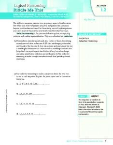
Before you continue the development of a formal proof as Exercise 1, let us illustrate the theorem with a Venn diagram. First we draw a circle for set G (Figure 5.1):

Figure 5.1 By the hypothesis F © G , we put the circle representing set F inside set G , as in Figure 5.2:

Figure 5.2


33

By hypothesis 2, E © F, we draw set E inside circle F, as in Figure 5.3. It is clear from the diagram, now, that E is inside G ; that is, the conclusion E © G is true.

Figure 5.3 EXERCISES 1. Fill in the underlined places in the following proof fragments. (a) 1. C - G 2. 0 9< +66 B - G À B • "# 3. __________

(_______;_______)

(b) 1. _______ 2. 0 9< +66 > - F À > - G 3. _______

(1ß 2; us. a )

(c) 1. ; - F 2. 0 9< +66 > - F À > - G 3. _______

(1ß 2; us. a )

(d) 1. & - W 2. 0 9< +66 B - W À B - X 3. ______

(1ß 2; us. a )

(e) 1. % - W 2. _________________ 3. % - X

(1ß 2; us. a )

(f) 1. B - W 2. _________________ 3. B - X

(1ß 2; us. a )

2. Prove Theorem 5.1. Stick exclusively to the step-discovery procedure.

34

The Basic Ideas of Mathematics, Teacher Edition © A.Wohlgemuth REVIEW EXERCISES 3. 1. Let B - V be arbitrary. . 7. B • ) 8. ______________________

(_____; pr. a )

4. Fill in the steps dictated by the rule for proving a 0 9< +66 statement (a)

8. 0 9< +66 B - E À & • B

(______; pr. a )

6. 0 9< +66 B - G À B - H

(______; pr. a )

(b)

Section 6

35

Using S< Statements Definition

For sets E and F, the union of E and F is the set E • F defined by E • F œ ÖB ± B - E 9< B - F×. The word “9 - • ± > • #!× G œ Ö> - • ± > • $!× E•F © G

Show:

k. E • F © G

The conclusion is of the form =/> © =/>. This top-level form regards E • F as a single set. From the form of the conclusion, we get the justification for Step k. Proof: Assume: E œ Ö> - • ± > • "!× F œ Ö> - • ± > • #!× G œ Ö> - • ± > • $!× Show:

E•F © G

k. E • F © G

(

; def. © )

By the definition of © , we get the following defining condition as Step k-1.

k-1. 0 9< +66 B - E • F À B - G k. E • F © G

(k-1; def. © )

At the top level, statement k-1 is a 0 9< +66 statement. Thus the rule for proving 0 9< +66 statements is the justification for Step k-1. This rule dictates Steps 1 and k-2.

1. Let B - E • F be arbitrary. . k-2. B - G

38

The Basic Ideas of Mathematics, Teacher Edition © A.Wohlgemuth k-1. 0 9< +66 B - E • F À B - G k. E • F © G

(1—k-2; pr. a ) (k-1; def. © )

At the top level, Statement k-2 is of the form /6/7/8> - =/>. The justification for this step is therefore the definition of the set.

1. Let B - E • F be arbitrary. . k-2. B - G k-1. 0 9< +66 B - E • F À B - G k. E • F © G

(

; def. G )

(1—k-2; pr. a ) (k-1; def. © )

Getting B - G as Step k-2 from the definition of G , means that the condition defining G (applied to B) must be Step k-3.

1. Let B - E • F be arbitrary. . k-3. B • $! k-2. B - G k-1. 0 9< +66 B - E • F À B - G k. E • F © G

(k-3; def. G ) (1—k-2; pr. a ) (k-1; def. © )

Step k-3 is of the form 8?7,/< • 8?7,/ - =/>. The definition of that set gives us Step 2. Since B is in the set, B must satisfy the defining condition.

1. Let B - E • F be arbitrary. 2. B - E 9< B - F

(1; def. • )

. k-3. B • $! k-2. B - G k-1. 0 9< +66 B - E • F À B - G k. E • F © G

(k-3; def. G ) (1—k-2; pr. a ) (k-1; def. © )

At the top level, Step 2 is an 9< statement. We are now in the position of wanting to use an 9< statement that we know is true (Step 2) to prove B • 30 (Step k-3). The rule for using 9< statements tells us just what to do.

Section 6: Using S< Statements

39

1. Let B - E • F be arbitrary. 2. B - E 9< B - F Case 1

(1; def. • )

3. B - E . j-1. B • $!

Case 2

j. B - F . k-4. B • $!

k-3. B • $!

(2—k-4; us. 9 - =/>. The reason for Step 4 is therefore the definition of that set.


(1; def. • )

3. B - E 4. B • "!

(3; def. E )

. j-1. B • $! Case 2

j. B - F . k-4. B • $!

k-3. B • $!

(2—k-4; us. 9 - • ± > • "!× F œ Ö> - • ± > • #!× G œ Ö> - • ± > • $!× Show:

E•F © G

40



Case 2

(1; def. • )

3. B - E 4. B • "!

(3; def. E )

5. "! • $!

(given)

6. B • $!

(4ß 5; Trans. • )

7. B - F 8. B • #!

(7; def. F )

9. #! • $!

(given)

10. B • $!

(8ß 9; Trans. - E: > - F 3. B - F

(1; def. © , exp.) (2, 2 1/2; us, a )

The effect of using the implicit definition rule is to remove from proofs some statements of a basic logic form, and to leave only more mathematical looking statements. Example 2: Recall the proof of Example 1 of Section 5:

Proof: Assume: O œ ÖB - • ± B • #!× N©O Show:

0 9< +66 + - N : + • #! 1. Let + - N be arbitrary. 2. 0 9< +66 B - N : B - O

(hyp.; def. © )

3. + - O

(1ß 2; us. a )

4. + • #! 5. 0 9< +66 + - N : + • #!

(3; def. O ) (1— 4; pr. a ) ¨

Steps 1, 2, and 3 are needed—if we use the explicit form of the definition of © :

Section 7: Implicit Defining Conditions

47


(hyp.; def. © )

3. + - O

(1ß 2; us. a )

By using the implicit definition rule, however, we can use the hypothesis (N © O ) and Step 1 (+ - N ) to infer + - O immediately—which we now renumber as Step 2: Proof: Assume: O œ ÖB - • ± B • #!× N©O 0 9< +66 + - N : + • #!

Show:

1. Let + - N be arbitrary. 2. + - O 3. + • #! 4. 0 9< +66 + - N : + • #!

(1, hyp.; def. © , imp.) (2; def. O ) (1— 3; pr. a ) ¨

Using the implicit definition rule tends to focus our attention on the mathematical objects we're talking about, and not on the logical form of statements about them. Our logic should become increasingly implicit (but well understood). Note that our proof style begins with completely explicit use of definitions, inference rules, and formal statements. We move to implicit use of the rules after some practice with the explicit use. The correct approach from a pedagogical viewpoint is to move from the explicit to the implicit—not vice versa. In any area where understanding is paramount, shortcuts should not be learned before one gets the lay of the land. Example 3: Recall the proof of Example 4 of Section 4: Proof: Assume: L œ ÖB - • ± B • "!× K œ ÖB - • ± B • #!× Show:

L©K 1. Let B - L be arbitrary. 2. B • "!

(1; def. L )

3. "! • #!

(given)

4. B • #!

(2ß 3; Trans. • )

5. B - K

(4; def. K )

6. 0 9< +66 B - L À B - K

(1— 5; pr. a )

7. L © K

(6; def. © ) ¨

The defining condition for L © K (Step 7) is explicitly written down as Step 6. If we were to use the implicit definition rule, we would not write the 0 9< +66 statement of Step 6 down in the

48

The Basic Ideas of Mathematics, Teacher Edition © A.Wohlgemuth proof. We would go through all the steps necessary to prove this 0 9< +66 statement, but we would consider these steps as proving the equivalent statement L © K instead of the 0 o< +66 statement. The 0 9< +66 statement becomes implicit: Proof: Assume: L œ ÖB - • ± B • "!× K œ ÖB - • ± B • #!× Show:

L©K 1. Let B - L be arbitrary. 2. B • "!

(1; def. L )

3. "! • #!

(given)

4. B • #!

(2ß 3; Trans. • )

5. B - K

(4; def. K )

6. L © K

(1—5; def. © , imp.) ¨

The implicit definition rule is involved when we provide counterexamples to statements about set containment. For example, consider the following statement, which we call a proposition, since, at this stage, we presumably don't know whether it is true or false. Proposition

If E and F are sets, then E • F © F . The hypotheses and conclusion are: Hypotheses: Eß F sets Conclusion:

E•F © F

In order to exhibit a counterexample, we need to know what it means for E • F © F to be false. By definition of containment, E • F © F means 0 9< +66 B - E • F À B - F. The negation of this is >2/= B - E • F =?-2 >2+> B Â F. This tells us what it means for the 0 9< +66 statement to be false. Finding such an B will show that the 0 9< +66 statement is false. Since we mentally identify the statement E • F © F with the 0 9< +66 statement, we consider that to exhibit sets E and F and an element B that make the 0 9< +66 statement false is to provide a counterexample to the assertion about set containment. For example: Proposition

If E and F are sets, then E • F © F . Counterexample 4: Hypotheses: Eß F sets Conclusion:

E•F © F

Let E œ Ö"× and F œ Ö#×. Then E • F œ Ö"ß #×. Also " - Ö"ß #× but " Â Ö#×, so that Ö"ß #× © Ö#× is false.

Section 7: Implicit Defining Conditions

49

EXERCISES 1. In each exercise below, first fill in the underlined place using the implicit definition rule. Then in the second, explicit version of the same proof fragment, fill in the “missing ” step with the explicit defining condition, and get the same conclusion as in the first steps. (a) 1. G © H 2. B - G 3. _________________

(1ß 2; def. © , imp.)

1. G © H 2. B - G 2 "# . _________________ 3. _________________

(1; def. © , exp.) (2ß 2 "# ;___________)

(b) 1. X © Y 2. _________________ 3. > - Y

(1ß 2; def. © , imp.)

1. X © Y 2. _________________ 2

" #.

_________________

3. > - Y

(1; def. © , exp.) (2ß 2 "# ;___________)

(c) 1. Let B - E be arb. 2. B - F 3. __________________

(1—2; def. © , imp.)

1. Let B - E be arb. 2. B - F 2

" #.

__________________

(1—2; ________)

3. __________________

(2 "# ; def. © , exp.)

2. Rewrite the proof of Theorem 5.1, using the implicit definition rule in as many places as you can. 3. Rewrite the proof of Theorem 6.1, using the implicit definition rule in as many places as you can.

50

The Basic Ideas of Mathematics, Teacher Edition © A.Wohlgemuth REVIEW EXERCISES 4. (a) 1. B - E 9< C - E Case 1

2. Assume B - E 3. ÞÞÞ 4. C - F

Case 2

5. ___________ 6. ÞÞÞ 7. ___________

8. ________________

(1—7; us. 9 - G 9< > - H 2. ____________

(1; def. • , exp.)

(d) 1. B - K • L 2. _______________ Case 1

(1; def. • , exp.)

3. ____________ 4. ÞÞÞ 5. ____________

Case 2

6. ____________ 7. ÞÞÞ 8. ____________

9. B • *

(2—8; us. 9 - E +8. B - E

(1ß 2; pr. & )

(c) 1. K œ L 2. _______________

(1; def. œ , exp.)

3. _______________

(2; us. & )

4. _______________

(2; us. & )

(d) 1. K œ L 2. ______

(1; def. œ , imp.)

3. ______

(1; def. œ , imp.)

(e) 1. _____ 2. _____ 3. K œ L

(1ß 2; def. œ , imp.)

2. Use the step-discovery procedure to fill in all the proof steps you can leading up to a proof of a proposition with the following hypothesis and conclusion: Assume: Kß L sets Show:

KœL

Give a counterexample to show that K œ L is not true for all sets K and L . 3. Prove Theorem 9.1. 4. Prove Theorem 9.2, and draw a Venn diagram that illustrates the theorem. 5. Let E , F , G , and H be sets. Prove or disprove the following propositions: (a) E © E • F. (b) If E © F and G © H, then E • G © F • H .

Section 9: Intersections; E8. Statements REVIEW EXERCISES 6. Write all the steps dictated by the rule for proving 9< statements that show Step k.

k. B Ÿ * 9< B - G

7. (a)

(_____; pr.9 Â G . 3. > - H 4. _______________

(b)

(1—3; ________)

4. Let > - G be arbitrary . 7. > - H 8. ________________

(4—7;________)

(c) 1. _______ 2. > - \ • ]

(1; def. • , imp.)

65

66


Section 10

67

Symmetry Theorem 10.1

For sets E and F, (a) E • F œ F • E (b) E • F œ F • E We will use the proof of Theorem 10.1a as motivation for a new inference rule that will enable us to abbreviate proofs considerably. The final version of the proof will employ this rule. You are to employ the same rule to prove part (b). Note that the inference rule you will use to prove part (b) is stated after Theorem 10.1. In general, you are allowed to use any rule stated in a section to prove any theorem in the section—regardless of the order in which the rule and theorem are stated. This won't violate the principle of orderly, logical development, since the rules don't depend on theorems for their validity. Proof: Assume: E,F sets Show:

E•F œ F•E

k-1. E • F © F • E +8. F • E © E • F k. E • F œ F • E

( ; pr. & ) (k-1; def. œ , exp.)

We have written the conclusion as Step k. This step is of the form =/> œ =/>, so we use the definition of equal sets to get Step k-1. Step k-1 is an +8. statement. The rule for proving +8. statements dictates two previous steps—which we write separately, since the two steps will have to be shown separately. Proof: Assume: E,F sets Show:

E•F œ F•E

. j. E • F © F • E . k-2. F • E © E • F k-1. E • F © F • E +8. F • E © E • F k. E • F œ F • E

(j, k-2 ; pr. & ) (k-1; def. œ , exp.)

68

The Basic Ideas of Mathematics, Teacher Edition © A.Wohlgemuth Note that the definition of intersection has not entered into the analysis yet. There are two steps (j and k-2) to establish. Further analysis leads to the following steps toward establishing Step j:

1. Let B - E • F be arbitrary . j-2. B - F • E j-1. 0 9< +66 B - E • F À B - F • E j. E • F © F • E

(1—j-2; pr. a ) (j-1; def. © )

The definition of intersection and the rules for proving and using +8. statements provide the missing steps:

1. Let B - E • F be arbitrary 2. B - E +8. B - F

(1; def. • , exp.)

3. B - E

(2; us. & )

4. B - F

(2; us. & )

5. B - F +8. B - E

(3ß 4; pr. & )

6. B - F • E

(5; def. • , exp.)

7. 0 9< +66 B - E • F À B - F • E

(1—6; pr. a )

8. E • F © F • E

(7; def. © , exp.)

We have established Step j (now Step 8), the first of the steps needed to prove the +8. statement in Step k-1. We now need to establish the second step, k-2: F • E © E • F. But notice that Step k-2 is just Step 8 with the roles of E and F reversed. Steps 9 through 16 are obtained by rewriting Steps 1 through 8 with the roles of E and F reversed:

1. Let B - E • F be arbitrary 2. B - E +8. B - F

(1; def. • , exp.)

3. B - E

(2; us. & )

4. B - F

(2; us. & )

5. B - F +8. B - E

(3ß 4; pr. & )

6. B - F • E

(5; def. • , exp.)

7. 0 9< +66 B - E • F À B - F • E

(1—6; pr. a )

8. E • F © F • E

(7; def. © , exp.)

9. Let B - F • E be arbitrary 10. B - F +8. B - E

(9; def. • , exp.)

11. B - F

(10; us. & )

12. B - E

(10; us. & )

13. B - E +8. B - F

(11ß 12; pr. & )

14. B - E • F

(13; def. • , exp.)

Section 10: Symmetry 15. 0 9< +66 B - F • E À B - E • F

(9—14; pr. a )

16. F • E © E • F

(15; def. © , exp.)

69

The complete proof is therefore: Proof of (a): Assume: E,F sets Show:

E•F œ F•E 1. Let B - E • F be arbitrary 2. B - E +8. B - F

(1; def. • , exp.)

3. B - E

(2; us. & )

4. B - F

(2; us. & )

5. B - F +8. B - E

(3ß 4; pr. & )

6. B - F • E

(5; def. • , exp.)

7. 0 9< +66 B - E • F À B - F • E

(1—6; pr. a )

8. E • F © F • E

(7; def. © , exp.)

9. Let B - F • E be arbitrary 10. B - F +8. B - E

(9; def. • , exp.)

11. B - F

(10; us. & )

12. B - E

(10; us. & )

13. B - E +8. B - F

(11ß 12; pr. & )

14. B - E • F

(13; def. • , exp.)

15. 0 9< +66 B - F • E À B - E • F

(9—14; pr. a )

16. F • E © E • F

(15; def. © , exp.)

17. E • F © F • E +8. F • E © E • F

(8ß 16 ; pr. & )

18. E • F œ F • E

(17; def. œ , exp.) ¨

Since Steps 9 through 16 are identical to Steps 1 through 8, except that the roles of E and F have been reversed, it is just a matter of uninformative busy work to write all the repetitive steps down. We will shortcut the process by replacing Steps 9 through 16 above with Step 9 below: Proof of (a): Assume: E,F sets Show:

E•F œ F•E 1. Let B - E • F be arbitrary 2. B - E +8. B - F

(1; def. • , exp.)

3. B - E

(2; us. & )

4. B - F

(2; us. & )

5. B - F +8. B - E

(3ß 4; pr. & )

6. B - F • E

(5; def. • , exp.)

70

The Basic Ideas of Mathematics, Teacher Edition © A.Wohlgemuth 7. 0 9< +66 B - E • F À B - F • E

(1—6; pr. a )

8. E • F © F • E

(7; def. © , exp.)

9. F • E © E • F

(1—8; symmetry in E and F)

10. E • F © F • E +8. F • E © E • F

(8ß 9 ; pr. & )

11. E • F œ F • E

(10; def. œ , exp.) ¨

The use of symmetry is formalized with the following rule, which we call an inference rule, although it would more properly be called a shortcut rule. Inference Rule Using Symmetry: If a sequence of steps establishes the statement dÐE,FÑ in a proof, and if the sequence of the steps is valid with the roles of E and F reversed, then the statement d ÐF,EÑ (d with E and F reversed) may be written as a proof step. Abbreviation: “sym. E & F”. Note that in using symmetry in E and F in going from Step 8 to 9 in the proof above, we are doing this: E•F © F•E Æ Æ Æ Æ F•E©E•F not this: E•F © F•E

F•E©E•F A statement cÐE,FÑ that we accept as true for the sake of argument is called a premise. Thus the hypotheses that we get by interpreting theorem statements are premises. We also call assumptions made within a proof premises. Statements valid under the latter kind of premise are written at the same indentation level as the premise, or as further indentations within that level. The principle behind the use of symmetry is that if d ÐE,FÑ follows from the premise c ÐE,FÑ, then d ÐF,EÑ follows from the premise c ÐF,EÑ. The reason is that “E” and “F” are just names which could just as easily be interchanged. In the proof above, the statement dÐE,FÑ (E • F © F • E) follows from an empty set of premises: the symbols “E” and “F” are named in the hypotheses, but there are no assumptions made about E and F. The empty set of premises is symmetric in E and F. The first set mentioned could be called “F” just as well as “E”. The statement d ÐF,EÑ (F • E © E • F) also follows from the hypotheses, and is at the same, highest indentation level—not dependent on any additional premises that are not symmetric in E and F. When a step justified by symmetry depends on no premises (and is therefore at the highest indentation level) we list in the justification the symmetric step and the block of steps used to establish it. For example, the justification (1—8; sym. E & F) for Step 9 in the proof above means that Step 9 is symmetric with Step 8 and that Steps 1 through 7 establish Step 8. More examples of this situation are given in Section 14. When a step justified by symmetry depends on symmetric premises, these premises are referred to in the justification. An example of this situation is given in the proof of Theorem 14.5. Note that in the proof above of Theorem 10.1a it would not be valid to use symmetry to interchange E and F in any of the indented steps 2 through 6, since these steps depend on the premise B - E • F, which is not symmetric in E and F (unless the assertion of the theorem is known in advance). Symmetry can safely be used as an effort saving rule, where you can see the validity of the steps that you are not writing down. You will never need to use symmetry to do proofs. In fact, if

Section 10: Symmetry

71

the use of symmetry is too handy, it should be suspect. Being symmetric with a true statement does not, in itself, make a statement true. Using the implicit definition rule can further shorten the proof. Step 2 gives the defining condition that is equivalent to the statement of Step 1. Rather than writing this +8. statement down as a step, we use it, implicitly, to get Steps 3 and 4. Similarly, Step 6 follows immediately from Steps 3 and 4, by the implicit use of the condition defining intersection. Also, if we use the definition of © implicitly as justification for Step 8, the 0 9< +66 statement of Step 7 need not be written as a step. If we use the definition of set equality implicitly as justification for Step 11, the +8. statement of Step 10 need not be written as a step. Thus we have the following, shortened proof: Proof of (a): Assume: E,F sets Show:

E•F œ F•E 1. Let B - E • F be arbitrary 2. B - E

(1; def. • , imp.)

3. B - F

(1; def. • , imp.)

4. B - F • E

(2ß 3; def. • , imp.)

5. E • F © F • E

(1—4; def. © , imp.)

6. F • E © E • F

(1—5; sym. E & F)

7. E • F œ F • E

(5ß 6; def. œ , imp.) ¨

Step 1, B - E • F, means B - E +8. B - F to us, since we know the definition of intersection. Therefore, to use B - E • F we use the implicit +8. statement, to infer Steps 2 and 3, but we think of this as using Step 1. Similarly, from Steps 2 and 3, we can infer the statement B - F +8. B - E, but we think of this as inferring Step 4, B - F • E. The rule for implicit use of definitions allows us not only to contract what we write down, but to contract our thought processes. Thus we ignore the obvious, and are better able to focus on more fruitful things. In the next section, we take up informal, narrative-style proofs where logic is implicit. The rules for proving and using +8. statements disappear when we write in paragraph style. The statement “B - E and B - F” in a paragraph proof could correspond to either the one step “k. B - E +8. B - F” or to the two steps “k. B - E” and “k+1. B - F”. Our formal rules for proving and using +8. make these two possibilities logically equivalent. While the +8. rules fade away, the effects of other rules, although no longer explicit, can still be detected as they provide a basis for the form of the logical arguments. EXERCISE 1. Prove Theorem 10.1b. Use symmetry.

72

The Basic Ideas of Mathematics, Teacher Edition © A.Wohlgemuth REVIEW EXERCISES 2. (a)

1. Assume > - G . 4. > - H 5. ________________

(1—4;________)

(b) 1. _____ 2. _____ 3. G œ H

(1ß 2; def. œ , imp.)

(c) 1. ____________ 2. > - \ • ]

(1; def. • , exp.)

(d) 1. G œ H

(e)

2. ______

(1; def. œ , imp.)

3. ______

(1; def. œ , imp.)

1. ___________ . 5. ___________ 6. > - \ • ]

(1—5; def. • , imp.)

(f) 1. G œ H 2. _______________

(1; def. œ , exp.)

3. _______________

(2; us. & )

4. _______________

(2; us. & )

(g) 1. _____________ 2. _____________ 3. > • ) +8. > - G

(1ß 2; pr. & )

(h) 1. > - G +8. > Ÿ ) 2. _____________

(1; us. & )

Section 11

73

Narrative Proofs Proofs in the mathematical literature don't follow the step-by-step form that our proofs have taken so far. Instead, they are written in narrative form using ordinary sentences and paragraphs. The primary function of such narrative proofs is to serve as a communication between writer and reader, whereas the step-by-step proofs we have considered so far are primarily logical verifications. In a narrative proof, the writer takes for granted a certain level of sophistication in the reader. Thus certain details can be left out, since it is presumed that the reader can easily supply them if they are needed. Generally, the higher the level of the mathematics, the more detail left out. Our rule for the implicit use of defining conditions produces proofs that are intermediate between narrative proofs and the step-by-step proofs with explicit logic. Logic is always implicit in narrative proofs. We will illustrate the formulation of narrative proofs as abbreviations of step-by-step proofs with implicit logic. Example 1: Consider the shortened version of the proof of Theorem 10.1a that used the implicit definition rule. Theorem 10.1

For sets E and F, (a) E • F œ F • E (b) E • F œ F • E

Proof of (a): Assume: E,F sets Show:

E•F œ F•E 1. Let B - E • F be arbitrary 2. B - E

(1; def. • , imp.)

3. B - F

(1; def. • , imp.)

4. B - F • E

(2ß 3; def. • , imp.)

5. E • F © F • E

(1—4; def. © , imp.)

6. F • E © E • F

(1—5; sym. E & F)

7. E • F œ F • E

(5ß 6; def. œ , imp.) ¨

A narrative proof begins with a sentence or two that cover the hypotheses and conclusion. This is merely good writing style: first you tell your reader what you are assuming, and then what you will show:

74


Proof of (a): We assume that E and F are any sets, and will show that E • F œ F • E. Next, we relate the steps that take us to the conclusion: Proof of (a): We assume that E and F are any sets, and will show that E • F œ F • E. Let B - E • F be arbitrary. Then B - E and B - F by the definition of • . From this we get B - F • E. Therefore E • F © F • E by the definition of © . F • E © E • F follows by symmetry, and from the last two assertions we get E • F œ F • E, by the definition of set equality. ¨ In a narrative proof, it isn't necessary to cite the justification for every step taken. Omit the justification when you think it will be clear to the reader. Don't be too repetitive. You should always, however, cite the hypotheses where these are used in the proof. The hypotheses are there because the theorem isn't true without them. It is a good idea therefore, to show where the hypotheses are needed in the proof. Example 2: Rewrite the proof of Theorem 8.2 as a narrative proof. Theorem 8.2

For sets E, F and G , if E © F 9< E © G then E © F • G . Proof: Assume: E,F,G sets E © F 9< E © G Show:

E©F•G 1. Let B - E be arbitrary 2. Assume B Â F 3. E © F 9< E © G

Case 1

4. Assume E © F

Case 2

6. Assume E © G

5. B - Fß # Step 2

(hyp.) (1ß 4; def. © , imp.)

7. B - G

(1ß 6; def. © , imp.)

8. B - G

(3—7; us. 92/8 > - P

(b)

(1—4; pr. Ê )

1. _____________ . 4. _____________ 5. 30 > - K, >2/8 > - L

(c)

(1—4; pr. Ê )

1. _____________ . 4. _____________ 5. 0 9< +66 > - K: > - L

(1—4; pr. a )

1. Assume > - E

(d)

. 4. > - F 5. __________________

(1—4; ________ )

1. Let > - E be arbitrary

(e)

. 4. > - F 5. __________________

(1—4; ________ )

(f) 3. + • ' . 5. 30 + • ', >2/8 + - F 6. ___________________

(3ß 5; us. Ê )

Section 14: Implications; Equivalence

99

(g) 2. + Ÿ ' . 5. ___________________ 6. , Ÿ '

(2ß 5; us. Ê )

(h) 1. __________________ 2. 30 > - K, >2/8 > - L 3. > - L

(1ß 2; us. Ê )

(i) 1. K © L 2. __________________ 3. L © N (j)

(1ß 2; us. Ê )

1. _____________ 2. _____________ 3. 30 E © F, >2/8 E © G

(1ß 2; pr. Ê )

(k) 1. c +8. d 2. 30 c , >2/8 e 3. ____________

(___________)

4. e

(___________)

(l) 1. ___________________ 2. ___________________

(1; pr. __________)

3. 30 B - F, >2/8 E © F

(2; Thm. 14.1: c 9< d Í 30 cc ,>2/8 d )

(m) 1. _____________ 2. B • & 9< E © F

(1; Thm. 14.1: c 9< d Í 30 cc ,>2/8 d ) .

2. Prove Corollary 14.2 3. Prove Theorem 14.4. 4. Give a proof of Theorem 10.1b (For sets E and F, E • F œ F • E) using Theorem 14.3, the rule for using equivalence (implicitly), and symmetry. 5. Prove Corollary 14.6. 6. Prove Theorem 14.7. 7. Prove Corollary 14.8. 8. Suppose that c , d , e, and f are formal language statements. Assume:

1. c 9< d 2. 30 c , >2/8 e 3. 30 d , >2/8 f

Show:

e 9< f

100


Section 15

101

Proof by Contradiction When mathematicians want to prove some statement c , they frequently assume the negation of c , and show that this leads to a contradiction. Such a proof by contradiction depends on the following axiom of logic, which formalizes the fact that a statement is either true or false—by definition. Axiom

For any statement c , c 9< cc is true. Suppose that we knew a sequence of steps that lead to a contradiction from the premise cc . For example, suppose that we know that B - G , and can show that B Â G follows from cc . The statement c is then proved as follows: 1. B - G 2. c 9< cc Case 1

3. c

Case 2

4. cc

(Ax.: c 9< cc )

. 6. B Â G # Step 1 7. c

(2—6; us. 92/8 d is true. If d is true, then this doesn't happen—so 30 c ß >2/8 d is true. Thus the two short proofs above make sense. We will capture these as EZ forms of the rule for proving if-then: Formats: pr. Ê EZ 1. cc k. 30 c ß >2/8 d

15

(1; pr. Ê EZ)

One can prove anything at all, including B • (, under the assumption B - E, since in a system [indented steps] with contradictions, anything can be shown to be true.

106

The Basic Ideas of Mathematics, Teacher Edition © A.Wohlgemuth pr. Ê EZ 1. d k. 30 c ß >2/8 d

Ð1; pr. Ê EZ)

If when applying the step-discovery procedure, you need to prove a statement of the form 30 c ß >2/8 d , the thing to do is to assume c and show d —unless cc or d happens to be a previously known step. In that case, merely conclude 30 c ß >2/8 d by the EZ form of the rule. This will avoid the need to assume something contrary to a known step. In mathematics, you may assume anything you like, without violating logic, since mathematics knows how to contain the results of such an assumption, without it infecting an entire argument. But this may make some people uncomfortable. In following the step-discovery procedure, you should only make those assumptions that are dictated by the analysis. Example 4: Let c be the statement ) • (, and d the statement ' • (Þ Then cc is true, so by the EZ form of the rule for proving 30 ->2/8 statements, 30 c ß >2/8 d is true. The converse, 30 d ß >2/8 c , is the statement 30 ' • (ß >2/8 ) • ( — and this statement is evidently false. It illustrates the only way for an implication to be false: namely, for the hypothesis to be true, and the conclusion false (see Theorem 15.3). Such is not the case for the statement 30 ) • (, >2/8 ' • ( — which is therefore a true statement. Such implications, with a false hypothesis, are called vacuously true. Theorem 15.3 and the arguments leading to the EZ forms of the rule for proving implications show why mathematicians accept such statements. Some people are quite uncomfortable with vacuously true statements—probably because the precise, mathematical meaning of an 30 ->2/8 statement does not exactly agree with their informal usage of “30 ->2/8”. Example 5: Consider the statement 30 B - Ö"ß #×ß >2/8 B - Ö"ß #ß $×. It is evidently true—with anyone's interpretation of 30 ->2/8. The converse is the statement 30 B - Ö"ß #ß $×ß >2/8 B - Ö"ß #×. Most users of informal mathematical language would consider this converse as false. What they mean by the statement is that “if B is an arbitrarily chosen element from the set Ö"ß #ß $×, then B is in the set Ö"ß #×”. In such a construction, B is called a free variable. We have not yet touched on free variables, and we would need to capture the same meaning with the formal statement 0 9< +66 B - • À 30 B - Ö"ß #ß $×ß >2/8 B - Ö"ß #× — and this formal statement is certainly false. For us, at this point, the statement 30 B - Ö"ß #ß $×ß >2/8 B - Ö"ß #× could not be made unless B were previously defined. And the truth of 30 B - Ö"ß #ß $×ß >2/8 B - Ö"ß #× would depend on the value of the previously defined B: if B were $, the implication would be false; if B were any other number (say, ", #, or "(), the implication would be true. Dealing with negations (89> statements) when using the step-discovery procedure There is no inference rule for either using or proving top-level negations. In order to deal with such statements we use either a proof by contradiction or axioms and theorems that involve equivalent statements. Example 6: Let E and F be any sets. Use the step-discovery procedure to find steps leading to a proof of cÐE © FÑ. Solution 1: 1. Assume E © F to get # 2. 0 9< +66 B - E À B - F

(1; def. © )

Section 15: Proof by Contradiction

107

. k-1. get # here k. cÐE © FÑ

(1—k-1; # )

In Solution 1, it now remains necessary to use the 0 9< +66 statement of Step 2 in order to obtain some contradiction. Solution 2: . . k-2Þ >2/= B - E =?-2 >2+> B Â F

(______; pr. b )

k-1. cÐ0 9< +66 B - E À B - FÑ

(k-2; Axiom: neg. a )

k. cÐE © FÑ

(k-1; def. © )

By definition of © , E © F is equivalent to 0 9< +66 B - E À B - F. By the axiom on page 22: if c is equivalent to d , then cc is equivalent to cd 16. We therefore find Step k-1 by substituting cÐ0 9< +66 B - E À B - FÑ for cÐE © FÑ. In the justification for Step k, we make explicit reference to the equivalence of the relation and its defining condition. The axiom stating the equivalence of the negations is used implicitly. We find Step k-2 by substituting a >2/= statement for the negation of a 0 9< +66 statement—these being equivalent by the axiom on page 15. It now remains necessary to prove the formal >2/= statement of Step k-2. The rule for doing this is introduced in Section 18. A proof by contradiction can be employed to use the negation of an element's being in a set. For example, suppose F œ ÖB - • ± B • "!×. If we knew > - • and > Â F, we would like to be able to infer that > • "! was false. One proof that from > - • and > Â F we can infer cÐ> • "!Ñ is as follows: 1. > Â F 2. Assume > • "! to get # 3. > - F, # Step 1 4. cÐ> • "!Ñ

(2; def. F ) (2—3; # )

Equivalently, > Â F is equivalent to cÐ> • "!Ñ, since > - F is equivalent to > • "! — by substitution, or by the axiom on page 22. Summary

Using set definitions: Suppose E œ ÖB ± c ÐBÑ× and > is any element of the universal set. From > - E we may infer c Ð>Ñ, and, conversely, from c Ð>Ñ we may infer > - EÞ Also from > Â E we may infer cÐc Ð>ÑÑ and from cÐc Ð>ÑÑ we may infer > Â E. Example 7: Define H œ ÖB - • ± B • %×. The definition of H tells us why Step 2 below follows from Step 1, and why Step 4 follows from Step 3. 1. + Â H 2. cÐ+ • %Ñ

(1; def. H )

3. cÐ, • %Ñ 4. , Â H 16

(3; def.H )

At our present stage, we could establish this axiom as an easy theorem obtained by substitution and our rule for proving equivalence.

108

The Basic Ideas of Mathematics, Teacher Edition © A.Wohlgemuth From our experience with the system of natural numbers, we know that cÐ+ • %Ñ is equivalent to % Ÿ +. This fact depends on an axiom (trichotomy) for the natural numbers that we will consider later. Solution 2 to Example 5 illustrates the following summarizing convention:

Summary

Using the definition of a relation: Suppose some relation has been defined. Then, if the relation holds, the defining conditi

on may be inferred. Conversely, if the defining condition holds, then the relation may be inferred. Also, if the negation of the relation holds, then the negation of the defining condition may be inferred, and conversely. Example 8: 1. cÐW © X Ñ 2. c 0 9< +66 B - W À B - X

(1; def. © )

Example 9: 1. B Â E • F 2. cÐB - E +8. B - FÑ

(1; def. • )

EXERCISES 1. (a) 1. G œ ÖB - • ± B • (× 2. C Â G 3. _________________

(1ß 2; def. G )

(b) 1. H œ ÖB ± c ÐBÑ× 2. C Â H 3. ___________

(1ß 2; ________)

4. D - H 5. ___________

(1ß 4; ________)

(c) 1. E © F 2. ____________

(1; __________)

(d) 1. cÐE © FÑ 2. ____________

(1; __________)

(e) 1. B Â E • F 2. ____________

(1; __________)

2. Prove that for any sets E and F, and any element B, if B Â E, then B Â E • F .

Section 15: Proof by Contradiction 3. Prove that for any sets E and F, and any element B, if B - E and B Â E • F, then B Â F. 4. Prove that for any sets E and F, and any element B, if B Â E 9< B Â F, then B Â E • F . 5. Prove Theorem 15.1. 6. Prove Theorem 15.2. REVIEW EXERCISES 8. (a) 1. _____________ . 4. _____________ 5. 30 D - E, >2/8 D - F

(1—4; pr. Ê )

(b) 1. Assume D - K . 4. D - L 5. __________________

(1—4; ________ )

(c) 1. Let D - K be arbitrary . 4. D - L 5. __________________

(1—4; ________ )

(d) 2. + ž ' . 5. ___________________ 6. , ž '

(2ß 5; us. Ê )

(e) 1. F © G 2. __________________ 3. G © H

(1ß 2; us. Ê )

109

110


Section 16

111

Investigation: Discovering Set Identities The axioms given in Section 13 presented the commutative and associative properties of addition and multiplication of the natural numbers. These properties also hold for the set operations of union and intersection—as was stated in Theorem 9.1 and Corollaries 14.6 and 14.8: Theorem 9.1

For sets E and F, (a) E • F œ F • E (b) E • F œ F • E

Corollary 15.6

For sets E, F, and G , ÐE • FÑ • G œ E • ÐF • GÑ.

Corollary 15.8

For sets E, F, and G , ÐE • FÑ • G œ E • ÐF • GÑ. The distributive property “if +ß ,ß - - •, then + † Ð, € -Ñ œ + † , € + † -” relates the two operations of addition and multiplication. It says in which way we can either multiply first and then add, or add first and then multiply. In this section we want to discover in what ways the set operations of intersection and union are related. In fact, we will also consider a third set operation, that of set difference.

Definition

For sets E and F, the complement of F in E (also called the difference) is the set E • F (read “E minus F ”) defined by: E • F œ ÖB l B - E +8. B Â F×. Example 1: (a) If E œ Ö#ß $ß %ß &× and F œ Ö%ß &ß 'ß (× , then E • F œ Ö#ß $× . (b) ÖB - • l B • "!× • ÖB - • l B • '× œ Ö'ß (ß )ß *×

The set E • F is pictured as the shaded area in the Venn diagram of Figure 16.1.

Figure 16.1 Before we seek relationships between set difference and the other set operations, union and intersection, we first ask if the commutative and associative properties hold for difference. In order

112

The Basic Ideas of Mathematics, Teacher Edition © A.Wohlgemuth to answer this question, we first consider whether E • ÐF • GÑ œ ÐE • FÑ • G holds, for example, for the sets in the following Venn diagram:

Figure 16.2 The validity of E • ÐF • GÑ œ ÐE • FÑ • G for the sets Eß F ß G above is checked as in the following example: Example 2: E

•

•

ÐF•GÑ

? œ

? œ

ÐE • FÑ

•

G

•

œ

Since the shaded area representing E • ÐF • GÑ is exactly the same as the shaded area representing ÐE • FÑ • G , we conclude that E • ÐF • GÑ œ ÐE • FÑ • G for the sets above. Notice, however, that there is a relationship that holds between the sets EßFß and G in the Venn diagram, namely, that G © F • E . Sets E and F such that E • F œ g are called disjoint. If also E • G œ g and F • G œ g , then the three sets EßFß and G are called mutually disjointÞ Three mutually disjoint sets EßFß and G are pictured in the following Venn diagram:

Figure 16.3

Section 16: Discovering Set Identities

113

The validity of E • ÐF • GÑ œ ÐE • FÑ • G for the sets Eß F ß G above is checked in the following example. Example 3: E

•

ÐF•GÑ

? œ

ÐE • FÑ

? œ

•

•

G

•

œ

Here again we see that E • ÐF • GÑ œ ÐE • FÑ • G — this time under the condition that the sets EßFß and G are mutually disjoint. If we wish to see whether E • ÐF • GÑ œ ÐE • FÑ • G is true for all sets, then we need to consider a Venn diagram in which there are no relations between that sets EßFß and G . In such a diagram, the sets are said to be in general position. The following diagram exhibits EßFß and G in general position.

Figure 16.% The validity of E • ÐF • GÑ œ ÐE • FÑ • G for the sets Eß F ß G above is checked in the following example. Example 4: E

•

•

ÐF•GÑ

? œ

? œ

Á

ÐE • FÑ

•

•

G

114

The Basic Ideas of Mathematics, Teacher Edition © A.Wohlgemuth From the diagrams above, we see that E • ÐF • GÑ œ ÐE • FÑ • G is not true for all sets EßFß and G . In particular, it is not true for those sets pictured in Example 4 .Thus the sets in Example 4 serve as a counterexample to the assertion: “For all sets EßFß and G , E • ÐF • GÑ œ ÐE • FÑ • G.” As an exercise, you can find sets of natural numbers that also serve as a counterexample. Example 2 leads us to believe that E • ÐF • GÑ œ ÐE • FÑ • G might be true for all sets that satisfy the hypothesis E © F • G . Thus we have the following conjecture: “For sets EßFß and G , if E © F • G , then E • ÐF • GÑ œ ÐE • FÑ • G .” We also suspect the following conjecture: “For mutually disjoint sets EßFß and G , E • ÐF • GÑ œ ÐE • FÑ • G.”

Investigation 1: Draw sets E and F in what you would consider to be general position. Using this diagram, show that E • F œ F • E is not true for all sets E and F. Thus, both the commutative and associative properties fail for the operation of set difference. Can you find some hypothesis under which E • F œ F • E is true? How many different conditions can you find that will insure that E • F œ F • E is true? (See the investigations in Section 20.) The set equations E • F œ F • E and ÐE • FÑ • G œ E • ÐF • GÑ, for example, are true for all sets EßFß and G . Such equations, true for all values of the variables, are called identities. The purpose of this section is to discover (and prove) set identities that relate the set operations of union, intersection, and difference—just as the distributive property for multiplication over addition relates these two operations on the natural numbers. Identities that you find to be true as a result of your investigations in this section can be labeled Theorem 16.1, 16.2, and so on. Investigation 2: By shading a diagram for sets EßFß and G in general position (Figure 16.4), obtain the Venn diagrams that represent the following sets—sets that are unions, intersections, and differences. UNIONS E F G E•F E•G F•G

INTERSECTIONS E F G E•F E•G F•G

DIFFERENCES E F G E•F E•G F•G F•E G•E G•F

Now find the sketches of the intersections of all the unions you have that involve all three sets EßFß and G . (For example, sketch E • ÐF • GÑ, because it is an intersection of unions, and because it involves EßFß and G ). Don't repeat symmetric situations. (For example, having sketched E • ÐF • GÑ, don't bother to sketch F • ÐE • GÑ—which is merely symmetric in E and FÑ. Label the diagrams with the sets that they represent. Use parentheses to remove ambiguities in your expressions. Then do the same thing to sketch the intersections of the differences. Then find the sketches of all the unions of the intersections and differences. Finally, sketch the differences of the intersections and unions. Example 5: You should have obtained the sketch shown in Figure 16.5 as an intersection of differences: ÐE • FÑ • ÐE • GÑ—or something symmetric to this expression.

Section 16: Discovering Set Identities

115

Figure 16.5

Investigation 3: Look through your sketches to find where the same shaded region is described by two or more set expressions. For each such region, make a list of the different ways the region can be described. In mathematics, to say + œ , always means that + and , are two names, or two representations, or two descriptions for exactly the same thing. If the same region of the Venn diagram can be described in two different ways, these two representations must be equal for the sets in the diagram. Set your two expressions for the shaded area equal to each other, to get a set equation. Since each of the two ways represents the same set in the Venn diagram, the equation must be true for the sets in the diagram. Conjecture that the equation is true for all sets E, F, and G . Prove this conjecture, or find a counterexample. Repeat the process for other regions. Proven conjectures can be called theorems. Some theorems that you can discover in this way are more important than the theorems in the text. The point of these investigations is to discover relationships between the operations of set union, intersection, and difference. For example, to find a relationship between union and intersection, look for a region that can be described as a union at the top-level, and also as an intersection at the top level. To find other relationships between the same two operations, look for other regions that can be so described. Example 6: The Venn diagrams for the sets ÐE • FÑ • G and ÐE • FÑ • ÐG • FÑ are symmetric:

ÐE • FÑ • G

ÐE • FÑ • ÐG • FÑ

If we interchange the roles of F and G in the right-hand expression and Venn diagram we get a Venn diagram that is exactly the same as the left hand diagram:

ÐE • FÑ • G

ÐE • GÑ • ÐF • GÑ

We therefore conjecture that for all sets EßFß and Gß ÐE • FÑ • G œ ÐE • GÑ • ÐF • GÑ.

116


Section 17

117

Axiom for Existence; Uniqueness The axioms of Section 13 don't give us any elements of •, they merely assert what must be true about any elements that there may be in •. The following axiom gives us an element in •, in terms of which all the elements of • can be defined. It is called an identity for multiplication. Existence of identity for multiplication: X 2/= D - • =?-2 >2+> Ð0 9< +66 + - • À D † + œ +Ñ

Axiom

The identity for multiplication is, of course, the number “one”. Before we give it its usual name, however, we prove, from the axioms, that there can't be more than one such identity. It is very important in mathematics not to use a single symbol to represent two different things. We want to use the symbol “1” to stand for the identity for multiplication, so we must show there is only one such identity. In this case, we say that the identity is unique. We have the following formal rule for proving uniqueness: Inference Rule Proving uniqueness: To prove that an element with property c is unique, assume two different names, say B" and B# , for an element or elements with property c , and then show B" œ B# . Abbreviation: “pr. x ” Format: pr. ! Assume: c ÐB" Ñ (read “B" has property c ” or “c holds for B" ”) cÐB# Ñ Show:

B" œ B#

In mathematics we always use the word “unique” in relation to some property: we say that an element is unique such that the property holds. By this we mean that there is only one element for which the property holds. For an identity D for multiplication, the property c ÐDÑ is: 0 9< +66 + - •: D † + œ + Theorem 17.1

There exists a unique D - • such that Ð0 9< +66 + - •: D † + œ +Ñ The phrase “there exists a unique” in Theorem 17.1 comprises two separate parts: existence and uniqueness. The statement of Theorem 17.1 is equivalent to the two assertions:

and

(1) >2/= D - • =?-2 >2+> Ð0 9< +66 + - •: D † + œ +Ñ (2) the element whose existence is given in (1) is unique.

In order to prove statements like the one in Theorem 17.1, we therefore need to do two things: (1) prove the existence statement, and (2) prove uniqueness. For Theorem 17.1, the existence part is an axiom, and doesn't need proof. The uniqueness part is proved using the rule for proving uniqueness.

118

The Basic Ideas of Mathematics, Teacher Edition © A.Wohlgemuth Proof: The existence part, there exists D - • such that Ð0 9< +66 + - •: D † + œ +Ñ, is a restatement of the axiom we assume. To prove the uniqueness part we have: Assume: D" , D# integers 1. 0 9< +66 + - •: D" † + œ + 2. 0 9< +66 + - •: D# † + œ + Show:

D" œ D#

1. D" † D# œ D#

(hyp. 1; us. a )

2. D# † D" œ D"

(hyp. 2; us. a )

3. D" † D# œ D"

(2; comm. † )

4. D" œ D#

(1,3; sub.) ¨

Step 3 comes from Step 2 by reversing D" and D# in the product D# † D" , by the axiom that gives the commutativity of multiplication. The steps in the proof of Theorem 17.1 can be written in terms of a more natural (less formal) proof style that involves a chain of equalities: +" œ +# œ +$ œ ÞÞÞ œ +8 , usually written vertically in proofs: +" œ +#

(reason that +" œ +# )

œ +$

(reason that +# œ +$ )

œ +8

(reason that +8 •" œ +8 )

. .

If we used such a chain, the steps in the preceding proof would be:

D" œ D# † D"

(D2 is † identity)

œ D" † D#

(comm. † )

œ D#

(D1 is † identity) ¨

We now know that there is only one multiplicative identity, and we give it its usual name “1”. The property asserting existence of an identity can then be rewritten using the symbol “1” and the commutative property: Axiom

Property of † identity: 0 9< +66 + - • À " † + œ + œ + † " It is very important, at this point, to distinguish between our imaginative idea of addition and the properties of addition given by the axioms. Through experiences with counting — one, two, three, four, five, ... — we learn to use numbers as adjectives, and to come to conclusions involving this use. For example, we see that 2 apples plus 3 apples gives 5 apples, 2 pears plus 3 pears gives 5 pears, and so on. From this experience with using numbers as adjectives, we come to an abstract understanding of numbers as nouns. We realize that # € $ œ & is a true statement about

Section 17: Axiom for Existence; Uniqueness

119

numbers, that is, about the nouns. All civilizations with written languages have had symbols (called numerals) for the numbers one, two, three, four, and so on. This understanding of the natural numbers as nouns is the most basic idea in mathematics. It is even more basic than the idea of proof. Nevertheless, it is important to remain faithful also to the idea of proof—where everything must follow either from definitions or from axioms relating undefined terms. We need to use statements such as # € $ œ & in proof steps. Justification of such an equation must follow from the definitions of the terms involved and the axioms relating undefined terms. It is not legitimate, in a proof step, to bring in an appeal to some physical situation—to claim, for example, that two apples “plus” three apples gives five apples. To do this would be to import an imaginative idea of addition that is not completely captured in the axioms. The natural numbers #ß $ß %ß & and so on, are defined in terms of the identity of multiplication, ", given by our axiom. Define the number # as " € "Þ The number 3 is defined as # € ". Similarly, define % œ $ € "ß & œ % € "ß ' œ & € "ß and so on. By the closure axiom, #ß $ß %ß and so on, are all natural numbers. The formal definitions agree exactly with our intuition. From the definitions of the natural numbers, come all the facts about them. For example, the following facts, used to create multiplication and addition tables, derive from the definitions: #€# œ # € Ð" € "Ñ

(def.#)

œ Ð# € "Ñ € "

(assoc. € )

œ$€"

(def. $)

œ%

(def. %)

$€# œ $ € Ð" € "Ñ

(def. #)

œ Ð$ € "Ñ € "

(assoc. € )

œ%€"

(def. %)

œ&

(def. &)

$€$ œ $ € Ð# € "Ñ

(def. $)

œ Ð$ € #Ñ € "Ñ

(assoc. € )

œ&€"

(previously shown add. fact: $ € # œ &)

œ'

(def. ')

#†# œ # † Ð" € "Ñ

(def. #)

œ#†"€#†"

(distr.)

œ#€#

(mult. id.)

œ%

(previously shown add. fact: # € # œ %)

#†$ œ Ð" € "Ñ † $

(def. #)

œ"†$€"†$

(dist.)

œ$€$

(mult. id.)

œ'

(previously shown add. fact: $ € $ œ ')

We will allow such facts about the natural numbers, given in the addition and multiplication tables, (or more extensive computations for large numbers) to be used as proof steps. For example, the statement ( € $ œ "! can be inserted in a proof with the justification “addition fact”.

120

The Basic Ideas of Mathematics, Teacher Edition © A.Wohlgemuth Example 1: 1. B € & œ + † ( € + † $ 2. B € & œ + † Ð( € $Ñ

(1; Ax.: For +ß ,ß - - ™, + † Ð, € -Ñ œ + † , € + † -Ñ

3. ( € $ œ "!

(addition fact)

4. B € & œ + † "!

(2ß 3; sub.)

Addition facts will frequently be used implicitly—as in the following example: Example 2: 1. B € & œ + † ( € + † $ 2. B € & œ + † Ð( € $Ñ

(1; Ax.: For +ß ,ß - - ™, + † Ð, € -Ñ œ + † , € + † -Ñ

3. B € & œ + † "!

(2; sub.)

EXERCISE 1. Define the numbers ', (, and ). (a) Show that $ € % œ (. (b) Show that # † % œ ).

Section 18

121

X 2/= Statements; Order We now get to the formal inference rules for using and proving >2/= statements. These were introduced informally on page 15 to explain the logic behind vacuously true statements, and on page 22 to introduce counterexamples. Recall the axioms on page 15 giving the negations of 0 9< +66 and >2/= statements: Axiom

J 9< +66 negation: cÐ0 9< +66 B - E À c ÐBÑÑ is equivalent to >2/= B - E =?-2 >2+> cc ÐBÑ.

Axiom

X 2/= negation: cÐ>2/= B - E =?-2 >2+> c ÐBÑÑ is equivalent to 0 9< +66 B - E : cc ÐBÑ. Example 1: For sets E and F, the relation E © F is equivalent to the statement 0 9< +66 B - E À B - F, by definitionÞ Thus cÐE © FÑ is equivalent to cÐ0 9< +66 B - E À B - FÑ by the axiom on page 22. In turn, cÐ0 9< +66 B - E À B - FÑ is equivalent to >2/= B - E =?-2 >2+> B Â F by the axiom above. Therefore, to find a counterexample to the assertion E © F, we informally showed this >2/= statement; that is, we defined an element B, showed that it was in E, and that it was not in F. We now formalize this as the basis for proving >2/= statements in proofs.

Inference Rule Proving >2/= statements: In order to prove the statement >2/= B - E =?-2 >2+> c ÐBÑ, define B in the proof steps. Then prove both B - E and c ÐBÑ for your B. Abbreviation: “pr. b ”. Format: pr. b

i.

j. B - E

k-1. cÐBÑ k. >2/= B - E =?-2 >2+> c ÐBÑ

(i, j, k-1; pr. b )

Inference Rule Using >2/= statements: From the statement >2/= B - E =?-2 >2+> c ÐBÑ we may infer both B - E and c ÐBÑ. Abbreviation: “ us. b ”. Format:

122

The Basic Ideas of Mathematics, Teacher Edition © A.Wohlgemuth us. b i. >2/= B - E =?-2 >2+> c ÐBÑ . j. B - E

(i; us. b )

. k. cÐBÑ

(i; us. b )

A >2/= statement (such as in Step i) is considered to define the symbol B, so that we may refer to it later in the proof (for example, in Steps j and k). In the first sections, we considered an order relation • on the set • as given, so that we could use it in numerical examples of sets. The transitive property of • was taken as an axiom, which applied the examples, but not to any of the theoretical development. It wasn't used to prove any of the theorems about sets. We now give a formal definition of the relation • , and prove the transitive property from its definition and the axioms for addition and multiplication. Definition

For +ß , - •, define + is less than b (written + • ,) iff >2/= B - • =?-2 >2+> , œ + € B. The proof of the following theorem depends on the rules for proving and using >2/= statements:

Theorem 18.1

Transitivity of • : For natural numbers +ß ,ß and -, if + • , and , • -, then + • -. Proof: Assume: +ß ,ß - - ™ 1. + • , 2. , • Show:

+•-

. Þ k-1. >2/= B - • =?-2 >2+> - œ + € B k. + • -

(k-1; def. • )

We now need to prove the >2/= statement of Step k-1. Steps i, j, and k-2 are dictated by the rule for proving such statements.

. i. . j. B - • Þ k-2. - œ + € B k-1. >2/= B - • =?-2 >2+> - œ + € B k. + • -

(k-1; def. • )

Section 18: X 2/= Statements; Order

123

The bottom-up analysis of the step-discovery procedure has identified just what we need to do: define B, and show that B - • and - œ + € B are true about the B we define. We can continue no further from the bottom up, so we use one of the hypotheses:

1. >2/= B - • =?-2 >2+> , œ + € B

( hyp. 1: + • , )

. i. . j. B - • Þ k-2. - œ + € B k-1. >2/= B - • =?-2 >2+> - œ + € B k. + • -

(k-1; def. • )

The B that we are given in Step 1 might not be the same as the B we need to define in Step i, so we need to use another letter as the variable in Step 1. The steps we have above are all correct and logical, but if we continue from the development above, we can't define B in Step i, because it has already been defined by the >2/= statement of Step 1. So we use a letter other than B in Step 1.

1. >2/= C - • =?-2 >2+> , œ + € y

( hyp. 1: + • , )

. i. . j. B - • Þ k-2. - œ + € B k-1. >2/= B - • =?-2 >2+> - œ + € B k. + • -

(k-1; def. • )

The rule for using >2/= statements gives us Steps 2 and 3:

1. >2/= C - • =?-2 >2+> , œ + € y

( hyp. 1: + • , )

2. C - •

(1; us.b )

3. , œ + € y

(1; us.b )

. i. . j. B - • Þ k-2. - œ + € B k-1. >2/= B - • =?-2 >2+> - œ + € B k. + • -

(k-1; def. • )

124

The Basic Ideas of Mathematics, Teacher Edition © A.Wohlgemuth From the second hypothesis we get Steps 4, 5, and 6:

1. >2/= C - • =?-2 >2+> , œ + € C

( hyp. 1: + • , )

2. C - •

(1; us.b )

3. , œ + € C

(1; us.b )

4. >2/= D - • =?-2 >2+> - œ , € D

( hyp. 2: , • - )

5. D - •

(4; us.b )

6. - œ , € D

(4; us.b )

. i. . j. B - • Þ k-2. - œ + € B k-1. >2/= B - • =?-2 >2+> - œ + € B k. + • -

(k-1; def. • )

The step-discovery procedure has left us with (1) a clear definition of our task: define B and show B - • and - œ + € B for our B, and (2) the things we have to work with to define B: +ß ,ß and - from the hypotheses, and C and D, which have been defined in the proof steps. Since - œ , € D and , œ + € C, we can substitute + € C for , in the first equation to get: œ,€D œ Ð+ € CÑ € D œ + € ÐC € DÑ We can define B to be C € D. This is done with the statement “Let B œ C € D ”. We will use the word “let” in formal proofs in only this way; that is, to define a new symbol in terms of previously defined symbols (analogous to an assignment statement in computer science).

1. >2/= C - • =?-2 >2+> , œ + € C

( hyp. 1: + • , )

2. C - •

(1; us.b )

3. , œ + € C

(1; us.b )

4. >2/= D - • =?-2 >2+> - œ , € D

( hyp. 2: , • - )

5. D - •

(4; us.b )

6. - œ , € D

(4; us.b )

7. Let B œ C € D 8. B - •

(2, 5, 7; ax.: If :ß ; - •ß then : € ; - •)

9. - œ Ð+ € CÑ € D

(3, 6; sub.)

10. - œ + € ÐC € DÑ

(9; assoc. € )

11. - œ + € B

(7, 10; sub.)

12. >2/= B - • =?-2 >2+> - œ + € B

(7, 8, 11; pr.b )

13. + • -

(12; def. • ) ¨


125

The proof can be shortened with the following rule: Inference Rule Using >2/= implicitly: We may refer to either of the statements B - E or c ÐBÑ within a proof statement >2/= B - E =?-2 >2+> c ÐBÑ that is known to be true. That is, we need not rewrite these as proof steps. Using this rule allows us to use the formal statements C - • and , œ + € C within the >2/= statement of Step 1 — without rewriting these down as proof steps. Similarly, D - • and - œ , € D can be used right from within Step 4. This allows us to contract the proof:

1. >2/= C - • =?-2 >2+> , œ + € C

( hyp. 1: + • , )

2. >2/= D - • =?-2 >2+> - œ , € D

( hyp. 2: , • - )

3. Let B œ C € D 4. B - •

(1, 2, 3; ax.: If :ß ; - •ß then : € ; - •)

5. - œ Ð+ € CÑ € D

(1, 2; sub.)

6. - œ + € ÐC € DÑ

(5; assoc. € )

7. - œ + € B

(3, 6; sub.)

8. >2/= B - • =?-2 >2+> - œ + € B

(3, 4, 7; pr.b )

9. + • -

(8; def. • ) ¨

Note that the rule for implicit use of >2/= statements allows us to work from inside a >2/= statement, and not only at the top level. It is therefore an exception to the way we work with statements. In effect, we are able to interpret the >2/= statement informally. The >2/= statement of Step 8 need not be written as a proof step, if we use the definition of • implicitly:

1. >2/= C - • =?-2 >2+> , œ + € C

( hyp. 1: + • , )

2. >2/= D - • =?-2 >2+> - œ , € D

( hyp. 2: , • - )

3. Let B œ C € D 4. B - •

(1, 2, 3; ax.: • closed under € )

5. - œ Ð+ € CÑ € D

(1, 2; sub.)

6. - œ + € ÐC € DÑ

(5; assoc. € )

7. - œ + € B

(3, 6; sub.)

8. + • -

(3, 4, 7; def. • ) ¨

To justify Step 8, we need to refer to all the steps needed to prove the implicit >2/= statement: Step 3, where B is defined, and Steps 4 and 7 which state the needed properties of B. We can't use the definition of • implicitly in using the hypotheses, since the >2/= statements of Steps 1 and 2 are needed to define the elements C and D for subsequent use in the proof. We can, however, abbreviate the proof further by writing it as a narrative proof:

126


Narrative proof: Assume + • , and , • - for +ß ,ß - - •. We will show + • -Þ Since + • ,, there exists C - • such that , œ + € C, and since , • -, there exists D - • such that - œ , € DÞ Then - œ , € D œ Ð+ € CÑ € D œ + € ÐC € DÑ. Let B œ C € D. Then B - •, since • is closed under € . Also - œ + € B, so that + • - by definition of • . ¨

Definition

For integers + and ,, define + Ÿ , (which is read “+ is less than or equal to ,”) iff + • , 9< + œ , .

Theorem 18.2

Transitivity of Ÿ : For +ß ,ß - - ™, if + Ÿ , and , Ÿ -, then + Ÿ -. Proof: Exercise 3. Facts such as $ • ' were considered as “given” for use in the first sections. Here these facts about the natural numbers and the relation • can be shown from the definition of • and previously shown addition facts, which follow from the definition of the elements in •. Example 1: In order to show $ • ', we need to prove >2/= B - • =?-2 >2+> ' œ $ € BÞ Define B œ $. Then ' œ $ € B œ $ € $, by one of the previously shown addition facts. From now on, we will follow statements such as $ • ' in proofs with the abbreviated justification “(def. • )”. We will no longer assume that these are “given”. They follow (easily) from the definition of • — as in Example 1. For natural numbers + and ,, we define the relation + ž ,, read “+ is greater than ,”, to mean the same as , • +. We use “+ is greater than ,” rather than “, is less than +” if we wish + rather than , to be the subject of our sentence. Mathematically, + ž , and , • + mean exactly the same thing. In order that we need not refer to informal ideas in a formal proof, we need the following formal definition:

Definition

For integers + and ,, define + ž , iff , • +.

Theorem 18.3

Transitivity of ž : For Bß Cß D - •, if B ž C and C ž D, then B ž D. Proof: Exercises 4 and 5. EXERCISES 1. Write all the steps dictated by the rule for proving >2/= statements. (a)

k. >2/= > - W =?-2 >2+> > • ") (b)

k. >2/= B - E • F


127

2. The following proof fragments use the explicit version of the rule for using >2/= statements. Rewrite abbreviated versions of these proof fragments that use the inference rule for using >2/= statements implicitly. (a) 1. >2/= B - E =?-2 >2+> B • ( 2. B - E

(1; us. b )

3. E © G

(hyp.)

4. B - G

(2ß 3; def. © , imp.)

(b) 1. >2/= B - E =?-2 >2+> B - F 2. B - E

(1; us. b )

3. B - F

(1; us. b )

4. B - E • F

(2ß 3; def. • , imp.)

3. Prove Theorem 18.2. 4. Follow the step-discovery procedure to prove Theorem 18.3. 5. Use Theorem 18.1 to prove Theorem 18.3. Note that using previously shown theorems in a proof abbreviates the proof, since it makes those steps unnecessary that were used to show the previous theorem. Note also that using previously shown theorems can do no more than this. Anything that can be proved using a theorem can be proved by a direct appeal to definitions and axioms— although the latter process may be so lengthy as to be impractical. By using theorems, it is also not necessary to repeat any creative processes use in the discovery of their proofs; that is, by using theorems, we need not reinvent the (perhaps centuries of) mathematics that led to their proofs.

128


Section 19

129

Trichotomy It might seem that the axioms we have so far would be enough to tell us everything we need to know about •. This is not the case. In fact, we can't even prove that " is not equal to # from these axioms. The way that mathematicians show that such a proof is impossible is to find or invent a system in which all the axioms are true, but where " œ #. The system need not be intuitive; it only needs to be logically consistent. (In fact, if " œ # in the system, it will probably be counterintuitive to most people.) Before we give an example in which " œ #, we give a familiar example of a set on which we can define the operation of addition. Example 1: Suppose G is the set Ö"ß #ß $ß %ß &ß 'ß (ß )ß *ß "!ß ""ß "#×. Define addition on this set by the way you would add hours on the face of a clock. That is, * hours past ) o'clock is & o'clock: we add * and ) to get "(, and then subtract "# to get & . Thus * € ) œ &. In Exercise 6, you are asked to pick examples of numbers in G to illustrate the commutative and associative properties of addition.

Example 2: Suppose R is the set Ö"×. Define addition and multiplication on this set by the rules "€"œ" "†"œ" The set Ö"× together with the operations defined above satisfies all the axioms for • that we have so far; that is, if we replace • with R in all the axiomsß the axioms can be shown to be true statements. The properties all reduce to the equation " œ " (Exercise 7). If the number # were defined as " € " œ # for the system R of Example 2 (just as it is for •), then since " € " œ " in R , we would have " œ #. It similarly follows that # œ $ œ %, and so on. Also, the equation " € " œ " shows that >2/= B - R =?-2 >2+> " œ " € B. This means that " • ". Of course " • # also, because # œ ". The following axiom for the natural numbers prevents " • # and " œ # from both being true in • — as they are in R of Example 2. Axiom

Trichotomy: For any +ß , - •, exactly one of the following holds: (a) + • , (b) + œ , (c) , • + The informal phrase “exactly one of the following holds” in the trichotomy axiom means: (1) the formal statement Ð+ • ,Ñ 9< Ð+ œ ,Ñ 9< Ð, • +Ñ holds, and (2) if any of (a), (b), or (c) is taken as a hypothesis, then the negation of either of the others can be taken as a conclusion.

130

The Basic Ideas of Mathematics, Teacher Edition © A.Wohlgemuth The equation " € " œ # in the natural numbers • shows that >2/= B - • =?-2 >2+> # œ " € B. This means that " • #. By the trichotomy axiom above, then, we can't have " œ #. Also, since # € " œ $ in •ß >2/= B - • =?-2 >2+> $ œ # € B. This means that # • $. By trichotomy, then, # Á $. From " • # and # • $, we get " • $, by transitivity—and therefore " Á $, by trichotomy. Continuing in this manner, we see that each newly defined natural number is greater than and distinct from all the previously defined natural numbers. This gives us the well-known ordering of the natural numbers: " • # • $ • % • & • ÞÞÞ Further, no number in this list is equal to any other number in the list. You knew this by counting. We wanted to show that it follows from the axioms. Not much can be done with equations in the natural numbers. Being able to work with and solve equations is the major reason for the creation of the larger number systems. There are a few operations with equations that can be illustrated in the natural numbers. One of these is the fact that we can add the same number to each side of an equation—as in the following example: Example 3: Suppose that B - • and that we know that $B € # œ "( is a true statement (equation) about B. Then the fact that we can add % to each side of this equation is justified as in the following steps: 1. $B € # œ "(

(hyp.)

2. "( € % œ "( € %

(identity)

3. ($B € #Ñ € % œ "( € %

(1, 2; sub.)

Step 2 is an identity and needs no real justification. It will be acceptable to merely note the fact. The net effect of these steps is to add the number % to each side of the equation in Step 1. We don't wish to go through this complex procedure and its logic—which involves writing down an identity—every time we want to add the same number to each side of an equation. Consequently, we'll make up a theorem that allows us to merely add the same number to each side of an equation. The proof of the theorem will be the same as the derivation of Step 3 from Steps 1 and 2 above. That is, the theorem will merely be a generalization of the steps above. Theorem 19.1

If + œ , is an equation between natural numbers + and ,, and - is any natural number, then (a) + € - œ , € (b) + † - œ , † Proof of part (a): Assume: +ß ,ß - - • +œ, Show:

+€- œ ,€-

1. + € - œ + € -

(identity)

2. + € - œ , € -

(1, hyp.; sub.) ¨

Proof of part (b): Exercise 1. In applying this theorem, we don't quote the theorem or the theorem number. We merely state what number was added to each side of the equation:

Section 19: Trichotomy

131

Example 4: 6. % € B œ # † B 7. Ð% € BÑ € $ œ Ð# † BÑ € $

(6; add $ )

Example 5: 6. % € B œ # † B 7. Ð% € BÑ † & œ Ð# † BÑ † & Theorem 19.2

(6; mult. by & )

If B • C for Bß C - •, and if D - •, then (a) B € D • C € D (b) B † D • C † D Proof: Exercise 2. Theorem 19.1 has a converse that can be proved using the trichotomy axiom:

Theorem 19.3

Suppose +ß ,ß - - •. (a) If + € - œ , € -, then + œ ,. (b) If + † - œ , † -, then + œ ,. Proof of part (a): Assume: +ß ,ß - - • +€- œ ,€Show:

+œ,

1. Ð+ • ,Ñ 9< Ð+ œ ,Ñ 9< Ð, • +Ñ

(axiom: trichotomy)

Case 1 2. + • ,Þ 3. + € - • , € -

(2; Thm. 19.2a)

4. cÐ+ € - œ , € -Ñ # hyp.

(3; trichotomy)

Case 2 5. + œ , Case 3 6. , • + 7. cÐ, € - œ + € -Ñ # hyp. 8. + œ ,

(2—4; sym.) (1—7; us. 92/= - - • =?-2 >2+> + œ ,-. The customary notation for saying , divides + is , ± +. The statement , ± + is also expressed by saying “, is a factor of +” or “+ is a multiple of ,”. The formal statement >2/= - - • =?-2 >2+> + œ ,of the definition above can also be phrased + œ ,- 0 9< =97/ - - • Statements of either form may be called either >2/= statements or 0 9< =97/ statements. Example 2: 1. $ ± + 2. + œ $- 0 9< =97/ - - •

(1; definition of “divides”)

By the definition of divides, $ ± + is equivalent to + œ $- 0 9< =97/ - - •. Thus the statement of the relationship $ ± + in Step 1 can be replaced by its defining condition + œ $- 0 9< =97/ - - •, giving Step 2. Example 3: 1. + œ *- 0 9< =97/ - - • 2. * ± +

(1; definition of “divides”)

By the definition of divides, * ± + is equivalent to + œ *- 0 9< =97/ - - •. Thus the statement of the defining condition + œ *- 0 9< =97/ - - • in Step 1 can be replaced by the defined relation * ± +, to get Step 2. “Definition of divides” in justifications is abbreviated “def. ± ”. Example 4: 1. ____________ 2. >2/= D - • =?-2 >2+> B œ CD

(1; def. ± )

134


Solution: 1. C ± B 2. >2/= D - • =?-2 >2+> B œ CD Theorem 20.1

(1; def. ± )

Let +, ,, - - •. If , ± + and , ± - then , ± Ð+ € -Ñ. Proof: Exercise 1.

Theorem 20.2

Let +, ,, - - •. If , ± +, then , ± +-. Proof: Exercise 2

Theorem 20.3

Let +, ,, - - •. If + ± , and , ± -, then + ± -. Proof: Exercise 3. A >2/= statement can be used to give a formal definition of the empty set. Let ” be the universal set; that is, all sets that we consider will have elements from ”. Then we have the following definition:

Definition

A set W is /7:>C (written W œ gÑ iff cÐ>2/= B - ” =?-2 >2+> B - WÑ. We have used the formal phrase >2/= B - ” =?-2 >2+> B - W in this definition, since it is in the general form >2/= B - E =?-2 >2+> c ÐBÑ. From a statement >2/= B - ” =?-2 >2+> B - W in some proof, we could infer both B - ” and B - W , by the rule above. All elements must come from our universal set, however, so there is no need to clutter proof steps with assertions like B - ”—or to worry about it at all. For this reason, we will use the abbreviated statement >2/= B - W ,17 instead of the statement >2/= B - ” =?-2 >2+> B - W . The rules for proving and using the abbreviated statement are exactly the same as the rules for proving and using the longer version, except that we omit explicitly mentioning that elements are in the universal set. With this convention we have the following restatement if the definition:

Definition

A set W is /7:>C (written W œ gÑ iff cÐ>2/= B - WÑ. A proof of the following theorem illustrates the rules or proving and using >2/= statements, as they apply to the shortened statements.

Theorem 20.4

17

For sets E, F, and G , if E © F, and F • G œ g, then E • G œ g

The negation of the statement >2/= B - W is the statement 0 9< +66 B - ” À B Â W . That is, when we form the negation of >2/= B - W , we must realize that it is an abbreviation of >2/= B - ” =?-2 >2+> B - W.

Section 20: Divisibility; Formal Iff Statements

135

Proof: Assume: E, F, G sets E©F F•G œg Show:

E•G œg

k-1. c(>2/= B - E • G ) k. E • G œ g

(

; def. g)

In order to establish Step k-1, we assume the contrary: Proof: Assume: E, F, G sets E©F F•G œ g Show:

E•G œ g 1. Assume >2/= B - E • G to get # 2. B - E • G

(1; us. b )

3. B - E

(2; def. • )

4. B - F

(3, hyp.; def. © )

5. B - G

(2; def. • )

6. B - F • G

(4ß 5; def. • )

7. >2/= B - F • G

(1ß 6; pr. b )

8. c(>2/= B - F • G ) # 7.

(hyp.; def. g)

9. c(>2/= B - E • G ) 10. E • G œ g

(1—8; # ) (9; def. g) ¨

The >2/= statement of Step 1 defines the symbol B, and the rule for using >2/= statements allows us to infer B - E • G about this B. We can omit Step 2 by using the rule implicitly. In general, the rule for proving the statement >2/= B - E =?-2 >2+> c ÐBÑ states that we must define B and show both that B is in E and that c ÐBÑ is true about B. Thus to prove Step 7, >2/= B - F • G , we need to define B and show B - F • G . Step 7 is justified by (1,6; pr. b ), since B is defined in Step 1 (by the >2/= statement) and shown to be in F • G in Step 6. If we use the definition of the empty set implicitly, we need not write down Step 9. That is, assuming (Step 1) that there is something in E • G , and then obtaining a contradiction proves that E • G is empty—by the definition of the empty set:

136


1. Assume >2/= B - E • G to get # 2. B - E

(1; def. • )

3. B - F

(2, hyp.; def. © )

4. B - G

(1; def. • )

5. B - F • G

(3ß 4; def. • )

6. >2/= B - F • G

(1ß 5; pr. b )

7. c(>2/= B - F • G ), # 6.

(hyp.; def. g)

8. E • G œ g

(1—7; def. g)

We can remove the step (6) with justification “pr. b ” by considering the statement >2/= B - F • G to be the defining condition for F • G Á g —which is the negation of one hypothesis. That is, we know that a statement and its defining condition are equivalent, so by the axiom “If c Í d , then cc Í cd ” we have that the negation of the statement is equivalent to the negation of the defining condition. By the extension of our implicit definition rule to apply to the negations of defining conditions, we can use the definition of the empty set implicitly to get a contradiction in the block of steps 1 through 7. That is, we think of >2/= B - F • G as the condition defining F • G Á g. To prove F • G Á g , therefore, we prove its defining condition >2/= B - F • G , but we don't write the defining condition down:

1. Assume >2/= B - E • G to get # 2. B - E

(1; def. • )

3. B - F

(2, hyp.; def. © )

4. B - G

(3; def. • )

5. B - F • G

(3ß 4; def. • )

6. F • G Á g, # hyp.

(1ß 5; def. g)

7. E • G œ g

(1—6; def. g) ¨

It's not possible to remove the formal >2/= statement of Step 1 from the proof, since this statement serves to define B. The proof of Theorem 20.4 illustrates how to handle expressions involving the empty set. In general, the way to prove \ œ g for some set \ , is to show that \ satisfies the property defining the empty set. Then \ œ g by definition of the empty set. Similarly, in order to use the information from a known equation ] œ g, use the fact that ] has the property defining the empty set; that is, ] is empty. The equation \ œ g has the form =/> œ =/>, so, by definition of set equality, it is equivalent to \ © g +8. g © \. Each of these expressions of set containment is equivalent to a 0 9< +66 statement. The 0 9< +66 statements will be vacuously true, and to prove such a statement we avoid using the rule for proving 0 9< +66 statements, which involves the assumption of a set being nonempty. (See the discussion on page 15.) Our proofs will not be effective communications if they contain vacuously true statements and assumptions that are contrary to known facts. Consequently, we use the definition of the empty set, to prove or use equations of the type \ œ g. The abbreviated proof, which uses implicit logic, can be rewritten as a narrative proof:

Section 20: Divisibility; Formal Iff Statements

137

Narrative Proof: Assume for sets EßFß and G that E © F and that F • G œ g. We show that E • G œ gÞ Thus assume there exists B - E • G in order to get a contradiction. Then B - E by the definition of intersection, so that by hypothesis B - F. Also, B - G by the definition of intersection, from which we get B - F • G —which contradicts the hypothesis. Consequently, E • G œ gÞ ¨ Consider The Venn diagram of Figure 20.1, which represents the hypotheses of Theorem 20.4.

Figure 20.1 In the diagram, we have drawn E © F and F • G œ g. (Recall that such sets F and G are called disjoint.) It is easy to see from he diagram that E and G must also be disjoint. While it is safe to infer set relationships from appropriately drawn Venn diagrams, it is not always safe to draw inferences from diagrams. The rule is that a diagram can be considered as part of a proof, provided that inferences drawn from the diagram can be confirmed, if necessary, by a step-by-step verification. With this understanding about the validity of using diagrams, proofs that depend on diagrams can be considered as a further step in the process of writing increasingly informal proofs. We have seen the following four types of proof, in order of increasing sophistication: (1) step-bystep proofs with explicit logic (formal inference rules explicitly expressed), (2) step-by-step proofs with implicit logic, (3) narrative-style proofs, and (4) proofs using inferences drawn from diagrams. Investigation 4: In Section 16, we conjectured that E • ÐF • GÑ œ ÐE • FÑ • G is true under either the hypothesis E © F • G or the hypothesis that EßFß and G are mutually disjoint. Verify both of these conjectures. In Section 16, you found conjectures about set identities by considering Venn diagrams for sets drawn in general position. Repeat Investigations 2 and 3 of Section 16—now, however, with some Venn diagrams for sets EßFß and G that exhibit some relationship; that is, are not in general position. This will lead to conjectures about set relationships that hold under certain hypotheses. The six types of basic, formal mathematical statements—>2/=ß 0 9< +66ß 30 ->2/8ß +8.ß 9—make up the language in which mathematics is expressed. Formal “iff” statements are defined in terms of 30 ->2/8 and +8. statements. Iff statements provide a formal analog to informal statements of equivalence. Recall that the informal idea of equivalence is used in definitions. Example 5: The relation of “subset” was defined as follows: For sets E and F, E © F iff 0 9< +66 B - E À B - F.

138

The Basic Ideas of Mathematics, Teacher Edition © A.Wohlgemuth The relationship E © F between E and F is equivalent, by definition, to the defining condition 0 9< +66 B - E À B - F.

Definition

The statement c 30 +8. 986C 30 d is defined to be the same as Ð30 c , >2/8 d Ñ +8. Ð30 d , >2/8 c Ñ. “M 0 +8. 986C 30 ” is also written “iff ”. In order to prove a statement c iff d we would prove Ð30 c , >2/8 d Ñ +8. Ð30 d , >2/8 c Ñ. This top-level +8. statement is proved in two parts, first we prove 30 c , >2/8 d , and then we prove 30 d , >2/8 c . These two parts are exactly what we do to show that c is equivalent to d . It is possible to speak informally about formal statements; that is, informal statements may contain formal statements. The reverse is not possible, however; that is, formal statements cannot contain informal ones. The formal iff is needed to get the idea of equivalence inside formal statements.

Theorem 20.5

For sets E and F, E œ F if and only if 0 9< +66 B - ”: B - E iff B - F. Proof: Exercise 6.

Theorem 20.6

For sets E and F: (a) E © F iff E • F œ E (b) E © F iff E • F œ F Proof: Exercise 7.

Investigation 5: The statement “if c , then d ” can be expressed by saying that c is a sufficient condition for d — or that d is a necessary condition for c . The statement “c iff d ” can be expressed by saying that c is a necessary and sufficient for d . In Investigation 1, you were asked if you could find some hypothesis under which E • F œ F • E was true—that is, could you find a sufficient condition on E and F for E • F œ F • E to be true? Is your sufficient condition also necessary? That is, have you found a necessary and sufficient condition for E • F œ F • E? Which of your hypotheses (sufficient conditions) from Investigation 4 are also necessary?

EXERCISES 1. Prove Theorem 20.1. 2. Prove Theorem 20.2. 3. Prove Theorem 20.3. 4. Prove that the statements >2/= B - E =?-2 >2+> B - F and >2/= B - E • F are equivalent. 5. Suppose that EßFß and G are sets, that E © F, and that E • G Á g. Prove that B • G Á g . 6. Prove Theorem 20.5. 7. Prove Theorem 20.6.

Section 21

139

The Integers In order to provide instructive examples of the functions in the following sections, we need to extend the system • of natural numbers to include zero and negative numbers. The extended number system is called the set of integers and is denoted by ™. The fact that ™ contains all the natural numbers already defined is recorded as our first axiom for the integers: Axiom

• © ™. The following axioms are the same as axioms that hold for •. Since these axioms hold for all elements in ™, they must hold for elements in the subset • of ™. It is therefore no longer necessary to retain these separately as axioms for •. We say that these properties of elements in • are now inherited from properties in ™.

Axiom

Commutativity of addition: If +ß , - ™, then + € , œ , € +.

Axiom

Associativity of addition: If +ß ,ß - - ™, then + € Ð, € -Ñ œ Ð+ € ,Ñ € -.

Axiom

Commutativity of multiplication: If +ß , - ™, then + † , œ , † +.

Axiom

Associativity of multiplication: If +ß ,ß - - ™, then + † Ð, † -Ñ œ Ð+ † ,Ñ † -.

Axiom

Distributivity: If +ß ,ß - - ™, then + † Ð, € -Ñ œ + † , € + † -. The following axioms for ™ are analogous to those for •:

Axiom

Closure under addition: If +ß , - ™, then + € , - ™.

Axiom

Closure under multiplication: If +ß , - ™, then + † , - ™. If we add two natural numbers, the result is another natural number. This fact doesn't follow from the axiom above, which tells us only that the sum will be some integer. That is, the fact that the natural numbers are closed under addition is not inherited from the axioms above for ™. We must therefore list it in addition to the axioms above. Thus we need to carry forward the following axioms for •:

Axiom

Closure of the subset • under addition: If +ß , - •, then + € , - •.

Axiom

Closure of the subset • under multiplication: If +ß , - •, then + † , - •. Since the element " that acts as an identity of multiplication for • is a member of the set •, and since • © ™, we have that " is an integer. The next axiom asserts that " acts as an identity of multiplication for all of ™—not only for the subset •.

Axiom

Identity for multiplication: J 9< +66 + - ™ À " † + œ + † " œ +.

140

The Basic Ideas of Mathematics, Teacher Edition © A.Wohlgemuth The next axiom for ™ asserts the existence of an identity for addition—something which • lacks, but which is included in the larger system ™.

Axiom

Identity for addition: X 2/= D - ™ =?-2 >2+> ÐD € + œ + € D œ + 0 9< +66 + - ™ÑÞ The identity for addition can be shown to be unique—exactly as the identity for multiplication was shown to be unique in Section 17. We can therefore give it its usual name !, and reword the axiom above:

Axiom

Identity for addition: ! € + œ + € ! œ + 0 9< +66 + - ™Þ

Theorem 21.1

! Â •Þ Proof: ! € ! œ !, so if ! - •, then ! • ! by definition of • — which would contradict trichotomy in •. Therefore ! Â •. ¨ The point of enlarging • is to include additive inverses. For example, the additive inverse of ( is denoted by -(. The integer -( has the property that when we add it to ( we get ! (the additive identity). The next axiom asserts that every integer has an additive inverse:

Axiom

Existence of an additive inverse: For each + - ™: >2/= + € , œ , € + œ !.18

Theorem 21.2

For each + - ™, there exists a unique , - ™ such that + € , œ !Þ

,-™

=?-2 >2+>

Proof: Exercise 1. The unique element , such that + € , œ ! (given by Theorem 21.2) is called “negative +” and is denoted by “-+”. Thus + € -+ œ !, and, by commutativity, -+ € + œ !. The operation of subtraction can be defined for elements of ™ in terms of additive inverses. Definition

For integers + and ,, define the integer + minus , (written + • , ) to be + plus the negative of ,. That is, + • , œ + € -,. The definition above defines subtraction for all integers, including the natural numbers. However, we already have a definition of subtraction for natural numbers, given on page 132. We must therefore show that the two definitions are equivalent. This follows from the next theorem.

Theorem 21.3

For any integers + and ,, + € -, œ B iff + œ , € B. Proof: Exercise 2.

18 The axiom is given informally—with hypotheses + - ™, and conclusion >2/= , - ™ =?-2 >2+> + € , œ , € + œ !. There is nothing to be gained by giving this axiom formally as a top-level 0 9< +66 statement. The reason for our formality is to guide in the step-discovery procedure, but an axiom doesn't need to be proved.

Section 21: The Integers

141

Investigation 6 Find theorems for the integers that are analogous to Theorems 19.1 and 19.3. If some statements that you get by replacing “natural number” with “integer” are not true, provide counterexamples. In the sequel, we will freely use these (true) theorems extended to the integers. Part (a) of the next theorem asserts that for any integer +, the inverse of the inverse of + is + itself; that is, -Ð-+Ñ œ +. The proof uses Theorem 21.2, which asserts the uniqueness of an inverse, and the following inference rule for using uniqueness: Inference Rule Using uniqueness: If we know that there is a unique element with property c , then from the facts c ÐB" Ñ and c ÐB# Ñ we can infer B" œ B# . Abbreviation: “ us. x ”. Example 1: 1. + € B œ ! 2. + € C œ ! 3. there exists a unique , - ™ such that + € , œ !

(Thm. 21.2)

4. B œ C

(1, 2, 3; us. ! )

By using the rule above implicitly, we need not cite it as justification for a step. Instead, we cite the theorem that asserts uniqueness, as in Example 2:

Example 2: 1. + € B œ ! 2. + € C œ ! 3. B œ C

Theorem 21.4

(1, 2; Thm. 21.2: For each + - ™, there exists a unique , - ™ such that + € , œ !)

For each +ß , - ™: (a) -Ð-+Ñ œ +. (b) ! † + œ ! (c) Ð-"Ñ † + œ -+ (d) -+ € -, œ -Ð+ € ,Ñ The proof of part (a) depends on the fact that -Ð-+Ñ is (by definition) the inverse of -+, and + is also an inverse of -+: Proof of (a): Assume: + an integer Show:

-Ð-+Ñ œ +

1. + € -+ œ !

(def. inverse)

2. -+ € + œ !

(1; comm. € )

3. -+ € -Ð-+Ñ œ !

(def. inverse)

4. + œ -Ð-+Ñ

(2, 3; Thm. 21.2: For each - - ™, there exists a unique , - ™ such that - € , œ !) ¨

142

The Basic Ideas of Mathematics, Teacher Edition © A.Wohlgemuth Proof of (b): Assume: + an integer Show:

!†+œ!

1. ! † + œ ! † +

(identity)

2. Ð! € !Ñ † + œ ! † +

(1; sub. ! is identity)

3. ! † + € ! † + œ ! † +

(2; dist.)

4. Ò! † + € ! † +Ó € -Ð! † +Ñ œ ! † + € -Ð! † +Ñ

(3; add -Ð! † +Ñ )

5. ! † + € Ò! † + € -Ð! † +ÑÓ œ ! † + € -Ð! † +Ñ

(4; assoc. € )

6. ! † + € ! œ !

(5; € inv. )

7. ! † + œ !

(6; € identity) ¨

Proof of (c) and (d): Exercises 2 and 3. It is a simple matter to extend the definition of order from • to all of ™: Definition

For +ß , - ™, + is said to be less than , (written + • ,) iff , œ + € B 0 9< =97/ B - •Þ Thus the integer + is less than the integer , iff we can add some natural number to , to obtain +. This definition clearly extends and does not conflict with the definition of order on • already given on page 122. The condition >2/= B - • =?-2 >2+> , œ + € B is logically equivalent to the condition , • + - •, as the following steps show: 1. >2/= B - • =?-2 >2+> , œ + € B 2. B - •

(1; us.b)

3. , œ + € B

(1: us.b)

4. -+ € , œ -+ € Ð+ € BÑ

(3; add -+ )

5. , € -+ œ Ð-+ € +Ñ € B

(4; comm. & assoc. + )

6. , • + œ ! € B

(5; def. sub. & inv.)

7. , • + œ B

(6; ! is € id.)

8. , • + - •

(2ß 7; sub.)

By reversing Steps 1 through 8 above and adjusting the justifications somewhat, we can prove that if we assume , • + - •, then we can show >2/= B - • =?-2 >2+> , œ + € B. The two conditions are therefore equivalent. This result is not important enough for us to call it a theorem, so we merely offer it as an alternate form for the definition of “ • ”: Definition

For +ß , - ™, define + • , iff , • + - •. Either form of the definition can be used to prove the parts of the following theorem.

Section 21: The Integers

Theorem 21.5

143

For all +ß , - ™: (a) ! • + iff + - • (b) -+ • ! iff + - • (c) + • ! iff -+ - • (d) + • , iff -, • -+ Proof: Exercise 5. Elements D - ™ such that D ž ! are called positive integers. By Theorem 21.5, a positive integer is just a natural number. Elements D - ™ such that D • ! are called negative integers

Axiom

Trichotomy for ™: For any +ß , - ™, exactly one of the following holds: (a) + • , (b) + œ , (c) , • + The trichotomy axiom for •, given on page 129, is clearly a consequence of this axiom. If we take , in the axiom to be zero, we see that every nonzero integer is either positive or negative and that no integer can be both positive and negative. Theorem 21.5 is therefore the basis for the ordering of the integers: ÞÞÞ -% • -$ • -# • -" • ! • " • # • $ • % ÞÞÞ Example 3: $ • ' (def. • ), so -' • -$ (Thm. 21.5d)

Theorem 21.6

For any + - ™, exactly one of the following holds: (a) + - • (b) + œ ! (c) -+ - • Proof: Exercise 6. Rules for adding, subtracting, and multiplying negative integers are based on theorems that we now consider.

Theorem 21.7

For all +ß , - ™: (a) Ð-+Ñ † , œ + † Ð-,Ñ œ -Ð+ † ,Ñ (b) Ð-+Ñ † Ð-,Ñ œ + † , Consider the statement Ð-+Ñ † , œ -Ð+ † ,Ñ which is part of (a). -Ð+ † ,Ñ is, by definition, the inverse of + † ,. In order to show Ð-+Ñ † , œ -Ð+ † ,Ñ, we show that Ð-+Ñ † , is also an inverse of + † ,, and then use the uniqueness of an additive inverse to conclude Ð-+Ñ † , œ -Ð+ † ,Ñ. In order to simplify our notation, we will write the product + † , as +,, that is, either the dot “ † ” (with numerals) or juxtaposition (with letters) will be used to denote a product.

144


Proof of part of (a): We assume +,, - ™ and show Ð-+Ñ, œ -+,. 1. +, € Ð-+Ñ, œ Ð+ € -+Ñ,

(dist.)

2. +, € Ð-+Ñ, œ ! † ,

(1; € inv.)

3. +, € Ð-+Ñ, œ !

(2; Thm. 21.4b: For each - - ™ À ! † - œ - )

4. Ð-+Ñ, is an inverse of +,

(3; def. inv.)

5. -+, is an inverse of +,

(notation for inv.)

6. Ð-+Ñ, œ -+,

(4,5; Thm. 21.0: uniqueness of € inverse) ¨

The remaining part of (a), +Ð-,Ñ œ -+,, and part (b) are exercises. Theorem 21.7 is true for any integers + and ,, not necessarily positive integers. If we take + and , to be positive integers, however, then -+ and -, are negative integers, and part (b) of the theorem states the fact, familiar from school computation, that a negative times a negative is positive: (neg.) † (neg.) œ (pos.). It is difficult to justify the rule (neg.) † (neg.) œ (pos.) to students acquainted only with descriptive mathematics and rules for computation. From our viewpoint, however, we see that the rule is a logical consequence of the axioms. If every integer has an additive inverse, and if the commutative, associative, and other axiomatic properties of the integers are to hold, then (neg.) † (neg.) œ (pos.) must hold also. From part (a) of this theorem, we get the rules (pos.) † (neg.) œ (neg.) and (neg.) † (pos.) œ (neg.). Of course, the rule (pos.) † (pos.) œ (pos.) comes from the closure of • under multiplication. Example 1: 1. Ð-&Ñ † Ð-%Ñ œ ____

(mult. fact)

Solution: 1. Ð-&Ñ † Ð-%Ñ œ #!

(mult. fact)

Theorem 21.7b and the previously accepted multiplication fact & † % œ #! give us the solution to Example 1. We will use Theorem 21.7b implicitly when justifying facts such as the one in Example 1—thus enlarging our multiplication facts to include multiplication by positive and negative integers. Theorem 21.8

For all +ß , - ™: (a) + € -, œ -Ð, • +Ñ (b) , € -+ œ , • + Proof: Part (b) is merely a restatement of the definition of subtraction. In order to prove part (a), assume that + and , are arbitrary integers. Then -Ð, • +Ñ œ -Ð, € -+Ñ

(def. subtr.)

œ Ð-"Ñ † Ð, € • +Ñ

(Thm. 21.4c )

œ Ð-"Ñ † , € Ð-"Ñ † Ð • +Ñ

(dist.)

Section 21: The Integers œ -, € Ð-"Ñ † Ð • +Ñ

(Thm. 21.4c )

œ -, € " † +

(Thm. 21.7b )

œ -, € +

(mult. id.)

œ + € -,

(comm. € )

145

¨ Theorem 21.8 applies to any integers + and , whatever—not only to natural numbers. If we apply the theorem to natural numbers + and ,, however, with + • ,, we get the following rule for adding integers of opposite sign. (Positive integers are said to have “positive sign”, and negative integers to have “negative sign”.) In order to add two integers of opposite sign, subtract the smaller from the larger, ignoring the signs of the integers. Then take the sign of the larger. Example 2: To add ( and -"!, ignore the signs of the numbers and observe ( • "!Þ Subtract the smaller from the larger: "! • ( œ $, using the subtraction facts for the natural numbers. Then assign the remainder $ a negative sign: ( € -"! œ -$. Equivalently, by Theorem 21.8a: ( € -"! œ -Ð"! • (Ñ. Example 3: To add ( and -&, ignore the signs of the numbers and observe & • (Þ Subtract the smaller from the larger: ( • & œ #, using the subtraction facts for the natural numbers. Then assign the remainder # a positive sign: ( € -& œ #. Equivalently, by Theorem 21.8b: ( € -& œ Ð( • &Ñ. Since a positive integer is just a natural number, to add two integers of positive sign, we use the addition facts (see page 119) for the natural numbers—which follow from the definitions of the numbers. To add two integers of negative sign, we use Theorem 21.4d: for +ß , - ™: -+ € -, œ -Ð+ € ,Ñ. Example 4: -( € -& œ -Ð( € &Ñ œ -"#. Subtraction of integers reduces to some kind of addition, by the rule that subtracting an integer is equivalent to adding the inverse of the integer. Example 5: The expression -( • -& involves subtracting a negative 5 from a negative 7. This is equivalent to adding the inverse of -& to the negative 7. Since, by Theorem 21.4a (-Ð-+Ñ œ +), the inverse of -& is &, we see that -( • -& is equivalent to -( € &, which by Theorem 21.8a is -( € & œ -Ð( • &Ñ œ -#Þ Symbolically: -( • -& œ -( € -Ð-&Ñ œ -( € & œ -Ð( • &Ñ œ -#. The following theorems provide a basis for the operations of adding, subtracting, or multiplying both sides of an inequality by the same number—in order to solve the inequality.

146


Theorem 21.9

For all +ß ,ß - - ™: (a) if + • ,, then + € - • , € (b) if + • , and - ž !, then +- • ,(c) if + • , and - • !, then +- ž ,Proof: Exercise 10.

Corollary 21.10 For all +ß ,ß - - ™: (a) if + Ÿ ,, then + € - Ÿ , € (b) if + Ÿ , and - ž !, then +- Ÿ ,(c) if + Ÿ , and - • !, then +- ž ,- (where +- ž ,- is defined by +- ž ,- 9< +- œ ,-) Proof: Exercise 11. EXERCISES 1. Prove Theorem 21.2. 2. Prove Theorem 21.3. 3. Prove Theorem 21.4c. Since -+ is the inverse of +, the equation here asserts that Ð-"Ñ † + is the inverse of +. This can be shown by adding Ð-"Ñ † + to + to get !, and then using the uniqueness of the additive inverse. By Theorem 21.4b and distributivity, we have ! œ ! † + œ Ð" € -"Ñ † + œ " † + € Ð-"Ñ † + œ + € Ð-"Ñ † +. Write this out as a formal step-by-step proof. 4. Prove Theorem 21.4d. Show that -+ € -, is an inverse of + € , by adding it to + € , to get !, and then use the uniqueness of the inverse. 5. Prove Theorem 21.5. 6. Prove Theorem 21.6. 7. Prove the following lemma: if B € + œ + or + € B œ + is true for any integers B and +, then B œ !. If B € + œ + is true for all + - ™, then B must be an identity for addition, and so must be zero by the uniqueness of such an identity. The content of the assertion you are to prove is that in order to have B œ !, we need not know B € + œ + for all + - ™ — only for one + - ™. This + may be B itself. Thus, by the lemma we may conclude B œ ! from B € B œ B. Use this lemma to write a proof of Theorem 21.4b that is shorter than the proof in the text. 8. Prove for all integers + and ,, +Ð-,Ñ œ -+, (the remaining part of Theorem 21.7a). 9. Prove Theorem 21.7b. 10. Prove Theorem 21.9. 11. Prove Corollary 21.10.

Section 22

147

Functions; Composition We have considered the mathematical idea of a set. Although this term was not formally defined, a particular set could be defined by our giving a rule (itself an undefined term) for deciding which elements are in the particular set and which are not. Another fundamental idea in mathematics is the idea of a function. Informally, a function is a rule of correspondence between two sets: a function 0 from a nonempty set E to a set F is a rule that associates to each element B of E a uniquely determined element, denoted 0 ÐBÑ, of F. 0 ÐBÑ is called the image of B under 0 . You can think of f as “sending” or “mapping” B in E to 0 ÐBÑ in F. Thus to know a particular function 0 from E to F, you must know a rule for getting 0 ÐBÑ in F given any B in E. The set E is called the domain of 0 , and F is called the codomain of 0 . The fact that 0 is a function from E to F is written 0 À E Ä F. Our format for defining a specific function will be to give (1) the function name together with the domain and codomain, (2) the rule that specifies what the function does to each element in the domain, and (3) a “for all elements in the domain” clause. A formal, set-theoretic definition of function is given in Section 25. Example 1: Define 0 À ™ Ä • by 0 ÐBÑ œ B# € $ 0 9< +66 B - ™. Then, for example, 0 Ð"Ñ œ "# € $ œ %, 0 Ð#Ñ œ (, 0 Ð!Ñ œ $, 0 Ð-"Ñ œ %, and so on. Example 2: Define 1À • Ä • by 1ÐBÑ œ 1 0 9< +66 B - •. Then, for example, 1Ð"Ñ œ 1ß 1Ð#Ñ œ ", and so on. Example 3: Define 2À • Ä • by 2ÐBÑ œ B € " 0 9< +66 B - •. Then, for example, 2Ð"Ñ œ Ð#Ñ, 2Ð#Ñ œ $, 2Ð$Ñ œ %, and so on. Example 4:

Define 5À • Ä • by 5ÐBÑ œ œ

" #

if B is odd . if B is even

Then, for example, 5Ð"Ñ œ ", 5Ð#Ñ œ #, 5Ð$Ñ œ ", 5Ð%Ñ œ #, and so on. Example 5: Define 0 À ™ Ä ™ by 0 ÐBÑ œ B. Then, for example, 0 Ð"Ñ œ ", 0 Ð#Ñ œ #, 0 Ð-"Ñ œ -", and so on. Note that the rules in Examples 1, 2, 3, and 5 for specifying the function are given by formulas but that the rule in Example 4 also specifies a function. Such a function is sometimes called conditionally defined. In all definitions, the 0 9< +66 quantification is optional since it is implied when the domain is specified. To use information in the definition of a function, use the (perhaps implicit) 0 9< +66 statement. The rule that defines a function is sometimes given by listing the images of the elements in the domain.

148


Example 6: Let E œ Ö+ß ,ß -ß . × and F œ Ö"ß #ß $ ×. Define 0 À E Ä F by 0 Ð+Ñ œ ",0 Ð,Ñ œ $, 0 Ð-Ñ œ $, and 0 Ð.Ñ œ ". (Sometimes arrows are used to give the same information: + Ä ", , Ä $, - Ä $, . Ä ".) It is sometimes helpful to diagram a function with its domain and codomain. For example, 0 À E Ä F is pictured as in Figure 1.

Figure 1 Definition

Let 0 À E Ä F. Define the set 0 ÐEÑ œ Ö, - F l , œ 0 ÐBÑ 0 9< =97/ B - E ×. 0 ÐEÑ is called the range of 0 . Example 7: Let 0 À • Ä • be given by the rule 0 ÐBÑ œ $B € ". 0 Ð"Ñ œ % 0 Ð#Ñ œ ( 0 Ð•Ñ œ Ö%ß (ß "!ß "$ß "'ß ... × The range of 0 À E Ä F is diagrammed in Figure 2.

Figure 2 Definition

Let 0 À E Ä F, 1À F Ä G . Define 1 ‰0 À E Ä G by 1 ‰0 Ð+Ñ œ 1Ð0 Ð+ÑÑ 0 9< +66 + - E. 1 ‰0 is a new function, called the composition of 1 with 0 , that has the effect of first applying 0 to an element in E and then applying 1 to the result. Note that for this to make sense, the range of 0 must be contained in the domain of 1. For simplicity, we take the codomain of 0 to be the domain of 1.

Section 22: Functions; Composition

149

Example 8: Let 0 À ™ Ä ™ be given by 0 ÐBÑ œ B • " and 1À ™ Ä ™ be given by 1ÐCÑ œ C# € #. Then 1 ‰0 À ™ Ä ™ is given by 1 ‰0 ÐBÑ œ 1Ð0 ÐBÑÑ œ 1ÐB • "Ñ œ ÐB • "Ñ# € #. Also 0 ‰ 1À ™ Ä ™ is given by 0 ‰ 1ÐCÑ œ 0 Ð1ÐCÑÑ œ 0 ÐC# € #Ñ œ ÐC# € #Ñ • " œ C# € ". Composition of functions 0 À E Ä F and 1À F Ä G is diagrammed in Figure 3.

Figure 3 In Example 8 we used the variable B describing 0 to also describe 1 ‰0 , since in 1 ‰0 we first apply 0 . Similarly, C describes both 1 and 0 ‰1. Although this was done to illustrate the way in which functions are composed, it is important to understand functions as rules. Composition of functions should therefore be viewed as a rule and not merely as the substitution of variables. The variables are only local variables needed to describe the rules. In the following example, doing without the aid of using different variables to describe 0 and 1 forces us to think of the functions as rules. Example 9: Let 0 À ™ Ä ™ be given by 0 ÐBÑ œ B# • & 0 9< +66 B - ™ and 1À ™ Ä ™ be given by 1ÐBÑ œ $B € # 0 9< +66 B - ™. (a) 1 ‰0 ÐBÑ œ (b) 0 ‰ 1ÐBÑ œ Solution: (a) 1 ‰0 ÐBÑ œ $ÐB# • &Ñ € # 0 9< +66 B - ™ (b) 0 ‰ 1ÐBÑ œ Ð$B € #Ñ# • & 0 9< +66 B - ™ Example 10: Let 0 À Ö"ß #ß $ß %× Ä Ö+ß ,ß -× be given by " Ä +, # Ä ,, $ Ä ,, % Ä -. Let 1À Ö+ß ,ß -× Ä ÖB,C,D× be defined by + Ä B, , Ä C, - Ä D . Then 1 ‰0 À Ö", #, $, %× Ä ÖB, C, z× is defined by " Ä B, # Ä C, $ Ä C, % Ä D. There is no function 0 ‰ 1 defined, since the domain of 0 is not the codomain of 119.

19

In defining 1‰0 we have used the usual definition of composition, where the domain of 1 is equal to the codomain of 0 . This definition will keep notation simple in future theorems, with no real loss of generality. Alternate definitions sometimes require only that the range of 0 be a subset of the domain of 1. The codomain of any such 0 can easily be redefined to be the domain of 1.

150

The Basic Ideas of Mathematics, Teacher Edition © A.Wohlgemuth Our next theorem asserts the associativity of composition, but first we need the idea of equal functions.

Definition

Two functions 0 À E Ä F and 1À E Ä F are said to be equal (written 0 œ 1) provided that 0 9< +66 B - E À 0 ÐBÑ œ 1ÐBÑ. Note that for 0 and 1 to be equal they must have the same domain and codomain (the context for definition). The definition just given states that functions are equal if the rules defining them yield the same value when applied to each element of their domain. The idea of equality asserts that the expressions on the left and right of the equal sign are just two names for exactly the same object. The reason we need definitions for equal sets and equal functions is that the ideas of set and function are themselves undefined. Therefore “sameness” needs to be defined in these cases.

Theorem 22.1:

Let 0 À E Ä F, 1À F Ä G , and 2À G Ä H. Then Ð2‰1Ñ‰0 œ 2‰Ð1‰0 Ñ. Note that at the top level, the conclusion is the statement that two functions are equal: Ð2‰1Ñ‰0 œ 2‰Ð1‰0 Ñ. By the definition of equality, we need to show two things in order to prove the theorem: (1) Ð2‰1Ñ‰0 and 2‰Ð1‰0 Ñ have the same domain & codomain (2) [Ð2‰1Ñ‰0 ]ÐBÑ œ [2‰Ð1‰0 Ñ]ÐBÑ 0 9< +66 B - E These two things give us the points of the two paragraphs of the proof. Proof: First observe that 2‰1À F Ä H so that Ð2‰1Ñ‰0 À E Ä H. Also, 1‰0 À E Ä G , so that 2‰Ð1‰0 ÑÀ E Ä H. Therefore Ð2‰1Ñ‰0 and 2‰Ð1‰0 Ñ both have domain E and codomain H by definition of composition. We now show that [Ð2‰1Ñ‰0 ]ÐBÑ œ [2‰Ð1‰0 Ñ]ÐBÑ 0 9< +66 B - E: 1. Let B - E. . . k. Ð2‰1Ñ‰0 ÐBÑ œ 2‰Ð1‰0 ÑÐBÑ k+1. Ð2‰1Ñ‰0 ÐBÑ œ 2‰Ð1‰0 ÑÐBÑ 0 9< +66 B - E

(1—k; pr. a)

Therefore Ð2‰1Ñ‰0 œ 2‰Ð1‰0 Ñ by definition of equal functions. Step k states that Ð2‰1Ñ‰0 and 2‰Ð1‰0 Ñ do exactly the same thing to B. What these functions do to B is given by their definition. By definition, [Ð2‰1Ñ‰0 ]ÐBÑ is Ð2‰1ÑÐ0 ÐBÑÑ and [2‰Ð1‰0 Ñ]ÐBÑ is 2Ð1‰0 ÐBÑÑ. Applying the definition again, Ð2‰1ÑÐ0 ÐBÑÑ is 2Ð1Ð0 ÐBÑÑÑ and 2Ð1‰0 ÐBÑÑ is 2Ð1Ð0 ÐBÑÑÑ. The left and right sides of Step k are therefore the same. In order to establish Step k, we therefore start with this same thing as a step in our proof: 2. 2Ð1Ð0 ÐBÑÑÑ œ 2Ð1Ð0 ÐBÑÑÑ

(identity)

Such steps (obvious identities) need no justification in parentheses. We now have the following proof:


151

Proof: First observe that 2‰1À F Ä H so that Ð2‰1Ñ‰0 À E Ä H. Also, 1‰0 À E Ä G , so that 2‰Ð1‰0 ÑÀ E Ä H. Therefore Ð2‰1Ñ‰0 and 2‰Ð1‰0 Ñ both have domain E and codomain H by definition of composition. We next show that [Ð2‰1Ñ‰0 ]ÐBÑ œ [2‰Ð1‰0 Ñ]ÐBÑ 0 9< +66 B - E: 1. Let B - E. 2. 2Ð1Ð0 ÐBÑÑÑ œ 2Ð1Ð0 ÐBÑÑÑ

(identity)

3. 2‰1Ð0 ÐBÑÑ œ 2Ð1‰0 ÐBÑÑ

(2; def. ‰)

4. Ð2‰1Ñ‰0 ÐBÑ œ 2‰Ð1‰0 ÑÐBÑ

(3; def. ‰)

k+1. Ð2‰1Ñ‰0 ÐBÑ œ 2‰Ð1‰0 ÑÐBÑ 0 9< +66 B - E

(1—4; pr. a)

Therefore Ð2‰1Ñ‰0 œ 2‰Ð1‰0 Ñ by definition of equal functions. ¨ The fact that the domain and codomain of 2‰Ð1‰0 Ñ and Ð2‰1Ñ‰0 are the same is needed for equality. It is the context in which the definition is made. We “observed” this fact in the first few lines of our proof. In general, we will use the word “observe” in asserting, in a proof, the appropriate context for a theorem or definition. It is customary to omit such observations in proofs if they are obvious. Steps like Step 2 above, which appear in proofs seemingly out of a clear blue sky, are almost always determined by thinking backward from a desired result. They seem mysterious only to those who imagine steps are discovered in the same order in which they appear in the proof. People who memorize proofs (a wholly worthless activity) may memorize steps in this order. People who think about proofs never think in this order. This is why, when reading a mathematics text, it is not informative to merely see why each step follows logically from the preceding steps. Instead, try analyzing the proofs yourself and use the text only if you get stuck. Such a do-ityourself approach will reveal not only that the theorems are true (false theorems are rarely printed in texts) but why they are true. The form of the preceding proof, with Step 2 appearing out of the blue and with different but simultaneous manipulations of each side of the equations, is awkward. A chain of equalities (page 118) is more natural: Let B - E. Ð2‰1Ñ‰0 ÐBÑ

Definition

œ Ð2‰1ÑÐ0 ÐBÑÑ

(def. ‰)

œ 2Ð1Ð0 ÐBÑÑÑ

(def. ‰)

œ 2ÐÐ1‰0 ÐBÑÑÑ

(def. ‰)

œ 2‰Ð1‰0 ÑÐBÑ

(def. ‰)

Ð2‰1Ñ‰0 œ 2‰Ð1‰0 Ñ

(def. œ fcns., imp.)

For any set E, define the function 3E À E Ä E by 3E Ð+Ñ œ + for each + - E. 3E is called the 3./8>3>C 0 ?8->398 on E. Example 11: 3• À • Ä • is given by 3• Ð+Ñ œ + for all + - •, so, for example, 3• Ð"Ñ œ ", 3• Ð#Ñ œ #, and so on.

152

Theorem 22.2


For any 0 À E Ä F: (a) 0 ‰3E œ 0 (b) 3F ‰0 œ 0

Proof of (a): Observe first that 0 ‰3E and 0 both have domain E and codomain F. 1. Let B - E be arbitrary. 2. 0 ‰3E ÐBÑ œ 0 Ð3E ÐBÑÑ

(def. ‰)

3. 3E ÐBÑ œ B

(def. 3E )

4. 0 ‰3E ÐBÑ œ 0 ÐBÑ

(2,3; sub.)

5. 0 ‰3E ÐBÑ œ 0 ÐBÑ 0 9< +66 B - E

(1—4; pr. a)

6. 0 ‰3E œ 0

(5; def. œ fcns.) ¨

Proof of (b): Exercise 5. In the proof of Theorem 22.2a, we used the substitution rule of inference. The definition of composition asserts that the element to which 0 ‰3E maps B is the element 0 Ð3E ÐBÑÑ. Thus 0 ‰3E ÐBÑ and 0 Ð3E ÐBÑÑ are the same thing by definition. In Step 2 the equal sign denotes that we have two different names or representations for the same thing, and the same is true in Step 3. Step 4 was obtained by replacing 3E ÐBÑ with B in Step 2, these things being equal by Step 3. It is better to use substitution implicitly. The following steps do this for Theorem 22.2a:

1. Let B - E. 2. 0 ‰3E ÐBÑ œ 0 Ð3E ÐBÑÑ

(def. ‰)

3. 0 ‰3E ÐBÑ œ 0 ÐBÑ

(2; def. 3E )

4. 0 ‰3E ÐBÑ œ 0 ÐBÑ 0 9< +66 B - E

(1—3; pr. a)

In these steps the definition of 3E was used as a reason for changing Step 2 to Step 3. In doing this, substitution need not be stated explicitly. In the first proof of Theorem 22.2a, information from the appropriate definitions was put down first. (Note that in this proof, Steps 2 and 3 do not depend on previous steps.) Then this information was organized in Step 4. It is generally better to organize your thoughts on scrap paper (analyzing and changing steps by definition) than to put the contents of definitions down as steps in a proof and then organize things in later proof steps. A proof step with the following justification would be indicative of a poorly organized proof that was difficult to read (see also Exercise 9): 22. ...

(Steps 2,4,7,18,21; sub.)

The most natural proof of Theorem 22.2a, and the easiest to read, involves a chain of equalities.


153

Let B - E. 0 ‰3E ÐBÑ œ 0 Ð3E ÐBÑÑ

(def. ‰ )

œ 0 ÐBÑ

(def. 3E )

0 ‰3E œ 0

(def. œ fcns., imp.) ¨

Example 12: Let 0 À • Ä • and 1À • Ä • be functions. Define the function0 +1À • Ä • by the rule 0 +1ÐBÑ œ 0 ÐBÑ € 1ÐBÑ for all B - •. Prove or find a counterexample to (a) For all functions 2À • Ä •: Ð0 +1Ñ‰2 œ Ð0 ‰2Ñ+Ð1‰2Ñ. (b) For all functions 2À • Ä •: 2‰Ð0 +1Ñ œ Ð2‰0 Ñ+Ð2‰1Ñ.

Proof of (a): Let B - • be arbitrary. Ð0 +1Ñ‰2ÐBÑ œ Ð0 +1ÑÐ2ÐBÑÑ

(def. ‰)

œ 0 Ð2ÐBÑÑ € 1Ð2ÐBÑÑ

(def. € of fcns.)

œ 0 ‰2ÐBÑ € 1‰2ÐBÑ

(def. ‰)

œ [0 ‰2 € 1‰2]ÐBÑ

(def. € of fcns.)

Therefore Ð0 +1Ñ‰2 œ 0 ‰2 € 1‰2.

(def. œ fcns.) ¨

Counterexample to (b): Let 2ÐBÑ œ B# , 0 ÐBÑ œ B, and 1ÐBÑ œ B. Then 2‰Ð0 +1ÑÐBÑ œ 2Ð0 +1ÐBÑÑ œ 2Ð0 ÐBÑ € 1ÐBÑÑ œ 2ÐB € BÑ œ 2Ð#BÑ œ Ð#BÑ# œ %B# . But 2‰0 +2‰1ÐBÑ œ 2‰0 ÐBÑ € 2‰1ÐBÑ œ 2Ð0 ÐBÑÑ € 2Ð1ÐBÑÑ œ 2ÐBÑ € 2ÐBÑ œ B# € B# œ #B# EXERCISES 1. Define a function 0 À E Ä F where (a) E has two elements and F has four. (b) F has two elements and E has four. 2. Let 0 À ™ Ä ™ be defined by 0 ÐBÑ œ B# . Find (a) 0 Ð!Ñ (b) 0 Ð$Ñ (c) 0 Ð-$Ñ

154

The Basic Ideas of Mathematics, Teacher Edition © A.Wohlgemuth 3. Let 2À • Ä • be defined by 2ÐDÑ œ D$ € D and 5À • Ä • be defined by 5ÐDÑ œ D # € #. Define: (a) 2‰5 (b) 5‰2 4. Let 0 À Ö"ß #ß $ß %ß &× Ä Ö+ß ,ß -ß .ß /× be defined by " Ä +ß # Ä +, $ Ä ,, % Ä ,, & Ä -. Let 1À Ö+,,,-,.,/× Ä Ö",#,$,%,&× be defined by + Ä &, , Ä %, - Ä %, . Ä $, / Ä #. Define (a) 0 ‰1 (b) 1‰0 5. Prove Theorem 22.2b. 6. Prove or find a counterexample to the following “cancellation laws” for function composition: (a) Let 0 À E Ä F, 1À E Ä F, and 2À F Ä G . If 2‰0 œ 2‰1, then 0 œ 1 . (b) Let 0 À E Ä F, 1À E Ä F, and 2À G Ä E . If 0 ‰2 œ 1‰2, then 0 œ 1 . 7. Let 0 À • Ä • and 1À • Ä • be functions. Define the function 0 † 1À • Ä • by the rule 0 † 1ÐBÑ œ 0 ÐBÑ † 1ÐBÑ for all B - •. Prove or find a counterexample to: (a) For all functions 2 À • Ä •: Ð0 † 1Ñ‰2 œ Ð0 ‰2Ñ † Ð1‰2Ñ. (b) For all functions 2 À • Ä •: 2‰Ð0 † 1Ñ œ Ð2‰0 Ñ † Ð2‰1Ñ. 8. Prove or find a counterexample to the following: (a) For all functions 0 À • Ä • , 1À • Ä •, and 2 À • Ä •: Ð0 +1Ñ † 2 œ Ð0 † 2Ñ+Ð1 † 2Ñ. (b) For all functions 0 À • Ä • , 1À • Ä •, and 2 À • Ä •: Ð0 † 1Ñ+2 œ Ð0 +2Ñ † Ð1+2Ñ. 9. Comment on the following universal proof scheme. Suppose we are given a theorem c . To prove c , write down all the definitions (as steps) of the terms in c plus the definitions of the terms in those definitions, and so on until only undefined terms (such as set and function) remain. Call these definitions Steps 1 through Step k. For Step k+1, write down c and give “substitution” as a reason. (Regardless of what your opinion may be as to the validity of this, you should avoid making your proofs look like this.)

Section 23

155

One-to-One Functions The function 0 À ™ Ä ™ defined by 0 ÐBÑ œ B# has the property that 0 Ð2Ñ œ %, and 0 Ð-#Ñ œ %. Such a function is called many-to-one since there is an element, %, in the range of 0 with at least two different elements mapping to it. Functions with only one element in their domain mapping to each element in the range are called one-to-one (abbreviated “1-1”). We seek a wording for a definition. This wording should be in terms of our standard phrases: 0 9< +66; 30 ..., >2/8 ...; +8.; 99-98/ iff 0 9< +66 +" , +# - E À 30 0 Ð+" Ñ œ 0 Ð+# Ñ, >2/8 +" œ + # . The idea in the definition is that we pick two different names +" and +# , for objects in E. The condition 0 Ð+" Ñ œ 0 Ð+# Ñ states that 0 sends the object named by +" to the same place it sends the object named by +# . Under these conditions, if 0 is to be a one-to-one function, it must be the case that +" and +# are two different names for the same object. Hence +" œ +# . One-to-one functions have the property that, for each element in their range there is a unique element in their domain mapping to it. The approach above is generally used to prove uniqueness: pick two different names for an object or objects with a property, then show both names are names for the same object. There is therefore only one object with the property. Suppose we wish to prove that a function fÀ E Ä F is one-to-one. Our inference rules dictate the following: 1. Let +" , +# - E. 2. Assume 0 Ð+" Ñ œ 0 Ð+# Ñ . . k. +" œ +# k+1. 30 0 Ð+" Ñ œ 0 Ð+# Ñ, >2/8 +" œ +#

(2—k; pr. Ê )

k+2. 0 9< +66 +" , +# - E À 30 0 Ð+" Ñ œ 0 Ð+# Ñ, >2/8 +" œ +#

(1—k+1; pr.a)

k+3. 0 is one-to-one.

(k+2; def. 1-1)

By our implicit definition rule, we may omit Step k+2 since the property c , which establishes that f is one-to-one, is just that given in Step k+2. Our implicit definition rule does not completely remove the strictly logical assertions from the proof, however, since Step k+1 serves to express a part of the defining condition c . It seems inappropriate that we would need to state a part of c but not c itself. Our next step in proof abbreviation will involve combining Steps 1 and 2 above and eliminating Step k+1. That is, we give a single rule for proving statements of the form 0 9< +66 B, C - E À 30 c ÐB,CÑ, >2/8 d ÐB,CÑ. Note that in the proof fragment above, we prove Step k+2 by first choosing arbitrary +" and +# , then assuming 0 Ð+" Ñ œ 0 Ð+# Ñ for these, and finally proving +" œ + # .

156


Inference Rule Proving 0 92/8 statements: In order to prove a statement of the form 0 9< +66 B - E À 30 c ÐBÑ, >2/8 d ÐBÑ, choose an arbitrary B in E and assume c ÐBÑ is true for this B. (Either of B - E or c ÐBÑ may then be used in future steps.) Then prove that d ÐBÑ is true. Analogous rules hold for more than one variable. (Abbreviation: pr.a Ê ) Format: pr.a Ê i. Let B - E and c ÐBÑ (or “Let B - E and assume c ÐBÑ” or “Suppose B - E and c ÐBÑ” or “Assume cÐBÑ for B - E”).20

j. dÐBÑ j+1. 0 9< +66 B - E À 30 c ÐBÑ, >2/8 d ÐBÑ

(i—j; pr.a Ê )

The extension of the preceding rule to two variables is used in the following example: Example 1: Let 0 À • Ä • be defined by 0 ÐBÑ œ #B € % for all B - •. Prove that 0 is one-to-one.

Proof: 1. Let Bß C - • and 0 ÐBÑ œ 0 ÐCÑ 2. #B € % œ #C € %

(1; def 0 )

3. #B œ #C

(2; Thm. 19.3)

4. B œ C

(3; Thm. 19.3)

5. 0 9< +66 Bß C - • À 30 0 ÐBÑ œ 0 ÐCÑ, >2/8 B œ C

(1—4; pr. a Ê )

6. 0 is one-to-one

(5; def. 1-1, exp.) ¨

Step 5 could be omitted by using the definition of one-to-one implicitly in Step 6. Example 2: The proof of Example 1 in paragraph form might be:

Proof: Let B,C - • and 0 ÐBÑ œ 0 ÐCÑ. Then #B € % œ #C € % by definition of 0 . Hence B œ C, so that 0 is one-to-one by definition. ¨

20

You will see many other wordings that mean the same thing. It is not the words that count. Readers who know the conclusion you are after will automatically interpret any reasonable words so that their meaning is consistent with obtaining this conclusion. This is the way it is with informal language; the ideas carry us through what would otherwise be ambiguous wordings. Words and phrases are interpreted in context.

Section 23: One-to-One Functions Theorem 23.1

157

Let 0 À E Ä F and 1À F Ä G be one-to-one functions. Then 1‰0 is one-to-one. Proof: Exercise 3.

Conjecture 23.2 Let 0 À E Ä F and 1À F Ä G be functions. (a) If 1‰0 is one-to-one, then 0 is one-to-one. (b) If 1‰0 is one-to-one, then 1 is one-to-one.

Attempted Proof of (a): Assume: 1‰0 is 1-1 Show: 0 is 1-1 1. Let +" , +# - E and 0 Ð+" Ñ œ 0 Ð+# Ñ . . k. +" œ +# k+1. 0 is one-to-one.

(1—k; def. 1-1, imp.)

Further analysis at this time yields nothing: if we ask what it means for +" œ +# , we learn nothing. It means only that +" and +# name the same thing. There is no way to break this down further by definition. So, as usual, it is time to invoke the hypothesis. We are starting to get away from proofs that follow immediately from definitions. Generally, we need to be a little bit clever in the way we apply the hypothesis to the problem at hand. Here, of course, we need not be too clever. We know 0 Ð+" Ñ œ 0 Ð+# Ñ and that this element is in F—the domain of 1, so we apply 1. That is, 0 Ð+" Ñ and 0 Ð+# Ñ are two names for the same element of F. Since 1 is a function, it must send this single element to a single element of G —regardless of whether that element of F is called 0 Ð+" Ñ or 0 Ð+# Ñ. Thus, 1Ð0 Ð+" ÑÑ œ 1Ð0 Ð+# ÑÑ. We justify this step by saying “apply 1”— which is more natural than the formalism of substituting 0 Ð+" Ñ for 0 Ð+# Ñ in the identity 1Ð0 Ð+2 ÑÑ œ 1Ð0 Ð+# ÑÑ

1. Let +" , +# - E and 0 Ð+" Ñ œ 0 Ð+# Ñ 2. 1Ð0 Ð+" ÑÑ œ 1Ð0 Ð+# ÑÑ

(1; apply 1)

3. Ð1‰0 ÑÐ+" Ñ œ Ð1‰0 ÑÐ+# Ñ

(2; def. ‰)

4. +" œ +#

(3, hyp.; def. 1-1, imp.21)

5. 0 is 1-1

(1—4; def. 1-1, imp.) ¨

In going from Step 3 to Step 4 we are using the fact that 1‰0 is one- to-one. The expanded step-by-step procedure would be this:

21

3. 1‰0 Ð+" Ñ œ 1‰0 Ð+# Ñ

(2; def.‰)

4. 0 9< +66 B, C - E À 30 1‰0 ÐBÑ œ 1‰0 ÐCÑ, >2/8 B œ C

(hyp.; def. 1-1, exp. )

Here the rule for using 0 92/8 statements, given below, is used implicitly.

158

The Basic Ideas of Mathematics, Teacher Edition © A.Wohlgemuth 5. 30 1‰0 Ð+" Ñ œ 1‰0 Ð+# Ñ, >2/8 +" œ +#

(1,4; us.a)

6. +" œ +#

(3,5; us Ê )

Steps 5 and 6 can be combined if we introduce a rule for using 0 92/8 statements: Inference Rule Using 0 92/8 statements: If 0 9< +66 B - E À 30 c ÐBÑ, >2/8 d ÐBÑ is true, and + - E and c Ð+Ñ are true, then we may infer d Ð+Ñ.

1. Let +" , +# - E and 0 Ð+" Ñ œ 0 Ð+# Ñ 2. 1Ð0 Ð+" ÑÑ œ 1Ð0 Ð+# ÑÑ

(1; apply 1)

3. 1‰0 Ð+" Ñ œ 1‰0 Ð+# Ñ

(2; def.‰)

4. 0 9< +66 Bß C - E À 30 1‰0 ÐBÑ œ 1‰0 ÐCÑ, >2/8 B œ C

(hyp.; def. 1-1, exp. )

5. +" œ +#

(1,3,4; us a Ê )

Step 4 can be omitted, if we use the definition of 1-1 implicitly—which gives the proof on page 157. The rule for using 0 92/8 statements is the formal analogue of the rule for using theorems, where the 0 9< +66 and 30 parts correspond to the hypotheses and the >2/8 part corresponds to the conclusion. The rule for proving 0 92/8 statements is the formal analog of our informal procedure of assuming the hypotheses and showing the conclusion. Attempted Proof of (b): Assume: 1‰0 is 1-1 Show: 1 is 1-1 1. Let ," , ,# - F and 1Ð," Ñ œ 1Ð,# Ñ. . . k. ," œ ,# k+1.0 9< +66 ," , ,# - F À 30 1Ð," Ñ œ 1Ð,# Ñ, >2/8 ," œ ,#

(1—k; pr.a Ê )

k+2. 1 is one-to-one.

(k+1; def. 1-1)

If there were some +" , +# - E such that 0 Ð+" Ñ œ ," and 0 Ð+# Ñ œ ,# , then the ," and ,# would be related to the composition 1‰0 and we could perhaps proceed. If there are no such +" and +# , then there does not seem to be any way the hypotheses will help us proceed. We therefore will try to construct a counterexample. Here we need to construct functions 1 and 0 such that 1 is not one-to-one but 1‰0 is one-to-one. In doing this, we will make some , - F have the property that 0 sends no + - E to this ,. Counterexample 3: Define E œ Ö"×, F œ Ö#ß $×, G œ Ö%×. Define 0 À E Ä F by 0 Ð"Ñ œ #. Define 1À F Ä G by 1Ð#Ñ œ %, 1Ð$Ñ œ %.

Section 23: One-to-One Functions

159

Check that 1 is not one-to-one: 1Ð#Ñ œ 1Ð$Ñ but # Á $. Check that 1‰0 is one-to-one:

1. Let +" , +# - E and 1‰0 Ð+" Ñ œ 1‰0 Ð+# Ñ. 2. +" œ "

(def. E)

3. +# œ "

(def. E)

4. +" œ +#

(2,3; sub.)

5. 1‰0 is one-to-one.

(1—4; def. "-", imp.) ¨

We can now rewrite as a theorem the part of the conjecture we were able to prove. Theorem 23.3

Let 0 À E Ä F and 1À F Ä C be functions. If 1‰0 is one-to-one, then 0 is one-to-one. In order that a function 0 À E Ä F not be one-to-one, it must satisfy the negation of the defining condition for one-to-one. Condition: 0 9< +66 +" , +# - E À 30 0 Ð+" Ñ œ 0 Ð+# Ñ, >2/8 +" œ +# Negation: 0 9< =97/ +" ,+# - E À cÐ30 0 Ð+" Ñ œ 0 Ð+# Ñ, >2/8 +" œ +# Ñ By Theorem 15.3 this can be written: Negation: 0 9< =97/ +" ,+# - E À 0 Ð+" Ñ œ 0 Ð+# Ñ +8. +" Á +# In order to prove that some 0 À E Ä F is not one-to-one, then, we need to establish the existence statement above—that is, define +" and +# and show that they have the required property. See the check that 1 is not one- to-one in Counterexample 3. Example 4: Show that 0 À • Ä • defined by 0 ÐBÑ œ ( is not one-to-one.

Proof: 0 Ð"Ñ œ ( œ 0 Ð#Ñ and " Á #. ¨ Recall that for a statement 30 c >2/8 d , the statement 30 cd , >2/8 cc is called the contrapositive of the first. Theorem 14.9 asserts that a statement and its contrapositive are equivalent. The statement 30 +" Á +# , >2/8 0 Ð+" Ñ Á 0 Ð+# Ñ is the contrapositive of the statement 30 0 Ð+" Ñ œ 0 Ð+# Ñ, >2/8 +" œ +# that appears in the definition of one-to-one. We can get an alternative formulation for a function's being one-to-one by substituting 30 +" Á +# , >2/8 0 Ð+" Ñ Á 0 Ð+# Ñ for its contrapositive 30 0 Ð+" Ñ œ 0 Ð+# Ñ, >2/8 +" œ +# in the definition of one-toone. This gives the following theorem: Theorem 23.4

A function 0 À E Ä F is one-to-one iff 0 9< +66 +" ,+# - E À 30 +" Á +# , >2/8 0 Ð+" Ñ Á 0 Ð+# Ñ. Here is another formulation of a function's being one-to-one:

160

Theorem 23.5


Let 0 À E Ä F. Then 0 is one-to-one iff for each , in the range of 0 there exists a unique + - E such that 0 Ð+Ñ œ ,. Proof: Exercise 7. In proving statements of the form “there exists a unique”, the wording used in a format for proving uniqueness depends on whether or not existence has been previously established. Format for proving uniqueness: i. Let B" and B# have property c . . . j. B" œ B# j+1. There exists a unique B such that c . (if existence has already been shown) or

j+1. There is at most one B such that c . (if existence has not already been shown)

Recall that in our discussions all sets consist of elements from some universal set ” which may be •, ™, or any other set that stays fixed for the discussion. All sets under consideration, then, will be subsets of ”. The definition of E © F is given by the statement: (1) 0 9< +66 B - E À B - F Since E and F are both subsets of ”, it seems clear that E © F could be defined by (2) 0 9< +66 B - ” À 30 B - E, >2/8 B - F. It's not difficult to show (1) is equivalent to (2) (Exercise 6). Using and proving statements in the form of (2) is more complicated than doing the same for statements in the form of (1) — which is why we didn't use (2) to begin our development of proofs. Abbreviations of (2) are commonly used in informal mathematics, however. First, since every element B under consideration must come from ”, saying so is not always necessary. Thus (2) can be abbreviated: (3) 0 9< +66 B À 30 B - E, >2/8 B - F Secondly, the quantification “0 9< +66 B À ” is omitted giving: (4) 30 B - E, >2/8 B - F In (4), B is called a free variable, being neither quantified nor previously defined. However, (4) is not considered to be an open sentence (one that could be either true or false depending on what is substituted for B). It is considered to be an abbreviation of (2) or (3). Many mathematicians, if asked the question “How is E © F defined?”, would reply that it means “If B - E, then B - F.”—using an undefined symbol “B”. Since B has not been defined previously, what is meant is “If B is an arbitrarily chosen element of E, then B - F.” This use of the “if- then” construction departs from our formal language. We are not allowed to use undefined symbols in proof statements. Thus the only allowable statements involving a new variable B would either define it, as in “let B - E be arbitrary” or “let B œ # € ... “, or “>2/= B =?-2 >2+> á ”, or use it as a local variable in a 0 9< +66 statement . One frequently sees the definition of a function's being one-to-one given informally by “0 À E Ä F is one-to-one provided 30 0 Ð+" Ñ œ 0 Ð+# Ñ, >2/8 +" œ +# .” Since +" and +# have not appeared before, we would tend to think of this as an abbreviation of 0 9< +66 +" ß +# À 30

Section 23: One-to-One Functions

161

0 Ð+" Ñ œ 0 Ð+# Ñ, >2/8 +" œ +# . However, 0 Ð+" Ñ and 0 Ð+# Ñ need be defined not for arbitrary elements of ”, but only for elements of E. Thus this definition makes the additional assumption that +" and +# are restricted to a domain in which the notation (0 Ð+" Ñ and 0 Ð+# Ñ) makes sense, that is, restricted to E. This construction is common in informal mathematics: Convention

If cÐB,CÑ is an assertion in a proof involving previously undefined symbols “B” and “ C”, then B and C are taken to be arbitrarily chosen elements subject only to the constraint of having c ÐB,CÑ make sense. It is natural to make implicit use of the convention above—especially in paragraph proofs. EXERCISES 1. Suppose 0 À E Ä F. 1. ______________________________ 2. ... 3. ... 4. ______________________________ 5. __________________________________

(1—4; pr. a Ê )

6. f is one-to-one.

(5; def. "-", exp.)

2. Let 0 À • Ä • be defined by 0 ÐBÑ œ $B € (. Show that 0 is one-to-one. 3. Prove Theorem 23.1. 4. Let 0 À • Ä • be defined by 0 ÐBÑ œ B € ". Prove that 0 ‰0 is one-to-one. 5. Recall Exercise 22.6a. Prove the following cancellation property of composition: Let 0 À E Ä F and 1À E Ä F. Let 2À F Ä G be one-to-one. Then if 2‰0 œ 2‰1, then 0 œ 1 . 6. Let E and F be sets and ” the universal set. Prove that 0 9< +66 B - E À B - F and 0 9< +66 B - ” À 30 B - E, >2/8 B - F are equivalent statements. 7. Prove Theorem 23.5.

162


Section 24

163

Onto Functions Conjecture 23.2b states: if 0 À E Ä F, 1À F Ä G , and 1‰0 is one-to-one, then 1 is one-to-one. Counterexample 3 in the last section shows that this is not true. Recall that this example was manufactured so that there was a , - F with no + - E mapping to , by 0 . In this section, we will see that we can “fi”x the conjecture to make it true. That is, we can add another hypothesis that will prevent us from constructing an example like Counterexample 3 of Section 23. To do this, we need a definition for functions 0 À E Ä F that have the property that for each , - F there is some + - E such that 0 Ð+Ñ œ ,. In this section we relax the requirement that the defining condition for new definitions be given in our formal language. This will continue our trend toward informality. Of course, it is absolutely essential that the meaning of the new definitions be clear. This means that proof formats for proving and for using the defining condition should both be evident. Mathematics is written in informal language, and it is up to the reader to interpret the meaning—which can be unequivocally understood in terms of proof formats for using and proving the statements. Interpretations in terms of formats can be found by translating the informal statements into our formal language and then using our rules of inference for these. Our formal statements formalize the meaning in common mathematical language, and our formal rules of inference copy what mathematicians generally do to prove or use these statements. The goal in our approach is to be able to understand statements in a very precise way. Thus the formal language and rules are there to build precise mathematical writing and reading habits. Definition

A function 0 À E Ä F is called 98>9 iff for each , - F there exists some + - E such that 0 Ð+Ñ œ ,. The informal statement ”for each , - F there exists some + - E such that 0 Ð+Ñ œ ,” in the definition above means exactly the same as 0 9< +66 , - F À 0 Ð+Ñ œ , 0 9< =97/ + - E or 0 9< +66 , - F À >2/= + - E =?-2 >2+> 0 Ð+Ñ œ ,. Recall that 0 Ð+Ñ œ , 0 9< =97/ + - E and >2/= + - E =?-2 >2+> 0 Ð+Ñ œ , are two formal statements that mean the same thing. The reason for using the word “each” in the phrase “for each , - F ” is that the weight of the word “all” would tend to make some people violate the grammar of the condition defining onto, as if it meant one + worked for all ,. Note the difference between

and

Ð>2/= + - E =?-2 >2+> 0 Ð+Ñ œ ,Ñ 0 9< +66 , - F >2/= + - E =?-2 >2+> Ð0 Ð+Ñ œ , 0 9< +66 , - FÑ

164

The Basic Ideas of Mathematics, Teacher Edition © A.Wohlgemuth The defining condition is given by the first of these statements and not the second. Using the word “each” makes it clearer that first , is chosen and then some + (that depends on the choice of , ) is found. Suppose we wish to prove a theorem with the conclusion “0 is onto”. Since “onto” has not been defined in terms of our formal language, the form of the conclusion does not automatically lead to a proof format or suggest proof steps. It is up to us to capture the meaning of “onto” in the proof steps we select. This can be done by following the rules suggested by an equivalent language statement. Example 1: The function 0 À ™ Ä ™ given by 0 ÐBÑ œ B € % is onto. By the definition of “onto” we need to show that 0 9< +66 - - ™ À >2/= + - ™ =?-2 >2+> 0 Ð+Ñ œ -. The following steps therefore prove that 0 is onto: Proof: 1. Let - - ™. (because ™ is the codomain of 0 ) . (define + in here) . k. 0 Ð+Ñ œ k+1. 0 is onto. Since 0 Ð+Ñ œ + € %, we want - œ + € %. We are given - and want to define + in terms of -.Hence - • % œ +.

1. Let - - ™. 2. Let + œ - • % 3. + € % œ Ð- • %Ñ € %

(2: add %)

4. + € % œ Ð- € -%Ñ € %

(3; def. subtraction)

5. + € % œ - € Ð-% € %Ñ

(4; assoc.)

6. + € % œ - € !

(5; def. inverse)

7. + € % œ -

(6; € id.)

8. 0 Ð+Ñ œ -

(7; def. 0 )

9. 0 is onto

(1—8; def. onto) ¨

Here is a paragraph form for the proof in Example 1. Proof: Let - - ™ be arbitrary. Define + to be - • %. Then 0 Ð+Ñ œ - by the definition of 0 , so that 0 is onto. ¨

Section 24: Onto Functions

165

In order that a function 0 À E Ä F not be onto, it must satisfy the negation of the defining condition for onto: Condition: 0 9< +66 , - F À >2/= + - E =?-2 >2+> 0 Ð+Ñ œ , Negation: 0 9< =97/ , - F À cÐ>2/= + - E =?-2 >2+> 0 Ð+Ñ œ ,Ñ That is, 0 9< =97/ , - F À 0 9< +66 + - E À 0 Ð+Ñ Á , Thus, to show that 0 À E Ä F is not onto, we must define an element , - F and then show that there is no + - E that 0 sends to ,. Example 2: Show that 0 À • Ä • defined by 0 ÐBÑ œ B € % is not onto.

Proof: 0 Ð+Ñ Á # for all + - •. ¨ The assertion that a function is onto amounts to saying no more than that its range is equal to its codomain. Example 3: The function 0 À • Ä • given by 0 ÐBÑ œ B € % in Example 3 is not onto. The only reason it is not is that we have chosen to specify the codomain of 0 as •. The range of 0 , 0 Ð•Ñ, is the set Ö< - • ± < ž &×ß which we will call W . The function 2À • Ä W given by 2ÐBÑ œ B € % is onto. Although 2 is onto and 0 is not, the only reason 2 is not equal to 0 by definition is that the two functions have different codomains. One reason for requiring equal functions to have the same codomain is that otherwise we might have two equal functions one of which was onto and the other not. Example 4: The function 0 À Ö",#,$× Ä Ö+,,,-× defined by " Ä +, # Ä ,, and $ Ä + is not onto since 0 maps no element of E to the element - in the codomain of 0 . Theorem 24.1

If 0 À E Ä F and 1À F Ä G are onto, then 1‰0 is onto.

Proof: Assume: 1. 0 onto 2. 1 onto Show:

1‰0 onto

Observe that 1‰0 À E Ä G by definition of composition. 1. Let - - G . . (define + here)

166

The Basic Ideas of Mathematics, Teacher Edition © A.Wohlgemuth . k. 1‰0 Ð+Ñ œ k+1. 1‰0 is onto.

(1—k; def. onto)

Backing up from Step k, we get:

1. Let - - G . . . k-1. 1Ð0 Ð+ÑÑ œ k. 1‰0 Ð+Ñ œ k+1. 1‰0 is onto

(k-1; def. ‰) (1—k; def. onto)

Since 1 is onto, it will map something to -; call it ,. Then 1Ð,Ñ œ -. Since 0 is onto, it will map something to ,; call it +. (We have now found +.)

1. Let - - G . 2. X 2/= , - F =?-2 >2+> 1Ð,Ñ œ -

(1, hyp. 2; def. 1 onto)

3. X 2/= + - E =?-2 >2+> 0 Ð+Ñ œ ,

(2, hyp. 1; def. 0 onto)

4. 1Ð0 Ð+ÑÑ œ -

(2,3; sub.)

5. Ð1‰0 ÑÐ+Ñ œ -

(4; def. ‰)

8. 1‰0 is onto

(1—5; def. onto) ¨

In Step 3 we “found” + by using the hypothesis that 0 is onto. This is the usual pattern for existence proofs. A paragraph proof of this theorem amounts to no more than writing these steps down with a few connecting words to smooth the flow. Proof: Assume 0 and 1 are onto. We will show 1‰0 is onto. Let - - G . Then, since 1 is onto, there exists , - F such that 1Ð,Ñ œ -. Since 0 is onto, there exists + - E such that 0 Ð+Ñ œ ,. Substituting, 1Ð0 Ð+ÑÑ œ -, so that Ð1‰0 ÑÐ+Ñ œ -. Thus 1‰0 is onto. ¨ Note the mention of the use of hypotheses in the proof: “since 0 is onto” and “since 1 is onto”. Not all reasons are given in a paragraph proof, but it is a good idea to tell the reader just where you are using the hypotheses. Style Rule

Paragraph Proofs: It is not necessary to give all justifications in a paragraph (narrative) proof, but always say where hypotheses are used. Recall from the last section:

Section 24: Onto Functions

167

Conjecture 23.2 Let 0 À E Ä F and 1À F Ä G be functions. (a) If 1‰0 is one-to-one, then 0 is one-to-one. (b) If 1‰0 is one-to-one, then 1 is one-to-one. Part (a) was proved and renumbered as Theorem 23.3; part (b) was found to be false. Our attempted proof of (b), however, can be made to “go through” if we add another hypothesis, namely, that 0 is onto: Theorem 24.2

Let 0 À E Ä F and 1À F Ä G be functions. If 1‰0 is one-to-one and 0 is onto, then 1 is one-to-one. Proof: Exercise 2.

Investigation 7 Make further conjectures about the functions 0 À E Ä F, 1À F Ä G , and 1‰0 :E Ä G in terms of the conditions (used as either hypotheses or conclusions) of being one-to-one or onto. Look for statements analogous to theorems in this and the previous section. Give counterexamples for false conjectures, and then seek to add hypotheses that will make these conjectures true—in a manner analogous to Theorem 24.2. Prove your conjectures that are true. EXERCISES 1. Let 0 À E Ä F. Fill in Step 1 with a formal language statement. 1. 2. 0 is onto

(1; def. onto)

2. Prove Theorem 24.2. 3. Decide and prove whether or not each of the following functions is onto: (a) 0 À • Ä • defined by 0 ÐBÑ œ B € # (b) 0 À ™ Ä ™ defined by 0 ÐBÑ œ B € # (c) 0 À • Ä • defined by 0 ÐBÑ œ B# (d) 0 À ™ Ä ™ defined by 0 ÐBÑ œ B# 4. Let I œ Ö...ß -4ß -2ß 0ß 2ß 4ß 6ß ...× be the set of even integers, and let S œ Ö...ß -5ß -3ß -1ß 1ß 3ß 5ß ...× be the set of odd integers. Define the function 0 À ™ Ä ™ by 0 ÐBÑ œ $B if B is even and 0 ÐBÑ œ &B if B is odd. Decide and prove whether or not 0 is onto.

168


Section 25

169

Products, Pairs, and Definitions The set Ö$ß &× is the same as the set Ö&ß $×, whereas the ordered pairs Ð$ß &Ñ and Ð&ß $Ñ are different. The two ordered pairs represent different points in the coordinate plane. We would like to define the idea of an ordered pair of either numbers or elements in a set. This definition will be necessary, of course, in order for us to prove facts about ordered pairs. The critical property we wish to establish from the definition is that the ordered pair Ð+ß ,Ñ is the same as the ordered pair Ð-ß .Ñ if and only if + œ - and , œ .. This property can't be considered a definition because it doesn't tell us what an ordered pair is. (We don't know formally what a set is either, but the idea in mathematics is to keep the number of undefined things to a minimum.) Definition

Let E and F be sets. For any a - E, , - F, the ordered pair Ð+,,Ñ is the set ÖÖ+×,Ö+,,××. This unlikely looking candidate for the role of ordered pair will do the job required; that is, with this definition we can prove the following theorem:

Theorem 25.1

For +" , +# - E and ," , ,# - F we have Ð+" ß ," Ñ œ Ð+# ß ,# Ñ iff both +" œ +# and ," œ ,# . Proof: Exercise 7. Theorem 25.1 embodies the property we wish to be characteristic of ordered pairs. After we use the definition above to prove Theorem 25.1, we will never have to use this definition again. It serves only to reduce the number of undefined terms. This same sort of trick can be used to define “function” in terms of sets. For this we will need the following:

Definition

Let \ and ] be sets. The Cartesian product of \ and ] (denoted \ ‚ ] ) is the set ÖÐBß CÑ l B - \ , C - ] × (also written Ö+ l + œ ÐBß CÑ 0 9< =97/ B - \ , C - ] ×). Example 1: If \ œ Ö"ß #× and ] œ Ö#ß $ß %×, we have X ‚ ] œ ÖÐ"ß #Ñß Ð"ß $Ñß Ð"ß %Ñß Ð#ß #Ñß Ð#ß $Ñß Ð#ß %Ñ× Example 2: In algebra, ‘ denotes the set of real numbers. ‘ ‚ ‘ is the set of all ordered pairs of real numbers, represented by the entire coordinate plane. Example 3: E ‚ F œ g iff E œ g or F œ g.

170


Proof: We need to prove 30 E ‚ F œ g, >2/8 E œ g 9< F œ g and also the converse of this statement. In order to show 30 E ‚ F œ g, >2/8 E œ g 9< F œ g, we will show the contrapositive instead, namely, 30 cÐE œ g 9< F œ gÑ, >2/8 E ‚ F Á g. That is, 30 ÐE Á g +8. F Á gÑ, >2/8 E ‚ F Á g. So assume E Á g +8. F Á g. Then there exists + - E and , - F so that Ð+,,Ñ - E ‚ F Á g. Also, to show 30 E œ g 9< F œ g, >2/8 E ‚ F œ g we again use the contrapositive: 30 E ‚ F Á g, >2/8 E Á g +8. F Á g. Assume E ‚ F Á g. Then there exists Ð+,,Ñ - E ‚ F so that + - E and , - F . ¨ Note that the contrapositives of the two implications in Example 3 were useful since they gave us nonempty sets to work with. As an attempt at a formal definition of “function” one frequently sees the following: Definition

Let E and F be nonempty sets. A function 0 from E to F is a subset of E ‚ F such that (1) for all B - E, C" ß C# - F À if ÐBß C" Ñ - 0 and ÐBß C# Ñ - 0 , then C" œ C# and (2) for all B - E: ÐBß DÑ - 0 for some D - F . If 0 À E Ä F is a function according to this definition, the pair ÐBß CÑ is in 0 when 0 is viewed as mapping B to C. Thus ÐBß CÑ - 0 and 0 ÐBÑ œ C mean the same thing. 0 must map B to a unique element C in F. Part (1) of the definition assures uniqueness by the usual scheme: we assume different names, C" and C# , for the element in F to which B maps and then require C" œ C# . Part (2) assures us that the rule for mapping B applies to all elements of E. The problem with the definition above is that it doesn't quite tell us what a function is. A function must be more than just a set of ordered pairs since, from the set of ordered pairs alone, it is not possible to determine the codomain of the function. The domain of the function may be determined as the set of all first coordinates, but if we try to determine the codomain the same way, we get that the function is onto. Using the definition above would mean that all functions were either onto or had an unspecified codomain — where it could not be determined from the definition whether or not they were onto. Since our goal is to reduce the number of undefined terms by defining “function”, the definition above will not do. For “function” to be properly defined, all properties must follow from the definition. To this end, we first define the ordered triple Ð+ß ,ß -Ñ as ÐÐ+ß ,Ñß -Ñ. With this definition we can prove:

Theorem 25Þ2

For +" ß +# - E, ," ß ,# - F , -" ß -# - G , we have: Ð+" ß ," ß -" Ñ œ Ð+# ß ,# ß -# Ñ iff +" œ +# , ," œ ,# , and -" œ - # . Proof: Exercise 8. This makes possible the formal definition of “function”:

Definition

A function 0 À E Ä F is a triple ÐEß F ß 0 Ñ, where 0 is a subset of E ‚ F such that: (1) for all B - E, y" ß y# - F: if ÐBß C" Ñ - 0 and ÐBß C# Ñ - 0 then C" œ C# and

(2) for all B - E: ÐBß DÑ - 0 for some D - F .

Here E is called the domain of 0 À E Ä F, and F is called the codomain. From this definition, equal functions have the same codomain by Theorem 25.2.

Section 25: Products, Pairs, and Definitions

171

From the definition it is easy to see the following: For any set F, there is exactly one function 0 from g to F, corresponding to the empty subset (which is the only subset) of g ‚ F. 0 is one-to-one, since the defining condition is vacuously satisfied. If F is nonempty, then 0 is not onto. The function 0 À g Ä g is one-to-one and onto. If E is nonempty, there is no function from E to g. Since we now know what a function is by definition, we can no longer define what we mean by “equal” functions. “Equal” must mean “same” according to the definition. Thus our former definition of equal functions ought to be a theorem: Two functions 0 À E Ä F and 1À E Ä F are equal iff 0 9< +66 B - E À 0 ÐBÑ œ 1ÐBÑ.

Theorem 25.3

Proof: Exercise 10. There will be no occasion where we will need to use the definition of function. Instead, we will appeal to Theorem 25.3 (or, equivalently, to the definition of equal functions). This parallels the situation for ordered pair, where the useful characterization is given by a theorem instead of the definition. EXERCISES 1.

1. Ð+ß ,Ñ œ Ð-ß .Ñ 2. _____________

(1; Thm. 25.1)

3. _____________

(1; Thm. 25.1)

2. Let E œ Ö"ß #ß $ß %× and F œ ÖBß Cß D×. Find E ‚ F. 3. Let E œ Ö"ß #ß $× and F œ Ö"ß #×. Find E ‚ F and F ‚ E. Is E ‚ F œ F ‚ E? 5. Let E and F be nonempty sets. Prove that there exists a one-to-one function from E ‚ F onto F ‚ E. 6. Let Eß Fß G be sets. Prove or disprove: (a) E ‚ F • GÑ œ E ‚ F • E ‚ G (b) E ‚ ÐF • GÑ œ E ‚ F • E ‚ G (c) E ‚ ÐF • GÑ œ E ‚ F • E ‚ G 7. Prove Theorem 25.1. The difficulty with this problem is keeping track of all the cases. Use arguments like the following: If ÖBß C× © Ö+ß ,×, then B œ + 9< B œ , by definition of set containment. 8. Prove Theorem 25.2. 9. Let E œ Ö"ß #ß $× and F œ Ö"ß #ß $×. For each of the following subsets 0 of E ‚ F, decide whether ÐEß F ß 0 Ñ is a function and, if so, whether it is one-to-one or onto. (a) 0 œ ÖÐ"ß "Ñß Ð#ß #Ñß Ð$ß $Ñ× (b) 0 œ ÖÐ"ß "Ñß Ð"ß #Ñß Ð#ß $Ñ× (c) 0 œ ÖÐ"ß $Ñß Ð#ß "Ñß Ð$ß #Ñ× (d) 0 œ ÖÐ"ß "Ñß Ð#ß #Ñ× (e) 0 œ ÖÐ"ß #Ñß Ð#ß #Ñß Ð$ß #Ñ× (f) 0 œ ÖÐ#ß "Ñß Ð#ß #Ñß Ð#ß $Ñ×

172

The Basic Ideas of Mathematics, Teacher Edition © A.Wohlgemuth 10. To prove Theorem 25.3, we need to show 0 œ 1 iff 0 9< +66 B - E À 0 ÐBÑ œ 1ÐBÑ. In order to avoid stumbling over notation, we can rewrite this 0 9< +66 statement 0 9< +66 B - E, Cß D - F À 30 ÐBß CÑ - 0 +8. ÐBß DÑ - 1, >2/8 C œ D. Prove Theorem 25.3 by showing this 0 9< +66 statement holds iff 0 œ 1. Note: by definition 0 and 1 are sets.

Section 26

173

The Rational Numbers In order to work on computational examples in the following section, we need to enlarge our number system from the set ™ of integers—to the set of rational numbers. The word “rational” comes from “ratio”, and the rational numbers are just ratios of integers, that is, fractions and whole numbers. We denote the set of rational numbers by •. Since • is an extension of the number systems we have already considered, we have the following axiom: Axiom

•©™©• The notation • © ™ © • is shorthand for • © ™ +8. ™ © •. The axioms that relate to addition and multiplication for ™ also hold for •. Thus we have the following properties of •:

Axioms

For all +,, - •: + € , - •

(closure under addition)

For all +,, - •: + € , œ , € +

(commutativity of addition)

For all +,,,- - •: + € Ð, € -Ñ œ Ð+ € ,Ñ € -

(associativity of addition)

For all +,, - •: + † , - •

(closure under multiplication)

For all +,, - •: + † , œ , † +

(commutativity of multiplication)

For all +,,,- - •: + † Ð, † -Ñ œ Ð+ † ,Ñ † -

(associativity of multiplication)

For all +,,,- - •: + † Ð, € -Ñ œ + † , € + † -

(distributivity)

For all + - •: ! € + œ + œ + € !

(property of € identity)

For all + - •: " † + œ + œ + † "

(property of † identity)

For all + - •: + € , œ ! 0 9< =97/ , - •

(existence of € inverse)

The additive inverse of the rational number +, denoted by -+, is unique. The proof is exactly the same as the proof for the integers. The axioms for ™ analogous to those above are subsumed under those above; that is, since the axioms above hold for all elements of •, they hold also for the subset ™ of •—so the analogous axioms for ™ can be replaced by those above. The other axioms for ™ and • (such as closure and trichotomy) don't follow from those above, however, so we need to carry these axioms (about subsets of •) forward. In • we have an additional axiom, which asserts that a nonzero element has a multiplicative inverse: Axiom

For each + - • such that + Á !, there exists , - • such that + † , œ " The element , in the axiom above is called the multiplicative inverse of +. It is uniquely determined, as the next theorem asserts.

174

Theorem 26.1


For each rational number +, not equal to zero, there exists a unique , - • such that + † , œ ". Proof: Exercise 1. Subtraction is defined for rational numbers exactly as it is for the integers:

Definition

For +ß , - •, the difference + • , is defined to be + plus the additive inverse of ,, symbolically: + • , œ + € -,. The expression + • , is read “+ minus , ”, and the operation “•” between rational numbers is called subtraction.

Definition

For any +,, - •, where , Á !, the quotient (or ratio) +y, is defined to be + multiplied by the multiplicative inverse of ,. The expression +y, is read “+ divided by ,” or “+ over ,”, and the operation “y” between rational numbers is called division. Example 4: For any , Á !, "y, is " times the multiplicative inverse of ,, and is therefore the multiplicative inverse of , itself. This gives us a way to denote the multiplicative inverse of ,. Multiplication by the natural number & can be interpreted as taking & copies of something. In particular, since & † Ð"y&Ñ œ " (by the definition of multiplicative inverse), & copies of "y& gives ", so that "y& must be less than " (five times less, in fact). "y% is also less than one, but since only % copies of "y% produce ", "y% is greater than "y&. In general, for natural numbers + and ,, if + • ,, then "y, • "y+. We have yet to give a formal definition of • for •. We want the definition we do give to satisfy the following conditions: (1) the relation • on • should be the same as our previous relation, when we consider elements in the subsets • and ™ of •, and (2) for natural numbers + and ,, if + • ,, then we want "y, • "y+. Recall the following definition of • for the integers: For +,, - ™, + • , iff , • + - •. The same definition won't work for extending • from ™ to •, since the difference between two rational numbers need not be a whole number. In order to make a similar definition, we define the following subset of •:

Definition

Define •+ œ ÖB - • l B œ +y, 0 9< =97/ +ß , - •× . •+ is called the subset of positive rational numbers. Example 5: & - •+ , since & œ &y". $y( - •+ , and "(y& - •+ . The elements of •+ are the positive fractions and whole numbers.

Definition

For +ß , - •, define + • , iff >2/= B - •+ =?-2 >2+> , œ + € B. Equivalently, + • , iff , • + - •+ .

Section 26: The Rational Numbers

175

If + and , are in the subset ™ of •, then this definition agrees exactly with the definition of + • , that we already have. In order to prove this, we need to show that for +ß , - ™: ( , • + - •+ iff , • + - •). You are asked to do this as Exercise 5. It is a corollary to Theorem 26.2. Theorem 26.2

•+ • ™ œ • Proof: Exercise 3.

Theorem 26.3

For +ß , - •, if + • ,, then "y, • "y+. Proof: Exercise 4. The axioms we have so far for • apply to the larger real and complex number systems, as well as the rational numbers. If we wish our axiom system for the rational numbers to be specific for that system, we need to introduce another axiom that will insure that the system is not too large; that is, that it contains the positive and negative whole numbers and fractions, but nothing else. The following axiom does just this.

Axiom

Trichotomy for •: For any + - •, exactly one of the following holds: (1) + œ !, (2) + - •+ , (3) -+ - •+ . The following definition repeats for the rational numbers, definitions that we have already for the integers:

Definition

For +, , - •, define (a) + ž , iff , • + (b) + Ÿ , iff + • , 9< + œ , (c) + , iff + ž , 9< + œ ,

Theorem 26.4

For any +,, - •, exactly one of the following holds: (1) + • ,, (2) + œ ,, (3) + ž ,. Proof: Exercise 7.

Investigation 8 Using previous theorems about the integers as a guide, make up analogous theorems for the rational numbers. Prove the theorems that you have made up. Recall that the natural number " is defined as the identity of multiplication—given by an axiom. The numbers #, $, %, and so on are defined as # œ " € ", $ œ # € ", % œ $ € ", and so on. The axioms that we have so far for • hold for larger number systems; that is, there is no axiom that limits the set • to these numbers. The following theorem states that • is limited to numbers so defined. Theorem 26.5

For every natural number 8: Ð8 œ "Ñ 9< Ð>2/= 5 - • =?-2 >2+> 8 œ 5 € "Ñ.

EXERCISES 1. Prove Theorem 26.1

176

The Basic Ideas of Mathematics, Teacher Edition © A.Wohlgemuth 2. Show that the two forms of the definition of • for • are equivalent, that is, show for +, , - •, >2/= B - •+ =?-2 >2+> , œ + € B iff , • + - •+ . 3. Prove Theorem 26.2. 4. Prove Theorem 26.3. 5. Prove that for +,, - ™, , • + - •+ iff , • + - •. 6. Prove Theorem 26.4. 7. Give rules for addition, subtraction, multiplication , and division of rational numbers, in terms of integers; that is, for integers +ß ,ß -ß ., fill in the boxes below with integers given in terms of +ß ,ß -ß .. Prove your results. + ,

€

.

œ

¨ ¨

+ ,

•

.

œ

¨ ¨

+ , + ,

† ƒ

. .

œ œ

¨ ¨ ¨ ¨

Section 27

177

Induction Consider the following way to add all the numbers from 1 to 100: add " and "!!, to get "!", then add # and **, again to get "!", then $ plus *) again gives "!". There are just &! such pairs of numbers, the last being &! plus &". All pairs sum to "!". So the correct sum is &! † "!" = &!&!. In general we wish to find the sum of the first 8 natural numbers: " € # € $ € % € ... € Ð8 • "Ñ € 8 If there are an even number of numbers, then there are 8Î# pairs, such as " plus 8, and # plus Ð8 • "Ñ. Each of the pairs sums to 8 € ", so " € # € $ € % € ... € Ð8 • "Ñ € 8 œ Ð8 € "Ñ † 8Î# If there are an odd number of numbers, then the number in the center of the list is Ð8 € "ÑÎ#, 8 • " is even, and there are Ð8 • "ÑÎ# pairs that remain if we delete the number Ð8 € "ÑÎ# from the center of the list. Each of the remaining pairs, such as " and 8, and # and Ð8 • "Ñ, sum to 8 € ". Therefore the sum of the paired elements is Ð8 € "Ñ † Ð8 • "ÑÎ#. If we add the deleted center element we get Ð8 € "Ñ † Ð8 • "ÑÎ# € Ð8 € "ÑÎ#. By the distributive property Ð8 € "Ñ † Ð8 • "ÑÎ# € Ð8 € "ÑÎ# œ [Ð8 • "Ñ € "] † Ð8 € "ÑÎ# œ 8Ð8 € "ÑÎ# which is the same sum that we get in the case with an even number of terms. Thus for all natural numbers 8, we have " € # € $ € % € ... € Ð8 • "Ñ € 8 œ Ð8 € "Ñ † 8Î# There is a very powerful idea in mathematics, called mathematical induction, that lets us prove statements of the form 0 9< +66 8 - • À c Ð8Ñ. Induction has theoretical, as well as computational uses, and its computational uses enable us to prove things for which there are no easy methods. In order to introduce the idea in a simple context, however, we illustrate the use of induction by proving statements like the formula above for the sum of the first 8 natural numbers. The left hand side of this formula is an expression for the sum of the first 8 natural numbers. For the values ", #, and $ for 8, we get the following interpretation of the sum: 8 œ ": " € # € $ € % € ... € Ð8 • "Ñ € 8 œ " 8 œ #: " € # € $ € % € ... € Ð8 • "Ñ € 8 œ " € # 8 œ $: " € # € $ € % € ... € Ð8 • "Ñ € 8 œ " € # € $

œ" œ$ œ'

Let cÐ8Ñ be the statement " € # € $ € % € ... € 8 • " € 8 œ Ð8 € "Ñ † 8Î#. Then cÐ"Ñ is the statement " cÐ#Ñ is the statement " € # cÐ$Ñ is the statement " € # € $

œ Ð" € "Ñ † "Î# œ Ð# € "Ñ † #Î# œ Ð$ € "Ñ † $Î#

Notice that these statements are all true. Inference Rule Mathematical Induction: In order to prove a statement of the form 0 9< +66 8 - • À c Ð8Ñ by induction, first show that c Ð"Ñ is true, then assume that c Ð8Ñ is true for an arbitrary 8, and show that cÐ8 € "Ñ is true.

178

The Basic Ideas of Mathematics, Teacher Edition © A.Wohlgemuth Example 1: The following assertion holds for all 8 - •: (1)

# € % € ' € ... € (2n Ñ œ 8Ð8 € "Ñ

If 8 - •, then #8 is an even natural number. The expression # € % € ' € ... € (2n Ñ means the sum of all even numbers up to and including #8. If 8 = ", then the expression is taken to mean just # (or equivalently, #8) since # is the only even number up to #. Proof of (1): First we verify that (1) is true for 8 œ ": # œ "Ð" € "Ñ is true. For the second part of he proof, Assume: 8 - • # € % € ' € ... € Ð#8Ñ œ 8Ð8 € "Ñ Show:

# € % € ' € ... € Ð#Ð8 € "ÑÑ œ Ð8 € "ÑÐÐ8 € "Ñ € "Ñ

By adding #8 € # to each side of the expression in the hypothesis, we get: # € % € ' € ... € Ð#8Ñ € #Ð8 € "Ñ œ 8Ð8 € "Ñ € #Ð8 € "Ñ or

# € % € ' € ... € Ð#8Ñ € #Ð8 € "Ñ œ Ð8 € "ÑÐ8 € #Ñ

or

# € % € ' € ... € Ð#8Ñ € #Ð8 € "Ñ œ Ð8 € "ÑÐÐ8 € "Ñ € "Ñ ¨

Note that the conclusion is exactly the same as the hypothesis, except that every occurrence of 8 is replaced by 8 € ". A proof done according to the preceding scheme is said to be a proof “by induction on 8”. The same scheme will work for the straightforward exercises at the end of this section. Thus a proof by induction consists of two parts: (1) showing that the assertion holds for 8 œ " and (2) showing that, if the assertion is true for an arbitrary 8, then it is true for 8 € ". In proving (2), many people find it convenient to use slightly different notation: we assume the truth of the assertion for 8, let 5 œ 8 € ", and then show that the assertion holds for 5. Thus the statement to be shown in (2) has exactly the same form as the statement assumed except that 5 has replaced 8. In proving (1), the number " is substituted for 8. For example, a proof of Example 1 (by induction) would take the following form: First, show: # œ "Ð" € "Ñ Proof: Definition of # (as " € "), and identity for multiplication. Second: Assume: # € % € ' € ... € Ð#8Ñ œ 8Ð8 € "Ñ 5 œ 8€" Show:

# € % € ' € ... € Ð#5Ñ œ 5Ð5 € "Ñ

Section 27: Induction

179

By adding #8 € # to each side of the expression in the hypothesis, we get: # € % € ' € á € Ð#8Ñ € #Ð8 € "Ñ œ 8Ð8 € "Ñ € #Ð8 € "Ñ or

# € % € ' € á € Ð#8Ñ € #Ð8 € "Ñ œ Ð8 € "ÑÐ8 € #Ñ

or

# € % € ' € á € Ð#8Ñ € #Ð8 € "Ñ œ Ð8 € "ÑÐÐ8 € "Ñ € "Ñ

or

# € % € ' € á á á á € Ð#5Ñ œ Ð5ÑÐ5 € "Ñ by substitution. ¨

Example 2: Suppose that B and C are positive integers with B • C. Prove that 0 9< +66 8 - • À B8 • C8 .

Proof: By induction on 8: First 8 œ ": Show: B" • C" Proof: By hypothesis. Next, Assume: B8 • C8 5 œ 8€" Show:

B5 • C5

It is frequently helpful to do the first few cases (8 œ #, 3, or %) to get an idea of how to proceed in general: 8 œ #: B • C B# • CB, BC • C# , so that B# • C # 8 œ $: B# • C# , so that B$ • C# B B • C, so that BC# • C$ , so that B$ • C$

B • C, so that BC8 • C8€"

(multiplying both sides by C8 ; C8 is positive by Exercise 6)

B8 • C8 , so that B8€" • C8 B

(multiplying both sides by B)

therefore B8€" • C8€"

(transitivity of • )

5

that is, B • C

5

¨ The validity of the inference rule for doing proofs by induction follows from the following axiom. We have given it as a rule, since a rule is a more obvious guide in doing proofs than is the use of an axiom.

180

Axiom


Induction: Let W be a subset of • that has the following two properties: (1) " - W (2) for all 8 - •: if 8 - W , then 8 € " - W . Then W œ •. From the axiom, we can see that the inference rule is valid. For, given any proposition cÐ8Ñ involving the natural number 8, let W be the set of all natural numbers for which c Ð8Ñ is true. If we establish cÐ"Ñ according to the inference rule, then " - W , so condition (1) of the axiom is satisfied. If we assume the truth of c Ð8Ñ for an arbitrary 8 - •, and can show c Ð8 € "Ñ as the inference rule dictates, then we have proved “for all 8 - • À if 8 - W , the8 8 € " - W ”, so condition (2) of the axiom is satisfied. From the assertion of the axiom, then, W œ •, and this says that c Ð8Ñ is true for all 8 - •, by the definition of W . Thus it follows from the axiom that the inference rule gives a valid way of proving c Ð8Ñ for all 8 - •. Our next use of induction is to prove a theoretical result: Theorem 27.6, the “division algorithm”. An algorithm is a fixed procedure for calculating some mathematical quantity, for example, the procedure of “long division”. The division algorithm comes in two versions: (1) division of numbers to get a decimal to any desired degree of accuracy, and (2) division of whole numbers to get a whole number quotient and a whole number remainder. Here we will be concerned exclusively with the latter. Example 3: We wish to divide "% by $. The idea is first to find the largest number less than or equal to "% that is a multiple of $. This number is "# œ % † $. We then subtract "# from "% to get the remainder #. Then we write "% œ % † $ € #. In this expression, % is the quotient. Given an integer, such as "%, that we wish to divide by another integer, such as $, the division algorithm produces a quotient and a remainder.

Theorem 27.6

Division Algorithm: Let + and , be integers, with , ž !. Then there exist unique integers ; and < such that + œ ,; € < and ! Ÿ < • ,. Theorem 27.6 is known itself as the division algorithm, although it is not really an algorithm but identifies the relationship that holds for the quantities ; and , for some ß since it occurs in the list of factors of $!. Since it occurs in the first list, the exponent of & must be zero. Since it occurs in the second list, the exponents of # and $ must be less than or equal to ". In order that 8 be the greatest of the common factors, the exponents of # and $ should be as large as possible—subject to the constraints above. Thus the exponents of # and $ are both ". Thus 8 œ #" † $" œ '. Example 6: Let + œ ## † $ † &$ † "" and , œ # † $# † &# † (# be given in terms of their prime factorizations, and let 8 be the greatest common factor of + and ,. Find 8 in terms of its prime factorization. Solution: We can simplify notation by using zero as an exponent to describe the prime factorizations of + and ,. Thus + œ ## † $" † &$ † (! † """ and , œ #" † $# † &# † (# † ""! . Then 8 has a prime factorization involving these primes, where for each prime the exponent is as large as possible

186

The Basic Ideas of Mathematics, Teacher Edition © A.Wohlgemuth subject to the constraint that it can't be larger than the exponent in the factorization of + or of ,. Thus 8 œ #" † $" † &# † (! † ""! . The method of Example 6 can be summarized in general as follows:

Procedure

In order to find the greatest common divisor 8 of natural numbers + and ,, write + and , in terms of their prime factorizations. Use zero as an exponent, when necessary, so as to write + and , in terms of the same prime numbers. Then 8 has a prime factorization involving the same set of primes, where the exponent for each prime is found by taking the minimum of the exponents for that prime in the factorizations of + and ,. There is a method, called the Euclidean algorithm, for calculating the greatest common factor of two numbers, without finding their prime factorizations: Suppose we wish to find the greatest common factor 8 of + and ,. Suppose also (without loss of generality) that + • ,. By the division algorithm, , œ ;" + € /8Ñ# € ) ‚ Ð>/8Ñ" € % ‚ Ð>/8Ñ! [or $ ‚ Ð>/8Ñ# € ) ‚ Ð>/8Ñ € %]

Problem 3

Express $&%=3B in expanded notation

Solution

$ ‚ Ð=3BÑ# € & ‚ Ð=3BÑ" € % ‚ Ð=3BÑ! [or $ ‚ Ð=3BÑ# € & ‚ Ð=3BÑ € %]

Problem 4

Express $&%=3B in base ten

Solution

$ ‚ Ð=3BÑ# € & ‚ Ð=3BÑ" € % ‚ Ð=3BÑ! œ $ ‚ $' € & ‚ ' € % œ "!) € $! € % œ "%#

Problem 5

Express $&% in base four

Solution

%& œ "!#% ž $&%. %% œ #&' • $&% By the division algorithm: $&% œ " † #&' € *) œ " ‚ %% € *). %$ œ '% • *) By the division algorithm: *) œ " † '% € $% so $&% œ " ‚ %% € *) œ " ‚ %% € " ‚ %$ € $% %# œ "' • $% By the division algorithm: $% œ # † "' € # so $&% œ " ‚ %% € " ‚ %$ € $% œ " ‚ %% € " ‚ %$ € # ‚ %# € # %" ž # $&% œ " ‚ %% € " ‚ %$ € # ‚ %# € ! ‚ %" € # $&%>/8 œ ""#!#0 9?