Aug 28, 2009 - Hence, a simple simultaneous-equation model can be specified as follows: ... at the Pennsylvania Department of Education website and the National ... as follows. Model 1: ATQ. a a ATS a INS a PBE a PAE a PHE a PSD.
Volume 29, Issue 3
Teacher quality and teacher salaries: the case of Pennsylvania
Tin-chun Lin Indiana University - Northwest
Abstract Both teacher quality and teacher salaries are endogenously correlated in the teacher labor market. Therefore, due to endogeneity, we develop three econometric simultaneous-equation models to examine the link between teacher quality and teacher salaries. A total of 500 school districts in the state of Pennsylvania during the school years 1999-2000 to 2001-2002 are selected for a case study. Results reveal a positive and significant relationship between these two.
I would like to thank discussants at the Southern Economic Association Conference in Charleston and anonymous referees for very helpful discussion and advice. Citation: Tin-chun Lin, (2009) ''Teacher quality and teacher salaries: the case of Pennsylvania'', Economics Bulletin, Vol. 29 no.3 pp. 21362144. Submitted: May 14 2009. Published: August 28, 2009.
I. Introduction Teacher quality is tied to salary, with salary levels affecting a school district’s probability of hiring a highly qualified teacher. On the other hand, a highly qualified teacher is more likely to receive higher pay in the market. In other words, teacher salary is also tied to quality, with quality levels affecting a school authority’s decision to pay a high salary. For that reason, both teacher quality and teacher salaries may be endogenously correlated. Although portions of the economics and education literatures are devoted to investigations of the issue (e.g., Figlio, 1997 and 2002; Ballou and Podgursky, 1997; Darling-Hammond, 2000; Ascher and Fruchter, 2001; Hess, 2004; and Hanushek, Kain, and Rivkin, 2004), no previous studies have examined the endogenous relationship between teacher quality and teacher salaries. Therefore, we attempt to develop three econometric simultaneous-equation models to address the link between teacher quality and teacher salaries. This paper is organized as follows. First, we present three econometric simultaneousequation models and describe data measurement. Second, we report the empirical results. Third, an interesting question is raised for discussion. Conclusion may be found in the final section.
II. Econometric Models and Data Measurement A qualified education product is determined by both the school authority and teachers jointly. Therefore, due to endogeneity, teacher quality and teacher salaries are jointly determined simultaneously. Hence, a simple simultaneous-equation model can be specified as follows: Teacher Quality = f (Teacher salaries, School quality, Ethnicity, Student dropout rate), and Teacher Salaries = f (Teacher quality, Community quality, Student-teacher ratio, Male-female teacher ratio, Urbanization). A total of 500 school districts in the state of Pennsylvania for 3 school years (1999–2000, 2000– 2001, and 2001–2002) were selected for a case study. The data used in this study are districtlevel and can be found at the Pennsylvania Department of Education website and the National Center for Education Statistics website. Table 1 presents means and standard deviations for all variables used in the study. Two important factors mainly determine a teacher’s quality (Q): educational level (E) and years of teaching experiences (Y). Therefore, it is measured as the average education level of full-time teachers multiplied by average total years of teaching (i.e., Q = E x Y) (see Note 1). The proxy for public school quality is instructional expenditures per pupil. It should be noted that the instructional expenditures do not include teacher salaries. In addition, ethnicity may have an impact on teacher quality, because different ethnic groups reflect different socio-economic characteristics. In this study, we focus on three minority ethnic groups. They are: Asian, Hispanic/American-Indian, and African-American. We use the proportion of each ethnic enrollment as a proxy. The quality of community is measured by median household income. Urbanization is measured according to codes (see Note 2). Student dropout rate is measured as total students who dropout from schools divided by total student enrollments. Student-teacher ratio is measured as total student enrollments divided by total full-time teachers in a school district. Male-female teacher ratio is measured as total full-time male teachers divided by total full-time female teachers.
1
Based upon the simple simultaneous-equation model, we can develop the following three regression functions: (1) the linear function; (2) the Cobb-Douglas function; and (3) the transcendental function. These three econometric models can be expressed as follows. Model 1: (1.1) ATQit a0 a1 ATSit a2 INSit a3 PBEit a4 PAEit a5 PHEit a6 PSDit 1t and (1.2) ATSit b0 b1 ATQit b2 MHIit b3 INSit b4 STRit b5 MFRit b6URBit 2 t Model 2: c c c c c c ATQit C0 ATSit 1 INSit 2 PBEit 3 PAEit 4 PHEit 5 PSDit 6 (2.1) and
ATSit D0 ATQit 1 MHI it 2 INSit 3 STRit 4 MFRit 5 URBit 6 (2.2) Taking natural logarithms of both sides of Equations (2.1) and (2.2), teacher quality (ATQ) and teacher salaries (ATS) functions become linear. Hence, the econometric models can be created as follows. log ATQit c0 c1 log ATSit c2 log INSit c3 log PBEit c4 log PAEit c5 log PHEit c6 log PSDit 3t , (2.3) and log ATSit d 0 d1 log ATQit d 2 log MHIit d 3 log INSit d 4 log STRit d5 log MFRit d 6 log URBit 4t , (2.4) Model 3: f f ATQit F0 ATSit 1 INSit 2 e f 3 PBEit f 4 PAEit f 5 PHEit f 6 PSDit (3.1) and g g g ATSit G0 ATQit 1 MHI it 2 INSit 3 e g4 STRit g5 MFRit g6 URBit (3.2) Taking natural logarithms of both sides of Equations (3.1) and (3.2), teacher quality (ATQ) and teacher salaries (ATS) functions become linear. Thus, the econometric models can be developed as follows. log ATQit f 0 f 1 log ATSit f 2 log INSit f 3 PBEit f 4 PAEit f 5 PHEit f 6 PSDit 5t , (3.3) and log ATSit g0 g1 log ATQit g2 log MHIit g3 log INSit g4 STRit g5 MFRit g6URBit 6t , (3.4) where i = 1, 2, 3,…, 500; t = 1999 – 2000, 2000 – 2001, 2001 – 2002; log C0 c0 ; log D0 d 0 ; log F0 f 0 ; log G0 g0 ; ATQ = average teacher quality; ATS = average teacher salaries; INS = instructional expenditures per pupil; PBE = proportion of African-American enrollments; PAE = proportion of Asian enrollments; PHE = proportion of Hispanic/American Indian enrollments; PSD = public school student dropout rates; MHI = median household income; STR = studentteacher ratio; MFR = male-female teacher ratio; URB = urbanization; and 1t ,..., 6t = stochastic disturbance (with a mean 0 and a variance 2 ). d
d
III.
d
d
Empirical Results
2
d
d
To correct for simultaneous equations bias, the Two-Stage Least Squares (2SLS) procedure is used to obtain unique estimates that are consistent and asymptotically efficient. The results from estimations of equations (1.1), (1.2), (2.3), (2.4), (3.3), and (3.4) are presented in Table 2. First, let’s take a look at the estimations of teacher quality. As Table 2 shows, teacher salaries (ATS) exert a positive and significant effect at the 1% level on teacher quality (ATQ) in all three models, meaning that higher teacher salaries will attract more highly qualified teachers. In addition, the elasticity of teacher quality with respect to wages is estimated by 1.247 in Model 2 and 1.093 in Model 3. The elasticity is elastic, implying that a 1% increase in wages is estimated to lead to an increase in teacher quality by 1.247% in Model 2 and 1.093% in Model 3. Moreover, instructional expenditures per pupil also provide a positive and significant effect at the 1% level on teacher quality in all three models, which implies that a good quality school provides better facilities and environments for teaching and thus attracts more highly qualified teachers and improves a teacher’s teaching quality. However, minority student enrollments (Hispanic/American Indian, African-American, and Asian) exert a negative and significant effect on teacher quality in all three models at the 1% level, implying that the higher the minority student enrollments the less qualified the teachers. A possible explanation for the result is that racial distribution positively reflects income distribution and in turn affects community quality. A higher community quality is more likely to attract more highly qualified teachers due to higher pay. Finally, public school student dropout rates provide a positive and significant effect at the 5% or 10% level on teacher quality in all three models, meaning that the greater the number of low-performing and marginal students withdrawing from schools, the greater the number of highly qualified teachers remaining at the school. Turning now to the estimations of teacher salaries, as Table 2 shows, teacher quality exerts a positive and significant effect on teacher salaries at the 1% level, which implies that teacher salary is also tied to quality, with quality levels affecting a school authority’s decision to pay a high salary. That is, a highly qualified teacher would be more likely to get higher pay. Moreover, the elasticity of teacher salaries with respect to teacher quality is estimated by 0.87515 in Model 2 and 0.93996 in Model 3. The elasticity is inelastic, meaning that a 1% increase in teacher quality is estimated to lead to increase in teacher salaries by 0.87515% in Model 2 and 0.93996% in Model 3. In addition, median household income exerts a positive and significant effect on teacher salaries, meaning that a higher-quality community collects more taxes that will then be used to pay higher salaries to teachers. In other words, the higher the quality of the community (identified by median household income), the better the teacher pay in the community. Moreover, instructional expenditure per pupil, student-teacher ratio, and urbanization all exert a positive and significant effect at the 1% level on teacher salaries in all three models. Nevertheless, male-female teacher ratio does not provide a significant effect at the 1%, 5%, or 10% level. The above results imply the following facts: (1) the better the quality of the school (identified by instructional expenditure per pupil), the better able it is to pay higher salaries to teachers; (2) the higher the student-teacher ratio, the more likely it is that each teacher may receive more pay; (3) the more urbanized the school district, the higher the teacher salaries; and (4) no strong evidence shows that gender discrimination exists in the teacher labor market, because male-female teacher ratio does not exert a significant effect on teacher salaries.
IV.
Discussion
3
Since teacher quality and teacher salaries are endogenously correlated, this implies that the level of salaries positively reflects the level of quality. For that reason, an interesting question may be raised for discussion: do school authorities want to offer higher salaries to hire highly qualified teachers? In discussing this question, we attempt to apply a simple supply-demand framework to the teacher labor market. Suppose that there are two teachers, A and B. Teacher A holds a master degree in education and has been teaching at a high school for ten years; while Teacher B holds a bachelor degree in education and has been teaching at a high school for one year. According to our measure of teacher quality, obviously teacher A’s quality is higher than teacher B’s quality. Therefore, teacher A will have a higher marginal cost than teacher B. That is, teacher A’s labor is more expensive than teacher B’s labor. For that reason, as shown in Figure 1, teacher A’s supply curve for labor is higher than teacher B’s supply curve for labor. Given L* units of labor (see Figure 1), Teacher A is supposed to get paid at W2 per unit of labor while teacher B is supposed to get paid at W1 per unit of labor. However, as shown in Figure 2, given salary schedule D (i.e., the demand curve for the school authority), the school authority will only want to pay W3 per unit of labor to teacher A (note: W1 W3 W2 ). According to salary schedule D, teacher A will only want to supply L’ units of labor rather than L* units of labor; while teacher B will supply L* unites of labor although he/she may get lower pay at W1 per unit of labor (note: L’ < L*). If the school authority requires L* units of labor for each teacher, the school authority will have two options: (1) to hire teacher A, the school authority has to raise the salary schedule from D to D’ and pay W2 per unit of labor to teacher A; or (2) they just hire teacher B and pay W1 per unit of labor to teacher B and save some budgetary funds although teacher quality may be lower. How does the school authority make a choice? It depends on the primary goal and budget. Given the budget, if the primary goal is to improve student achievement, the authority may adopt the first option. But the question is whether or not teacher education/experience has a positive and significant impact on student achievement. In 2003, Hanushek showed that a majority of the studies through 1994 in the United States found no statistically significant link between teacher education/experience and student outcomes. However, Lin (2008) had a different result. He used Pennsylvania as a case study and found a positive and statistically significant relationship between teacher education/experience and student performance. Therefore, school authorities’ decision whether to offer higher salaries to hire highly qualified teachers depends on their primary goals, and whether they believe that teacher education/experience exerts a positive and significant impact on student achievement. In other words, different primary goals and beliefs may lead to different education outcomes and employment policies in the teacher labor market.
V. Conclusion In this paper, both teacher quality and teacher salaries are endogenously correlated in the market. Therefore, due to endogeneity, three econometric simultaneous-equation models were created to examine the linkage between teacher quality and teacher salary. Results revealed a significant and positive relationship between these two, implying that salary level positively reflects quality level.
4
Furthermore, a simple supply-demand framework in the teacher labor market was applied to discuss an interesting question – whether or not school authorities will want to offer higher salaries to hire highly qualified teachers. The answer would depend on school authorities’ primary goals and beliefs regarding whether teacher education/experience exerts a positive and significant impact on student achievement.
Notes 1.
2.
The level of education is measured via codes. These codes are: 1 = less than high school graduate; 2 = high school graduates; 3 = less than bachelor’s degree; 4 = bachelor’s degree; 5 = master’s degree; and 6 = doctor’s degree (see Public School Professional Personnel, Pennsylvania Department of Education). These codes are: 1 = school district located in Rural, inside Core Based Statistical Area (CBSA); 2 = school district located in Rural, outside CBSA; 3 = school district located in Small Town; 4 = school district located in Large Town; 5 = school district located in Urban Fringe of a Mid-size City; 6 = school district located in Urban Fringe of a Large City; 7 = school district located in Mid-size City; and 8 = school district located in Large City. (Source: Pennsylvania Department of Education [www.pde.state.pa.us]).
References Ascher, C. and N. Fruchter (2001) “Teacher quality and student performance in New York City’s low-performing schools” Journal of Education for Students Placed at Risk 6(3), 199-214. Ballou, D. and M. Podgursky (1997) “Teacher pay and teacher quality” Kalamazoo, Mich: W.E. Upjohn Institute for Employment Research. Darling-Hammond, L. (2000) “Teacher quality and student achievement: A review of state policy evidence” Education Policy Analysis Archives 8(1).http://epaa.asu.edu/epaa/v8n1 Figlio, D. (1997) “Teacher salaries and teacher quality” Economics Letters 55(2), 267-271. Figlio, D. (2002) “Can public schools buy better-qualified teachers?” Industrial and Labor Relations Review 55(4), 686-699. Hanushek, E. A., J. F. Kain, and S. G. Rivkin (2004) “Why public schools lose teachers” Journal of Human Resource 39(2), 326-354. Hanushek, E. A. (2003) “The failure of input-based schooling policies” Economic Journal 113(485), F64-F98. Hess, F. (2004) “Teacher quality, teacher pay” Policy Review 124, 15-28. Lin, T. C. (2008) “Teacher quality and student performance: the case of Pennsylvania” Applied Economics Letters, April 29 (iFirst).
5
Table 1: Mean and Standard Deviation of Variables Variables
Median household income Log value of median household income Average educational level Log value of average education level Average years of teaching experience Log value of average years of teaching experience Average teacher salaries Log value of average teacher salaries Instructional expenditures per student Log value of instructional expenditures per student Proportion of low income families Proportion of Asian student enrollments Proportion of Hispanic and American Indian student enrollments Proportion of African-American student enrollments City size (urbanization) Student-teacher ratio Male-female teacher ratio Public school dropout rate
6
Mean
Standard Deviation
29181.2 10.2404 4.42367 1.48646 16.6581 2.80353 47755.9 10.7664 4961.37 8.49912 0.265127 0.0111550 0.0185550
8883.41 0.279522 0.142056 0.0319795 2.25981 0.137943 6018.73 0.120978 746.562 0.140950 0.164497 0.0161444 0.0540464
0.0552983 4.056 15.9049 0.482995 0.017054
0.127524 1.77622 1.91993 0.111982 0.0114023
Table 2: Estimates of ATQ, log ATQ, ATS, and log ATS Explanatory Variables
Model 1: 2SLS Explained Variables:
ATQ Constant
ATS
-11.057*** (-3.20) 0.001714*** (24.18)
ATS -40602*** (-25.91)
Model 2: 2SLS Explained Variables:
log ATQ -10.441*** (-19.68)
ATQ
log MHI 0.001186*** (3.34)
0.11410*** (4.62)
1.09319*** (23.61)
0.87515*** (25.30)
0.93996*** (27.81)
0.07927*** (11.92)
0.068654*** (10.44)
0.47647*** (36.93)
-24.989*** (-12.28)
0.09761*** (3.82) -0.34777*** (-12.42)
0.44692*** (34.51)
-0.03938*** (-14.55)
log PBE
-2.3094*** (-10.91)
-169.17*** (-10.89) -0.036598*** (-11.79)
log PAE
-0.50257*** (-8.50)
-35.282*** (-8.23) -0.003224*** (-3.72)
log PHE PSD
1.9349*** (13.45)
4.1367*** (35.72)
log INS
PHE
-8.2737*** (-16.50)
log ATS
0.09558*** (9.73)
MHI
PAE
log ATQ
704.94*** (31.58)
log ATQ
PBE
1.4236*** (9.20)
1.247*** (25.83)
log ATS
INS
log ATS
Model 3: 2SLS Explained Variables:
0.777** (2.53)
54.06** (2.43) 0.00826* (1.74)
log PSD
0.01395*** (15.92)
629.21*** (15.43)
STR
0.24146*** (17.07)
log STR
0.00221 (0.16)
-68.5 (-0.10)
MFR
0.001809 (0.25)
log MFR
0.016415*** (17.55)
769.73*** (17.73)
URB
R2 R2
0.352
0.818
0.401
0.0429*** (14.66) 0.784
0.349
0.793
0.350
0.817
0.399
0.783
0.346
0.792
F-Statistics Sample Size
135.35 1500
1115.15 1500
153.07 1500
904.47 1500
133.47 1500
950.87 1500
logURB
(t-value) *** Denotes statistical significance of the t-statistic at the 0.01 level; ** denotes statistical significance of the t-statistic at the 0.05 level; * denotes statistical significance of the t-statistic at the 0.10 level.
7
W
SA W2
SB
W1
L L* Figure 1: Supply Curves for Teacher A and Teacher B
W
SA W2
SB
W3 W1 D’ D L L’
L*
Figure 2: Teacher Labor Market for Teacher A and Teacher B
8