velocity fields (Adrian 1986, Adrian and Yao 1985). The ..... tan θ for dp ⪠e. M . (9). Most PIV experiments are designed so that the particle images are ...
Meas. Sci. Technol. 11 (2000) 809–814. Printed in the UK
PII: S0957-0233(00)06719-9
Volume illumination for two-dimensional particle image velocimetry C D Meinhart†, S T Wereley‡ and M H B Gray† † Department of Mechanical & Environmental Engineering, University of California, Santa Barbara, CA 93106, USA ‡ Department of Mechanical Engineering, 1288 Mechanical Engineering Building, Purdue University, West Lafayette, IN 47907, USA Received 5 August 1999, in final form and accepted for publication 23 February 2000 Abstract. In particle image velocimetry experiments where optical access is limited or in
microscale geometries, it may be desirable to illuminate the entire test section with a volume of light, as opposed to a two-dimensional sheet of light. With volume illumination, the depth of the measurement plane must be defined by the focusing characteristics of the recording optics. A theoretical expression for the depth of the two-dimensional measurement plane is derived and it is shown to agree well with experimental observations. Unfocused particle images, which lie outside the measurement plane, create background noise that decreases the signal-to-noise ratio of the particle-image fields. Results show that the particle concentration must be chosen judiciously in order to balance the desired spatial resolution and signal-to-noise ratio of the particle-image field. Keywords: fluid flow velocity, particle image velocimetry, microfluidics, MEMS
1. Introduction
Since the 1980s, particle image velocimetry (PIV) has become a popular method for measuring spatially resolved velocity fields (Adrian 1986, Adrian and Yao 1985). The convention for two-dimensional PIV is to illuminate a single plane of the flow with a light sheet whose thickness is less than the depth of field of the image recording system. In this situation, the depth of the measurement plane is determined by the thickness of the light sheet. Volume illumination is an alternative approach, whereby the test section is illuminated by a volume of light. This mode of illumination has been used to measure threedimensional velocity vectors using a single camera (Willert and Gharib 1992), multiple cameras (Okamoto et al 1995) and a holographic camera (Gray and Greated 1993, Hinsch 1995). Volume illumination may be necessary for obtaining two-dimensional measurements when optical access is limited to only one direction or in microscale geometries in which alignment of the light sheet is difficult. Volume illumination is advantageous when one is interested in measuring flows through micro electromechanical systems (MEMS) for which optical access is limited to one direction and the length scale is of the order of micrometres (Meinhart and Zhang 2000). Usually, optical access inside silicon-based microfluidic devices is limited to one direction, because of the fabrication process. These devices can be fabricated by bulk 0957-0233/00/060809+06$30.00
© 2000 IOP Publishing Ltd
micromachining flow structures into a silicon substrate and sealed by anodically bonding borosilicate glass to the silicon structure. Devices constructed in this manner allow optical access from one direction only, through the glass wafer. In principle, waveguides can be micromachined directly into microfluidic devices (Sobek et al 1993, Foquet et al 1998) to provide optical access for a light sheet. Because of the added complexity involved during fabrication, using waveguides for optical access is not a desirable approach. The small length scales associated with microfluidic devices require that the thickness of the measurement plane should be only a few micronmetres. Since it is difficult to form a light sheet that is only a few micronmetres thick and virtually impossible to align such a light sheet with the optical plane, volume illumination is the only feasible illumination method for most micro-PIV applications. To date, microscale fluid measurements have consisted largely of bulk measurements, such as of volume flow rates, pressures and forces. A few researchers have made notable contributions towards making quantitative multipoint measurements of microflows. For instance, Brody and Yager (1996) calculated velocities based on microscopic particle streaklines. Paul et al (1998) used fluorescent microscopic imaging of a caged dye and scalar image velocimetry techniques to calculate velocities in a circular capillary. Lanzillotto et al (1997) used x-rays scattered by emulsion droplets to image flow through optically opaque devices. These techniques suffer from having a large depth of field and hence the velocities measured are averaged through 809
C D Meinhart et al
the entire depth of the test section. This averaging can be a serious liability when there are spatial velocity gradients in the out-of-plane direction. Investigators have recently started adapting PIV to microscale domains (Santiago et al 1998, Meinhart et al 1999a). For a review and comparison of these techniques, see Meinhart et al (1999b).
r
dp
θ
2a
z Geometric Shadow
2. Out-of-plane resolution
Following Born and Wolf (1997) and Gray and Greated (1993), the intensity distribution of the three-dimensional diffraction pattern of a point source imaged through a circular aperture of radius a can be written in terms of the dimensionless diffraction variables (u, v)
Lens
Figure 1. The geometry of a particle of diameter dp being imaged
through a circular aperture of radius a, by a lens of focal length f . The coordinates r and z denote the radial and axial positions with respect to a point source of light.
(1a)
4π
Jn+2s (v).
The dimensionless diffraction variables are defined as � � z a 2 u = 2π λ f � � r a v = 2π λ f
�
2J1 (v) v
v (2)
(3)
�2 I0
0.02 0.03
−2π −4π−6π
−4π
−2π
0 u
2π
4π
6π
Figure 2. The three-dimensional intensity distribution pattern
where f is the radius of the spherical wave as it approaches the aperture (which can be approximated as the focal length of the lens), λ is the wavelength of light and r and z are the inplane radius and the out-of-plane coordinate, with the origin located at the point source (see figure 1). Although equations (1a) and (1b) are both valid in the region near the point of focus, it is computationally convenient to use equation (1a) outside the geometrical shadow, where |u/v| < 1, and to use equation (1b) within the geometrical shadow, where |u/v| > 1 (Born and Wolf 1997). In the focal plane, the intensity distribution reduces to the expected result I (0, v) =
0.01
u
2 0. .3 0
(1b)
0
0.5
(−1)s
s=0
1 0.0 5 0.00
0.05 0.1 0.9
Vn (u, v) =
0.02 0.03
0.001
∞ � u n+2s � (−1)s Jn+2s (v) Un (u, v) = v s=0
� v n+2s
0.005 0.01
0.0001
2π
where Un (u, v) and Vn (u, v) are the so-called Lommel functions, which may be expressed as an infinite series of Bessel functions of the first kind
∞ �
02
0.7
� �2 � 2 1 + V02 (u, v) + V12 (u, v) I (u, v) = u �� � � v2 1 u+ −2V0 (u, v) cos 2 u �� � � � v2 1 u+ I0 −2V1 (u, v) sin 2 u
810
0.0
0.001 0.0001
and
0. 0.0 001 05
� �2 2 [U12 (u, v) + U22 (u, v)]I0 I (u, v) = u
f
Particle
2.1. Three-dimensional diffraction pattern
(4)
expressed in diffraction units (u, v), following Born and Wolf (1997). The focal point is located at the origin, the optical axis is located along v = 0 and the focal plane is located along u = 0.
which is the Airy function for Fraunhofer diffraction through a circular aperture. Along the optical axis, the intensity distribution reduces to � � sin(u/4) 2 I0 . (5) I (u, 0) = u/4 The three-dimensional intensity distribution calculated from equation (1) is shown in figure 2. The focal point is located at the origin, the optical axis is located at v = 0 and the focal plane is located at u = 0. The maximum intensity, I0 , occurs at the focal point. Along the optical axis, the intensity distribution reduces to zero at u = ±4π, ±8π, while a local maximum occurs at u = ±6π. 2.2. The depth of field The depth of field of a standard microscope objective lens is given by Inou´e and Spring (1997) as δz =
ne nλ0 + 2 NA NA M
(6)
Volume illumination for PIV
where n is the refractive index of the fluid between the microfluidic device and the objective lens, λ0 is the wavelength of light in a vacuum being imaged by the optical system, NA is the numerical aperture of the objective lens, M is the total magnification of the system and e is the smallest distance that can be resolved by a detector located in the image plane of the microscope (for the case of a CCD sensor, e is the spacing between pixels). Equation (6) is the summation of the depth of field resulting from diffraction (the first term on the right-hand side) and geometrical effects (the second term on the right-hand side). The cut-off for the depth of field due to diffraction (the first term on the right-hand side of equation (6)) is chosen by convention to be one quarter the out-of-plane distance between the first two minima in the three-dimensional point spread function, i.e. u = ±π in figure 2. Substituting NA = n sin θ � na/f and λ0 = nλ yields the first term on the right-hand side of equation (6). If a CCD sensor is used to record particle images, the geometrical term in equation (6) can be derived by projecting the CCD array into the flow field and then considering the outof-plane distance the CCD sensor can be moved before the geometrical shadow of the point source occupies more than a single pixel. This derivation is valid for small light collection angles, for which tan θ � sin θ = NA/n.
Test Section Objective Lens
The effect of diffraction can be evaluated by considering the intensity of the point spread function along the optical axis. From equation (5), if φ = 0.1, then the intensity cutoff will occur at u ≈ ±3π. Using equation (3), substituting
λ= 560 nm Lens
Beam Expanding Optics
CCD Camera
Figure 3. A schematic diagram of the micro-PIV system. Light
(λ = 532 nm) is emitted from the Nd:YAG laser and relayed through the objective lens into the test section, where it illuminates a volume of the test section. Fluorescently dyed particles in the test section are exciting by the green λ = 532 nm light and emit red λ = 570 light. This light is imaged by the objective lens, passed through the epi-fluorescent filter cube and recorded by the CCD camera.
δzd = 2z and using the definition of numerical aperture, NA ≡ n sin θ ≈ na/f , one can estimate the measurement depth due to diffraction as δzd =
2.3. The PIV measurement depth The measurement depth of volume-illuminated twodimensional PIV can be defined as twice the distance from the centre of the object plane at which a particle can be located such that its maximum image intensity is an arbitrarily specified fraction of its maximum in-focus intensity. Beyond this distance, the particle-image intensity is sufficiently low that it will not significantly influence the velocity measurement. We will use φ to denote this fractional intensity. While the PIV measurement depth is related to the depth of field of the optical system, it is important to distinguish between these two concepts. The depth of field is defined as twice the distance from the object plane in which the object is considered unfocused in terms of image quality. In the case of volume-illuminated PIV, one is primarily interested in the measurement depth, which is defined as twice the distance from the object plane in which a particle becomes sufficiently unfocused that it no longer contributes significantly to the velocity measurement. In general, the depth of field and measurement depth are related quantities, but they are usually not equal. The theoretical contribution of an out-of-focus particle to the correlation function is estimated by considering (i) the effect due to diffraction, (ii) the effect due to geometrical optics and (iii) the finite size of the particle. For the current discussion, we shall choose the cut-off for the on-axis image intensity, φ, to be arbitrarily a tenth of the in-focus intensity. This arbitrary choice will be supported experimentally below.
Epi-fluorescent Prism/Filter Cube
Nd:YAG Laser λ= 532 nm
3nλ0 . NA2
(7)
The effect of geometrical optics upon the measurement depth can be estimated by considering the distance from the object plane in which the intensity along the optical axis of a particle with a diameter, dp , decreases by an amount φ = 0.1, due to the spread in the geometrical shadow, i.e. the collection cone of the lens. If the light flux within the geometrical shadow remains constant, the intensity along the optical axis will vary roughly as z−2 . From figure 1, if the geometrical particle image is sufficiently resolved by the CCD array, the measurement depth due to geometrical optics can be written for an arbitrary value of φ as √ (1 − φ) dp e for dp > . (8) δzg = √ tan θ M φ There may exist situations in which the pixel size (projected onto the object plane), e/M, is much larger than the particle diameter, dp , and consequently equation (8) would not be applicable. In this case, the measurement depth is twice the distance at which the geometrical shadow is distributed over enough pixels that the intensity at any one pixel is reduced by an amount φ. If the intensity distribution is uniform in the geometrical shadow (a good first approximation), one can show this depth to be δzg =
( π4φ )1/2 Me − dp tan θ
for dp
e . M
(9)
Most PIV experiments are designed so that the particle images are sufficiently resolved by the CCD pixels. Therefore, we will only consider equation (8) in the current discussion. By setting φ = 0.1 and then adding the diameter of the particle to the measurement depth due to diffraction 811
C D Meinhart et al
(a) z = -2.63 µm
(b) z = -1.75 µm
(c) z = -0.88 µm
(d) z = 0 µm
(e) z = 0.88 µm
(f) z = 1.75 µm
(g) z = 2.63 µm
Figure 4. Particle-image fields of 1 µm diameter polystyrene particles recorded using an M = 60, N A = 1.4 oil-immersion objective lens. Each of the images is taken at 1 µm steps of the objective lens, corresponding to 0.88 µm steps of the object plane. Image (d) is near the focal plane and is well focused. At approximately 1.75 µm from the focal plane, images (b) and (f ) are sufficiently unfocused that they do not contribute significantly to the correlation function. This corresponds to the maximum image intensity of a tenth of the maximum in-focus image intensity.
and geometrical optics, we obtain an estimate for the total measurement δzm : δzm =
3nλ0 2.16dp + dp . + NA2 tan θ
calculated from experiments and theory. δzm (µm)
(10)
2.4. Experimental measurements Experiments were performed to determine the accuracy with which equation (10) predicts the measurement depth, using the micro-PIV system shown in figure 3. In order to test the various terms in equation (10), we obtained a series of particle images with the objective lens at several discrete axial positions, using two different microscope objectives and particles of two different sizes. We used polystyrene particles of diameters dp = 200 nm and 1.0 µm, which were fluorescently tagged to excite at λabs = 540 nm and emit at λemit = 570 nm. This fluorescent dye was chosen because its excitation frequency closely matched λ = 532 nm light from the frequency-doubled Nd:YAG laser. The particle images were recorded using a 1300 × 1030 pixel × 12-bit interline-transfer, cooled CCD camera. The interline-transfer feature of the camera allows one to acquire two back-toback images within 500 ns. An air-immersion objective lens with a magnification M = 40 and a numerical aperture NA = 0.6 and an oil-immersion objective lens with M = 60 and NA = 1.4 were used to record the particle images. A thin layer of a dilute particle solution was placed between a slide and a coverslip, so that particles would adhere to the coverslip surface. The microscope objective was positioned so that a group of particles deposited on the coverslip was in focus. A sequence of images was recorded as the microscope objective lens was translated axially in 1 µm increments. When an oil-immersion objective lens was used to record particles immersed in a water solution, a 1 µm displacement of the objective lens resulted to first order in a nw /ni = 1.33/1.515 = 0.88 µm displacement of the objective plane. Here, nw /ni is the ratio of the indices of refraction of the water solution and the lens immersion medium. Likewise, when an air-immersion lens was used to record images of particles immersed in a water solution, then a 1 µm displacement of the objective lens resulted in a nw /ni = 1.33/1.0 = 1.35 µm displacement of the objective plane. A sequence of particle images is shown in figure 4. The particles are 1 µm diameter polystyrene and the images are recorded with an oil-immersion M = 60, NA = 1.4 objective lens. The image shown in figure 4(d) is well focused 812
Table 1. A comparison of measured depths of correlation
NA
M
n
dp (µm)
Experiment
Theory (equation (10))
1.4 1.4 0.6
60 60 40
1.515 1.515 1.0
0.2 1.0 1.0
1.75 3.5 10.6
1.8 3.4 8.6
and near the object plane. At approximately 1.75 µm from the focal plane, images (b) and (f ) are sufficiently unfocused that they do not contribute significantly to the correlation function. The average maximum image intensity of images (b) and (f ) is approximately a tenth of the maximum infocus image intensity, which corresponds to the cut-off value chosen in the derivation of equation (10). The measurement depth was estimated quantitatively by averaging the maximum intensity of six particles in each image. The average maximum intensity of each image was then plotted as a function of the axial position. The measurement depth was determined as twice the axial distance from the object plane where the intensity was reduced to a tenth of the maximum in-focus intensity. Table 1 compares the measurement depths obtained experimentally with theoretical values predicted by equation (10). The experimentally determined measurement depths range from approximately δzm = 1.8 µm, for an M = 60, NA = 1.4 objective lens imaging dp = 200 nm particles, to approximately δzm = 10.6 µm, for an M = 40, NA = 0.6 objective lens imaging dp = 1 µm particles. These results are in good agreement with the theoretical predictions of equation (10). Since water has an index of refraction of nw = 1.33, the effective NA of the oil-immersion lens when one is imaging into water can be estimated by multiplying the specified NA by the ratio nw /ni = 1.33/1.515 = 0.878. Therefore, the effective numerical aperture of the oil-immersion lens when one is imaging into water is NAeff ≈ 1.23. It is important to note that the human eye accommodates from about 22 cm to infinity, therefore the measurement depth cannot be determined by peering directly into the microscope (Inou´e and Spring, 1997). When viewing particles directly with the human eye, the particles appear to stay in focus over a larger range of axial distances than would particles that are imaged onto a CCD camera.
Volume illumination for PIV Cone of Illuminating Light
Test Section
δ zm
Measurement Plane
Table 2. Signal-to-noise ratios of the in-focus particle-image field
for various particle concentrations and test-section depths. Particle concentration (by volume)
Test-section depth (µm)
0.01%
0.02%
0.04%
0.08%
25 50 125 170
2.2 1.9 1.5 1.3
2.1 1.7 1.4 1.2
2.0 1.4 1.2 1.1
1.9 1.2 1.1 1.0
Objective Lens
Figure 5. The geometry of the objective lens and test section. In
the epi-fluorescence mode, light emanating from the objective lens illuminates a volume of the test section, which is defined by the cone of illumination. All the particles in the cone of illumination emit light, but only those particles within the measurement plane are sufficiently focused that they contribute to the correlation function.
3. Background noise
In volume-illuminated two-dimensional PIV, all particles within the cone of illumination (irrespective of whether they are in focus or out of focus) are illuminated and therefore emit light that contributes to the recorded image field, see figure 5. Particles that are outside the measurement domain (i.e. out of focus) increase the background noise level, which reduces the signal-to-noise ratio of the image field. For the current discussion, we define the signal-to-noise ratio of the image field to be the peak image intensity of a typical infocus particle divided by the average background intensity. The signal-to-noise ratio depends upon many parameters: the particle size, particle concentration, test-section geometry, illumination, recording optics, CCD camera, etc. For a fixed illumination depth (i.e. test-section thickness), the level of background noise can be lowered by decreasing the concentration of seed particles. A lower concentration of seed particles may require one to use larger interrogation regions to obtain an adequate correlation signal, which reduces the spatial resolution of the measurements. Likewise, higher spatial resolutions can be obtained in thinner test sections, because higher particle concentrations (and consequently smaller interrogation spots) can be used while maintaining an adequate signal-to-noise ratio. The measured signal-to-noise ratio was estimated from particle-image fields taken of four different particle concentrations and four different device depths. The particle solution was prepared by diluting dp = 200 nm diameter polystyrene particles in de-ionized water. Test sections were formed using two feeler gauges of known thicknesses, sandwiched between a glass microscope slide and a coverslip. The particle images were recorded near one of the feeler gauges to minimize errors associated with variations in the test-section thickness, which could result from surface tension or deflection of the coverslip. The images were recorded with an oil-immersion M = 60, NA = 1.4, objective lens. The signal-to-noise ratios for four test-section depths and four particle concentrations are shown in table 2.
As expected, the results indicate that, for a given particle concentration, a higher signal-to-noise ratio is obtained by imaging through a thinner device. This result occurs because decreasing the thickness of the test section decreases the number of out-of-focus particles, while the number of infocus particles remains constant. In general, thinner test sections allow higher particle concentrations to be used, which can be analysed using smaller interrogation regions. Consequently, the seed particle concentration must be chosen judiciously so that the desired spatial resolution can be obtained, while maintaining adequate image quality (i.e. signal-to-noise ratio). 4. Conclusions
The measurement depth of two-dimensional volumeilluminated PIV is related to the depth of focus of the recording lens and is dependent upon diffraction, geometrical optics and the particle size. Experimental measurements agree closely with theoretical predictions, which vary between 1.75 and 10.6 µm for microscope objectives with numerical apertures of NA = 1.4 and 0.6 and particle sizes of 0.2 and 1.0 µm, respectively. Background noise, resulting from out-of-focus particles that are volume illuminated, decreases the signal-to-noise ratio in the particle-image field. The signal-to-noise ratio can be improved by increasing the ratio of in-focus particles to that of out-of-focus particles. This can be accomplished by (i) increasing the measurement depth, (ii) decreasing the depth of the test section and (iii) decreasing the particle concentration. Acknowledgments
This work is supported by the AFOSR/DARPA (grant F49620-97-1-0515), DARPA (grant F33615-98-1-2853) and NSF (grant CTS-9874839). References Adrian R J 1986 An image shifting technique to resolve directional ambiguity in double-pulsed velocimetry Appl. Opt. 25 3855–8 Adrian R J and Yao C S 1985 Pulsed laser technique application to liquid and gaseous flows and the scattering power of seed materials Appl. Opt. 24 44–52 Born M and Wolf E 1997 Principles of Optics (Oxford: Pergamon) Brody J and Yager P 1996 Low Reynolds number microfluidic devices Technical Digest. Solid State Sensors and Actuator Workshop (3–6 June 1996, Hilton Head, SC) 105–8 813
C D Meinhart et al Foquet M, Han J, Lopez A, Wright W and Craighead H 1998 Fabrication of microcapillaries and waveguides for single molecule detection Proc. SPIE 3258 141–7 Gray C amd Greated C A 1993 A processing system for the analysis of particle displacement holograms Proc. SPIE 2005 636–47 Hinsch K D 1995 Three-dimensional particle velocimetry Meas. Sci. Technol. 6 742–53 Inou´e S and Spring K 1997 Video Microscopy: The Fundamentals (New York: Plenum) Lanzillotto A-M, Leu T-S, Amabile M, Samtaney R and Wildes R 1997 A study of the structure and motion of fluidic microsystems 28th AIAA Fluid Dynamics Conf. Snomass Village, CO Meinhart C D, Wereley S T and Santiago J G 1999a PIV measurements of a microchannel flow Exp. Fluids 27 414–9 ——1999b Micron-resolution velocimetry techniques Developments in Laser Techniques and Applications to Fluid Mechanics ed R J Adrian et al (Berlin: Springer)
814
Meinhart C D and Zhang H-S 2000 The flow structure inside a microfabricated inkjet printhead J. MEMS 9 67 Okamoto K, Hassan Y A and Schmidl W D 1995 Simple calibration technique using image cross-correlation for three dimensional PIV Flow Visualization and Image Processing of Multiphase Systems ed W J Yang et al (New York: ASME) pp 99–106 Paul P H, Garguilo M G and Rakestraw D J 1998 Imaging of pressure- and electrokinetically driven flows through open capillaries Anal. Chem. 70 2459–67 Santiago J G, Wereley S T, Meinhart C D, Beebee D J and Adrian R J 1998 A particle image velocimetry system for microfluidics Exp. Fluids 25 316–19 Sobek D, Young A M, Gray M L and Senturia S D 1993 A microfabricated flow chamber for optical measurements in fluids Proc. IEEE Micro Electro Mechanical Systems Workshop, (Fort Lauderdale, FL) pp 219–24 Willert C E and Gharib M 1992 Three-dimensional particle imaging with a single camera Exp. Fluids 12 353–8