Volumetric Filtering, Feature Extraction, and Visualization of Volumetric Tomographic Molecular Imaging Chandrajit Bajaj∗ Zeyun Yu† Department of Computer Sciences & Institute of Computational and Engineering Sciences University of Texas at Austin, Austin, TX 78712 Manfred Auer‡ Laboratory of Sensory Neuroscience The Rockefeller University New York, NY 10021 July 28, 2003
Abstract We present algorithms for fully automatic volume filtering, boundary segmentation and skeletonization, and demonstrate their applications in cell and molecular tomographic imaging. We also introduce an interactive volumetric exploration tool (Volume Rover), which encapsulates implementations of the above filtering, and curve/surface feature extraction algorithms, and additionally uses multi-resolution interactive geometry and volume rendering, for the visualization.
1
Introduction
For most of its existence, structural biology has successfully focused on individual proteins and how 3D structures can explain function in a living cell. Only recently it has been recognized that most if not all proteins in a cell are organized into cellular machines [1]. Such machines are built from up to several dozens of individual proteins that are arranged in a way that optimizes the interaction of the components in order to carry out their physiological functions most efficiently. Increasingly, structural biologists now attempt to solve the structure of such large assemblies and to study their architecture [12]. While certain cellular machines, such as the ribosome, are always built in only one and well defined way, other cellular machines are expected to vary in their exact 3D structure, while following a similar architectural principle. Cellular machines are ∗
[email protected] [email protected] ‡
[email protected] †
1
dynamic with transient addition or loss of certain proteins. Hence, two such machines can be expected to be similar in composition and architecture, but not necessarily identical. If one aims to study cellular multi-protein complexes in their native surrounding of a cell, one needs to use an imaging technique that does not rely on averaging, for the simple fact that the volume of the cell that is imaged is unique. However all spectroscopic, diffraction or single-particle analysis cryo-electron microscopic techniques rely implicitly or explicitly on averaging of a large number of identical particles[27, 3, 67]. Some of the most interesting cellular machines, however, are too rare or too fragile to be isolated and purified by biochemical means, and they only function in their cellular context, requiring for example the integrity of the cytoskeleton, the plasma membrane as well as extracellular matrix components. For such delicate yet biologically very important multi-protein complexes, electron tomographic imaging provides the only foreseeable way to obtain 3D structural information. Electron tomography is by no means a new technique [34, 36] but only recently it has received more attention [26, 23, 12, 51, 53] due to progress on the automation of data acquisition [41, 16], minimization of the electron dose for data collection [50], as well as hardware improvements from electron microscope manufacturers. Although still an expert technique, electron tomographic data collection is no longer the bottleneck, and user-friendly commercial packages for data collection are being offered. While recording devices (CCDs) are becoming larger, and data collection becomes faster, the bottleneck in this emerging field lies more and more on the visualization and interpretation of the tomograms. So why are tomograms so much harder to study and interpret? The answer may lie in the following co-mingled reasons: First, most tomograms exhibit a low signal-to-noise ratio, and straightforward averaging techniques cannot be employed to enhance the signal. Second, the cellular machine does not reside in isolation but are embedded in their cellular context, and densely surrounded by other proteins that may or may not directly interact with the cellular machine, a concept also known as macromolecular crowding [22]. Third, we don’t know the exact composition and conformation of cellular machines at the time of investigation. The poor signal-to-noise ratio usually observed in tomograms can interfere with automated segmentation approaches, and will become non-productive when attempting to render the segmented 3D volume. Hence, noise reduction is always in demand as a pre-processing step to improve the signal-to-noise ratio. Segmentation is often necessary to obtain an unobstructed view into the machinery’s architectural organization. The segmented volume is then either volume- or surface-rendered, and the rendered scene is then inspected for biological interpretation. Feature extraction and interpretation is helped by a clear expectation of what the machinery will look like, or when the features of interest are well separated from their surrounding, as it is sometimes the case for extracellular fibers or for partially extracted tissues. The more difficult situation arises when the cellular machine is in close contact to its cellular surrounding. In such cases, manual segmentation becomes less feasible. Re-slicing of the 3D data set along non-orthogonal angles can provide a more favorable view and therefore help to extract the structural information of interest from such 3D volumes using sophisticated graphics tools [35, 42, 45, 52, 32]. However, automated 2
procedures will be needed in order to keep up with the amount of data that can be generated by modern-day electron microscope data collection schemes. Model building at low and high resolution has been the key in interpreting protein biological structures, and has led to a level of insight that was not available from the obtained electron density alone. Depending on the resolution obtained, the most common approach is to fit either atoms, secondary structure elements or protein structures into the density maps. This fit can be performed manually using interactive 3D graphics programs (e.g., [39]) or semiautomatically [70, 74, 73]. Other approaches such as template matching [13] have been proposed for data exploration and analysis. With suitable sample preparation, molecular details can be visualized in tomograms allowing for the identification of proteins, their 3D visualization as well as model-fitting/docking of candidate structures, solved to high-resolution. This approach has been successfully applied to systems, where the molecular composition was known and where the architecture showed a certain symmetry or regularity (e.g., [65]). Such systems, although complex in nature, can be reduced to a comparatively simple scenery, which allows 3D visualization without the need for novel visualization and analysis tools. Skeletonization may be a way to simplify 3D data sets. Simplifying the object while retaining its characteristics is also important in comparing two complexes that are similar but not identical. Skeletons will be helpful in comparing two such cellular machines and describing their similarities and discrepancies Electron tomography may have its biggest impact in cell biological research when attempting to visualize cellular compartments without a prior expectation of what the organization will look like. Hence when exploring uncharted territory, we need a tool for interactive exploration of a 3D density data set. Section-by-section inspection of the raw volume, followed by segmentation and rendering is a very time consuming process, and doesn’t allow a real-time data exploration and mining. Moreover one may fail to recognize the architecture of the complex if one has to segment the volume one slice at the time. However, since rendering is a computation-intensive process, rendering the whole tomogram is usually beyond the graphical capabilities of computer desktop machines, due to the size of typical tomograms of 512x512x100 voxels or 1024x1024x100 voxels. It is therefore desirable to have a visualization tool in hand that allows simultaneous real time high-quality rendering of the whole tomogram at a lower resolution for navigation as well as sub-volumes at full resolution for close inspection and analysis. The rest of this paper is as follows. Section 2 presents additional and related prior work. In section 3 of this paper we present algorithms for fully automatic volume filtering, boundary segmentation and skeletonization and apply it to cell and molecular tomographic imaging data. We also present in section 4 an interactive volumetric exploration tool (Volume Rover) that we have developed which encapsulates implementations of the above filtering, and curve/surface feature extraction algorithms, and additionally uses multi-resolution interactive geometry and volume rendering, for the visualization. In section 5 we exhibit results of our application of the volumetric processing and visualization to transmission electron tomographic three dimensional cell organelle data.
3
2 2.1
More Prior and Related Work Contrast Enhancement
Image contrast enhancement is a process used to improve the image quality for better visual appearance or for other specific applications (e.g., segmentation, feature recognition, 3D visualization, etc.). There have already been many techniques for enhancing image contrast. The most commonly seen methods include various contrast manipulations and histogram equalization [28, 57]. Conventional contrast manipulation and histogram equalization are globally-defined techniques in the sense that the enhancement is based on the global information of the entire image. However, it is well recognized that using only global information is quite often not enough to achieve good contrast enhancement (for example, global approaches often cause an effect of intensity saturation). To remedy this problem, some authors proposed localized (or adaptive) histogram equalization [28, 57, 14, 63], which considers a local window for each individual pixel and computes the new intensity value based on the local histogram defined on the local window. A more recently developed technique is called the retinex model [38], in which the contribution of each pixel within the local window is weighted by computing the local average based on a Gaussian function. A later version, called the multiscale retinex model [37], gives better results but it is computationally more intensive. Another technique for contrast enhancement is based on wavelet decomposition and reconstruction and has been largely used for medical image enhancement especially for mammography image enhancement [46, 43].
2.2
Noise Reduction
Noise is commonly seen in the reconstructed tomograms due to the limited dose as well as the noise introduced by back projection 3D reconstruction. It is necessary to conduct noise reduction for better feature analysis and visualization. Traditional image filters include Gaussian filtering, median filtering, and frequency domain filtering [28]. Most of recent research has been devoted to anisotropic filters that smooth out the noise without blurring the geometrical details such as edges and corners. Several categories of anisotropic filters have been proposed in the area of image processing. Bilateral Filtering [66, 11, 18, 21] is a straightforward extension of Gaussian filtering by simply multiplying an additional term in the weighting function. A partial differential equation (PDE) based technique, known as anisotropic geometric diffusion, has also been studied [55, 71, 7] and differ in the complexity of the anisotropic diffusion term. Another popular technique for anisotropic filtering is by wavelet transformation [17]. The basic idea is to identify and zero out wavelet coefficients of a signal that likely correspond to image noise. By carefully designing the filter, we can smooth image noise while maintaining the sharpness of the edges in an image [76]. Finally, the development of nonlinear median-based filters in recent years has also resulted in promising results. One of those filters is called mean-median (MEM) filter [31, 30]. This filter, different from the traditional median filter, can preserve fine details of an image while smoothing the noise. Among the above-mentioned techniques, two methods for noise reduction have been suggested for tomographic data sets, namely wavelet filtering [64] as well as non-linear anisotropic diffusion [24]. 4
2.3
Vector Diffusion
As we will see in next section, it is sometimes more convenient to work on vector fields than gray-scale intensities. Widely used vector field is gradient vector field, which has been employed for image segmentation [75, 79, 80] and will be used in the present paper for skeleton extraction. The gradient vector field calculated from the original (and even filtered) tomograms is often subject to various types of noise. Hence, it is necessary to smooth the gradient vector field. The above-mentioned techniques for noise reduction are based on the gray-scale intensities and can be applied to each component of the vectors independently. In [75], the authors described a PDEbased diffusion technique to smooth gradient vector fields. The gradient vectors are represented by Cartesian coordinates and similar partial differential equations (PDEs) are separately applied to each component of the vectors. However, the smoothing on each component may cause some unwanted effects [79]. A method based on polar-coordinate representation is proposed in [79], where all vectors are represented by their polar coordinates (namely, magnitude and orientation) and the diffusion equations are applied on the magnitudes and orientations separately. This method proves to perform better for image segmentation around long-thin boundary concavities [79]. Moreover, the vector diffusion based on polar-coordinate representation is expected to be more desirable for skeleton extraction where the gradient vectors on one side of the skeletons are much “stronger” than the vectors on the other side. In this case, the conventional method [75] may “shift” the skeletons towards the side of the weaker vectors due to the unfair competition between vectors on both sides of the skeletons. However, the polar-coordinate method [79, 78] can keep the magnitudes less significant and yield more accurate skeletons. A disadvantage of this method is that it requires more computational time especially for 3D volumes.
2.4
Boundary Segmentation
Segmentation is a way to electronically dissect the cellular machine from its cellular surrounding, which often obscures a clear view into the machinery’s architectural organization[22]. Segmentation is usually carried out either manually [35, 42, 45, 52, 32] or semi-automatically on a sub-volume of the tomogram [69, 25]. Manual segmentation can be tedious and often subjective even with the help of sophisticated graphical user interface [45, 49]. Automated segmentation is still recognized as one of the hardest tasks in the field of image processing although various techniques have been proposed for automated or semi-automated segmentation. Commonly used methods include segmentation based on edge detection, region growing and/or region merging, active curve/surface motion and model based segmentation. In particular, two techniques were discussed in details in the electron tomography community. One is called water-shed immersion method [69] and the other is based on normalized graph cut and eigenvector analysis [25].
2.5
Skeletal Feature Extraction
Skeleton (or medial axis) is recognized as one of the most important feature descriptors in image processing and pattern recognition. Traditionally the medial axis is defined as the ”skeleton” of a closed compact surface (namely, the reconstructed boundaries of scanned objects). Commonly 5
used computational methods for skeleton extraction include topological thinning, combinatorial methods based on polygon approximation of boundaries, approaches based on distance maps, hierarchical methods based on Voronoi diagrams (or dually, Delaunay triangulation) and some physically based techniques [54, 29, 47, 40, 2, 44]. All of these techniques compute the medial axis from the object’s boundaries. To apply these medial axis extraction methods to structure interpretation, it is necessary to first extract an appropriate level set of the density map under study. Unfortunately, the topology of the level set often changes significantly even in small ranges of density values, making the process extremely numerically sensitive. In addition to the above approach, the ideas from critical Morse complexes [19, 33] provide an alternative approach to extract medial axis directly from gray-scale volumes without extracting the iso-surfaces. Computation of the critical Morse complex includes two steps: detecting critical points and tracing integral linking curves [5]. Using the Morse complex approach, we begin from critical points and trace integral linking curves by traversing the gradient vector field in their principal (”eigen”) directions. Methods such as topological persistence and simplification of the critical Morse graph [20] may additionally help in reducing the critical points, making the complex more faithful to the principal features under investigation. It is also worth noting that this approach can also handle the computation of the medial axis of significant iso-surfaces of the 3-D map by simply constructing the signed distance map of the iso-surfaces.
2.6
Surface and Volume Visualization
Typically, informative visualizations are based on the combined use of multiple techniques, including volume rendering, isocontouring, dynamic mesh reduction, global and local scalar, vector topology computation, feature extraction, etc. Informative visualization is thus a way to guide data-intensive computations to a spatial and temporal locales of interest and significance. Informative visualization consists of two primary components: Computation (rapid computation of isosurfaces, reduced meshes, volume rendering, etc., or more generally, of some “view” of the multivariate data) and Display (efficient rendering of the visualization with graphics primitives, including use of color, brightness, transparency, texture, volume, etc.). We approach both of the key components through computer accelerated methods for contour extraction[9], dynamic mesh reduction for improved interactive display[10], real-time rendering working with compressed data streams [6, 4, 62], and using topological and volumetric quantitative signatures for feature extraction[68, 8]. We have encapsulated this combined functionality, along with the filtering and feature extraction techniques detailed below, into our volumetric exploratory visualization tool we call the Volume Rover.
3 3.1
Volumetric Filtering and Feature Extraction Algorithms Contrast Enhancement
We propose a fast method for image contrast enhancement. Our method is a localized version of the classical contrast manipulations [28, 57]. The basic idea of our localized method in both 6
two and three dimensions is to design an adaptive transfer function for each individual pixel (for 2D) or voxel (for 3D), based on the intensities in a suitable local neighborhood. There are three major steps. First, we compute the local statistics for each pixel/voxel using a fast propagation scheme [15, 77]. The local statistics include the local average, the local minimum and the local maximum. Since the calculation utilizes a propagation scheme, there is no single definite upper bound of the local neighborhood. The second step is to design a transfer function based upon the calculated local statistics. Similar to global contrast manipulations, various linear or nonlinear functions can be used here but all such functions should “extend” the narrow range of the local histogram to a much broader range such that the contrast is enhanced. In our approach, the transfer function consists of two pieces: a convex curve in the “dark” range followed by a concave curve in the “bright” range. The overall function is C 1 continuous. Finally, we map the intensity of each pixel/voxel to its new one using the calculated transfer function. Our method inherits the advantages of three prior techniques, including global contrast manipulation, adaptive histogram equalization and the retinex model [38]. However, unlike the global contrast manipulation, our method is adaptive in the sense that the transfer functions are generally different from pixel to pixel. Unlike adaptive histogram equalization, our method considers the weighted contribution of each pixel within the local but unbounded window. Furthermore, we do not need to specify a fixed size of the local window due to the propagation scheme used in our approach, which is also a significant difference between our method and the retinex model. Finally, our method demonstrates the multiscale property by choosing different conductivity factors used in the propagation scheme.
3.2
Noise Reduction
Our approach to two and three dimensional nonlinear noise reduction filters, such as bilateral pre-filtering coupled with an evolution driven anisotropic geometric diffusion PDE (partial differential equation), have shown significant results in enhancing the visualization of macromolecular tomographic imaging. The PDE model is : µ
∂t φ − k∇φkdiv Dσ
∇φ k∇φk
¶
=0
(1)
The efficacy of our method is based on a careful selection of the anisotropic diffusion tensor Dσ based on estimates of the normal and two principal curvatures and curvature directions of a feature isosurface (level-set) in three dimensions [7]. The diffusivities along the three independent directions of the feature isosurface are determined by the local second order variation of the intensity function, at each voxel. This model (1) can improve the signal to noise ratio simultaneously for 2D features(surfaces) and 1D features(curves) present in the tomographic imaging data. In order to estimate continuous first and second order partial derivatives, a tricubic B-spline basis is used to locally approximate the original intensity. A fast digital filtering technique based on repeated finite differencing, is employed to generate the necessary tri-cubic B-spline coefficients. The anisotropic diffusion PDE is discretized to its linear system by a finite element approach, and iteratively solved by the conjugate gradient method. 7
Even if the noise in the image intensity is reduced by using any of the afore-mentioned filters mentioned, the gradient vectors may not be “smoothly” varying over the image domain due to the errors of calculating derivatives on discrete and small neighborhoods. Furthermore, as we observe in the following, the gradient vectors shall vanish in “flat” regions, which may make it difficult to locate critical points from the gradient vector field. Therefore, it is important to additionally “smooth” the gradient vector field before we perform other procedures (such as segmentation or skeleton extraction as described below). A simple implementation of gradient vector diffusion was proposed by Xu and Prince [75] using the following diffusion equations:
du dt
= µ∇2 u − (u − fx )(fx2 + fy2 + fz2 )
dv dt
= µ∇2 v − (v − fy )(fx2 + fy2 + fz2 )
dw dt
= µ∇2 w − (w − fz )(fx2 + fy2 + fz2 )
(2)
where (u, v, w) is initialized with ∇f (x, y, z) and f (x, y, z) is an edge map of the original image; that is, f (x, y, z) = |∇I(x, y, z)|2 . These diffusion equations are originally used for image segmentation [75]. For calculations of critical points (described in the following), however, these equations should be applied directly on the original image (that is, f (x, y, z) = I(x, y, z)). As we said before, the above equations can be modified based on the polar coordinate representations of the gradient vectors to yield significantly better segmentation and feature extraction results [79]. However, the modified method is more time-consuming especially for three-dimensional (3D) volumes [78]. In fact, we find that the simple scheme in Eq.(2) gives satisfying results for most 3D volumes that we have been working on.
3.3
Boundary Segmentation
We have developed a method for image segmentation based on the fast marching method [59, 48, 60]. Fast marching method is a simplified variant of the level set method [60] but it is much faster than the latter one. The basic idea of this method is that a contour is initialized from a pre-chosen seed point, and the contour is allowed to grow until a certain stopping condition is reached. Every voxel is assigned with a value called time, which is initially zero for seed points and infinite for all other voxels. Repeatedly, the voxel on the marching contour with minimal time value is deleted from the contour and the time values of its neighbors are updated according to the following equation: ||∇T || · F = 1
(3)
where F is called the speed function that is determined by the image information (intensity, gradient, etc.) and/or contour information (e.g., local curvature). The updated neighbors, if they are updated for the first time, are then inserted into the contour.
8
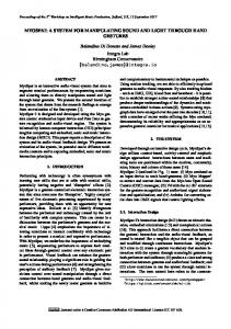
To implement the fast marching method, we needed to solve three key problems: (i) formulation of the speed function, (ii) initialization of the seed points and (iii) determination of the stopping criterion. We formulate the speed function based on the gradient magnitude. The speed function is defined as an exponential function of the gradient magnitude; that is, F = exp(γ||∇I||), where γ is a negative constant and I is the original image. Although the curvature of the contours can also be combined into the speed function, we found that this usually did not enhance the results of all our experiments on the tomographic data we used. Initialization of the seed points are essential for correct segmentation of the components of interest. There are several ways to choose the initial seed points: mechanically by a user, using “balloons”, or by the locus of the zero-crossing of the Laplacian of the smoothed images (see [61] for a summary). Our previous work on gradient vector diffusion [79, 80] provides an efficient way to automatically locate relevant contour seed points. The gradient vector field derived from the original images (or volumes) is diffused and the critical points are used as our seeds. All seed points are grouped into two classes: feature seeds and background seeds. For example, if the features to be segmented have higher intensities than the background, then the feature seeds are the maximum critical points where all the neighboring gradient vectors point toward those voxels while the background seeds are the minimum critical points where all the neighboring gradient vectors point away from those voxels. Additional sub-groups may be chosen for applications requiring multi-material segmentation. The stopping criterion of the marching contours is another important issue in the fast marching method. The fast marching algorithm described in [48] does not give an explicit stopping criterion such that the more expensive level set method had to be used to finalize the segmentation. In addition, like the fast marching method, even the level set method may have to deal with the “leaking” problem around the boundary gaps. In our current implementation for tomographic imaging data, we address this problem using dual contours: one starting from the feature seeds and the other starting from the background seeds. In the beginning, a contour is initialized at each seed point. Since all the seeds are classified into two (or more) groups, all the initial contours are accordingly classified into these groups. Each of the contours march (grow) simultaneously according to Eq.(3). Whenever two contours from the same group meet, they merge into a single contour. On the other hand, if two contours from different groups meet, both contours stop marching on the common boundaries. Both situations are illustrated in Fig.1, where we can see that the dual contours stop automatically. With an appropriate parameter γ in the speed function F , we can guarantee that dual contours from different groups stop correctly on their common boundaries where the magnitude of the image gradient is locally maximal. An interesting observation is that the seed points obtained in our method are quite similar to the seeds used in the watershed immersion method [69], and the marching process in our method is analogous to the immersion process. However, our method considers the image gradient, an important feature of image boundaries, which is not taken into account in the watershed immersion method. In addition, our method allow merging between similar group contours, starting from different seeds, which avoids the oversegmentation problem as commonly seen in the watershed immersion method.
9
(a) Initial contours
(b) Marching contours
(c) Merged contours
Figure 1: Fast marching method using dual-contours. (a) We only consider four seed points in this image. The two blue contours correspond to the maximum critical points while the other two contours (red) correspond to the minimum critical points. (b) Wheneve dual contours with different colors meet, they prevent each other from moving.(c) When dual contours with the same color meet, they merge into a single contour, and keep growing.
3.4
Skeleton Extraction
Extracting iso-surfaces is very sensitive to the selection of iso-values. In addition, tracing isosurfaces followed by boundary-based skeleton extraction is computationally intensive. In this section we compute the skeletons directly from gray-scale volumes without extracting iso-surfaces. To construct the critical Morse complex, we begin from critical points and trace integral linking curves by traversing the gradient vector field in their principal (”eigen”) directions. The constructed Morse complex, however, is not exactly what we want in many applications. The Morse complex is a “skeleton” of the entire volume but we are more interested in the “skeleton” of the features that we want to extract. Therefore, we need to prune the Morse complex, retaining only those critical points and their associated integral curves that correspond to the features of interest. For example, if the intensities of features are brighter than those of the background, we should ignore the minimum critical points and only consider the maximum and saddle critical points and the integral linking curves between them. Given a 3D gray-scale volume, how can we correctly locate the appropriate critical points? If the volume is ideally smooth, the critical points can be easily computed from the first and second derivatives of the volume. However, noisy data may cause too many critical points detected and thus result in a superfluous and incorrect Morse complex. Anisotropic filtering is excellent for noise reduction while preserving sharp edges. However, this method may not be the best way to compute the critical points because an anisotropic filter may result in “flat” regions near the centers of the features such that the gradient vectors in that region vanish. Therefore, the “flat” regions make it difficult to exactly locate the critical points. An interesting thing is that in this particular case, Gaussian or other isotropic filters perform better than anisotropic filtering. But as we mentioned above, Gaussian filtering tends to smooth small features that are close to “stronger” features. In order to improve the robustness of small feature during noise reduction, we instead use the gradient vector diffusion approach [75, 79, 80], which differs from classical 10
Figure 2: Computing critical points using gradient vector diffusion. A gray-scale 2D image is shown on the right, where a sub-region is considered for computing the gradient vector field. The vector diffusion algorithm discussed in [79] is applied and shown on the left. Five critical points are located including two maximal critical points (green), two minimal critical points (purple) and one saddle critical point (yellow). The diffused gradient vector field is also used to tracing the integral linking curves in order to construct the Morse graph. filters in that it smoothes the gradient vectors, not the gray-scale intensities. An advantage of this method is that we can control the smoothing based on the directions of the vectors. The smoothed (or diffused) gradient vector field is used to locate the critical points. Critical points corresponding to local maxima are those points where all the surrounding vectors point to these points. Similarly, critical points corresponding to local minima are those points where all the surrounding vectors point away from these points. Critical points corresponding to saddles are detected at those points where some surrounding vectors point to these points from both sides along some directions while the other surrounding vectors point away from these points from both sides along the other directions. Fig.2 demonstrates a two-dimensional example, where all these three types of critical points are detected using gradient vector diffusion.
4
Interactive Volume Exploration Tool
The volume-rendering client can act as a 3D roving microscope, allowing users to visualize data that is too large to fit on a single machine. The graphical user interface allows for interactive visual selection of transfer function and isocontour, aka the contour spectrum [8, 56]. The user interface also allows the user to move and resize the sub-volume window. The data within the sub-window is then transmitted by the server to the client computer, and displayed interactively using fast texture based volume rendering that can be combined with rendered geometry [72, 58]. The rover connects to a data server that contains large datasets. The server can extract and resample sub-volumes of different sizes, which are then transmitted to the client for visualization.
11
Figure 3: Overview of Volume Rover and selection of sub-region of interest via Volume Rover. The full resolution dataset (with a size of 1024 × 1024 × 100 voxels) shown on the right comprises two adjacent bullfrog hair bundle stereocilia connected by a tip link. The selected sub-volume shown on the left has a much smaller size (about 120 × 240 × 50 voxels), which makes feature interpretation as well as visualization much faster and easier.
12
The client downloads data differentially, by only downloading the data that the client does not already have cached. The Rover contains two views. One view contains a volume render of a sub-sampled version of the entire volume. The user specifies the sub-volume by interacting with a cuboid located in the sub-sampled volume. At the center of the cuboid are 3 axes, one for each dimension. The user can translate the sub-volume by clicking on one of these axes and then dragging along the axis. At the end of each axis is a resizing knob. The user can resize the sub-volume window by clicking on one of the resizing knobs and dragging along its corresponding axis. The user can also rotate the sub-window around each of its axes. After the user manipulates the sub-volume window, the client requests a sub-volume of the correct size and resolution from the data server. The data is downloaded from the server and rendered using fast texture-based volume rendering. The data for the rover can either come from a remote data server , or can come from the local hard disk. In either case, if the data requested is too large to fit into graphics memory, it is filtered using Gaussian filtering and sub-sampled. The sub-sampled data is then loaded into the video card and rendered using texture based volume rendering. The Rover can visualize volumes up to 512x256x256 imaging without resampling. When data come from the hard disk, the rover automatically caches a pyramid hierarchy of sub-sampled volumes. For each volume, the Rover filters and resamples the volume, creating a volume with half the resolution of the original volume. This process is repeated until the lowest resolution volume is 1x1x1. This speeds up the interactive exploration of the data since the data does not have to be resampled for every extraction. In addition to the volume rendering, the user can request to see an isosurface rendering of the data. The rover performs isosurface extraction on the sub-volume portion of the data as well as the thumbnail data. The surface is rendered together with the volume. If the user moves the sub-volume, the rover obtains the new data and performs the isosurface extraction again. The new surface and new sub-volume are then rendered together. This allows the user to interactively explore the volume render as well as the isosurface render of the large data. During the volume exploration or feature extraction process, it is also necessary on ocassion to zoom in to crop out volumetric regions of interest. The selected sub-region is then used for faster noise reduction and selected feature segmentation. The direct manipulation GUI (graphical user interface) of the Volume Rover allows us to visually identify an select specific volumetric sub-regions of interest (as shown in Fig.3). Furthermore, the user can request a bilateral filtering, an anisotropic geometric diffusion evolution, a gradient vector diffusion, and skeleton feature extraction on the data set. The rover will then perform the filtering and feature extraction on the extracted sub-volume. If an isosurface is being rendered, it will be re-extracted from the newly filtered data. The new data is then displayed together with the new isosurface.
13
Figure 4: Bilateral pre-filtering coupled with an anisotropic diffusion filter. Shown on the left is a sub-volume of the original dataset comprising extracellular links between a stereocilium and the kinociliar bulb in a bullfrog macular sensory epithelia hair bundle. The picture on the right shows the filtered result within the same region as the one on the left.
5
Applications and Results
All the techniques discussed in previous section were tested on real electron tomograms. We first demonstrate the performance of our anisotropic diffusion filter coupled with bilateral prefiltering. Fig.4 shows the difference between the original volume and the filtered one. The anisotropic diffusion filter clearly reduces the noise level while enhancing the features. In Fig.5 and Fig.6, we show two examples of our segmentation method on filtered and contrast-enhanced volumes. The one in Fig.5 segments the kinociliar links of a hair bundle. For better result, the segmentation is restricted to the extracellular region. This can be easily done by classifying all the critical points outside that region into one group such that all the contours starting from those critical points will be merged. Fig.6 shows the segmented tip link between bullfrog hair cell stereocilia. It is worth noting that the criterion for classifying critical points may differ from data to data. All the maximum (or minimum) critical points may not necessarily classified into one group. Quite often we need to classify the maximum critical points with intensities below a threshold into the group of minimum critical points. Similarly some minimum critical points with intensities above a threshold (could be different from previous one) may be classified into the group of maximum critical points. As we said before, sometimes more than two groups may be necessary. In Fig.5 and Fig.6, we consider only two groups, corresponding to feature and background respectively. Fig.7 gives an example of skeleton extraction. The skeletons are extracted by simplifying the Morse graph of the density map. We first filter the original data and then the contrast enhancement is applied. The gradient vector field is then computed and diffused using the vector 14
Figure 5: Boundary segmentation on sub-volume of bullfrog hair bundle kinociliar links. The original volume is first filtered and then the contrast is enhanced before we apply boundary segmentation. The left picture shows a slice with the segmented boundaries indicated by red curves. The picture in the middle gives a 3D volume-rendered view of the segmented boundaries. Shown on the right is a closer look at the segmented boundaries.
Figure 6: Boundary segmentation on a sub-volume of the bullfrog hair bundle tip link. The original volume is first filtered and then contrast enhanced before boundary segmentation. The left picture shows a slice with the segmented boundaries indicated by red curves. The middle and right pictures give 3D volume-rendered views from two different directions.
15
Figure 7: Simplified Morse graph on a sub-volume of the bullfrog hair cell actin bundle. The original volume is first filtered and then contrast enhanced before we extract and simplify the Morse graph. Left: volume-rendering of the filtered and contrast-enhanced density map. Middle: simplified Morse graph extracted from the same region, where the actin bundles and the links between them are clearly shown. Right: simplified Morse graph embedded in the density map. diffusion technique (Eq.(2)). The critical points are then located from the gradient vector field (see Fig.2). However, only those critical points corresponding to features are recognized and all other critical points are considered invalid. The Morse graph is constructed by tracing the integral linking curves along the diffused gradient vector field. Since we only consider a subset of the critical points, the obtained Morse graph is just a simplified version of the original Morse graph but it is more faithful to the true skeletons of the features under investigation.
6
Conclusion
We have presented algorithms for fully automatic volume filtering, boundary segmentation and skeletonization, and have successfully applied it to cell and molecular tomographic imaging data. We have also developed an interactive volumetric exploration tool (Volume Rover) which encapsulates implementations of the above filtering, and curve/surface feature extraction algorithms, and additionally uses multi-resolution interactive geometry and volume rendering, for the visualization. This interactive visualization tool runs under both Linux and Win2K desktop platforms, and is available for free download under the GNU public license, from http://www.ices.utexas.edu/CCV/software.html.
Acknowledgments This research is supported in part by NIH grant DC00241, NSF grants ACI-9982297, CCR9988357, and from grant UCSD 1018140 as part of NSF-NPACI, Interactive Environments 16
Thrust. Thanks are also due to Anthony Thane for development of the Volume Rover Tool, to Qiu Wu for his implementation of the bilateral and anisotropic diffusion filtering, and to Dr. Ulrike Ziese and Bram Koster at University of Utrecht for recording the tomographic tilt series. Manfred Auer would also like to thank Dr. Da Neng Wang (Skirball Institute, NYU), his mentor Dr. Jim Hudspeth as well as the Human Frontier Science Program Organization, and the Jane Coffin Childs Memorial Fund for Medical Research / Agouron Institute for postdoctoral fellowships.
References [1] B. Alberts. The cell as a collection overview of protein machines: Preparing the next generation of molecular biologists. CELL, 92:291–294, 1998. [2] C. Arcelli and G.S. Baja. Euclidean skeleton via centre-of-maximal-disc extraction. Image and Vision Computing, 11(3):163–173, 1993. [3] M. Auer. Electron cryo-microscopy as a powerful tool in molecular medicine. J. Molecular Medicine, 78:191–202, 2000. [4] C. Bajaj, I. Ihm, and S. Park. Visualization-specific compression of large volume data. In Proc. of Pacific Graphics, pages 212–222, Tokyo, Japan, 2001. [5] C. Bajaj, V. Pascucci, and D. Schikore. Visualization of scalar topology for structural enhancement. In IEEE Visualization, pages 51–58, 1998. [6] Chandrajit Bajaj, Insung Ihm, and Sanghun Park. 3D RGB image compression for interactive applications. ACM Transactions on Graphics, 20(1):10–38, 2001. [7] Chandrajit Bajaj and Brian Mirtich. Level-set based volumetric anisotropic diffusion for 3d image denoising. In ICES Technical Report, University of Texas at Austin, 2002. [8] Chandrajit Bajaj, Valerio Pascucci, and Dan Schikore. The Contour Spectrum. Proceedings of IEEE Visualization ’97, pages 167–175, November 1997. [9] Chandrajit Bajaj, Valerio Pascucci, and Daniel R. Schikore. Fast isocontouring for improved interactivity. In Proceedings of the 1996 Symposium for Volume Visualization, pages 39–46, 1996. [10] Chandrajit Bajaj and Daniel R. Schikore. Error-bounded reduction of triangle meshes with multivariate data. In Proceedings of Visual Data Exporation and Analysis III, SPIE vol 2656, pages 34–45, 1996. [11] D. Barash. A fundamental relationship between bilateral filtering, adaptive smoothing and the nonlinear diffusion equation. IEEE Trans. on Pattern Analysis and Machine Intelligence, 24(6):844–847, 2002. 17
[12] W. Baumeister and A. C. Stevens. Macromolecular electron microscopy in the era of structural genomics. TIBS, 25:624–631, 2000. [13] J. Bohm, Frangakis, R. Hegerl, S. Nickell, D. Typke, and W. Baumeister. Toward detecting and identifying macromolecules in a cellular context: template matching applied to electron tomograms. Proc Natl Acad Sci., 97:14245–14250, 2000. [14] V. Caselles, J.L. Lisani, J.M. Morel, and G. Sapiro. Shape preserving local histogram modification. IEEE Trans. Image Processing, 8(2):220–230, 1998. [15] R. Deriche. Fast algorithm for low-level vision. IEEE Trans. on Pattern Recognition and Machine Intelligence, 12(1):78–87, 1990. [16] K. Dierksen, D. Typke, R. Hegerl, A.J. Koster, and W. Baumeister. Towards automatic electron tomography. Ultramicroscopy, 40:71–87, 1992. [17] D.L. Donoho and I.M. Johnson. Ideal spatial adaptation via wavelet shrinkage. Biometrika, 81:425–455, 1994. [18] F. Durand and J. Dorsey. Fast bilateral filtering for the display of high-dynamic-range images. In ACM Conference on Computer Graphics (SIGGRAPH), pages 257–266, 2002. [19] H. Edelsbrunner, J.Harer, and A.Zomorodian. Hierarchical morse complexes for piecewise linear 2-manifolds. In ACM Symposium on Computational Geometry, pages 70–79, 2001. [20] H. Edelsbrunner, D. Letscher, and A. Zomorodian. Topological persistence and simplification. Discrete and Computational Geometry, 28(4):511–533, 2002. [21] M. Elad. On the bilateral filter and ways to improve it. IEEE Transactions On Image Processing, 11(10):1141–1151, 2002. [22] R. J. Ellis. Macromolecular crowding: obvious but underappreciated. Trends Biochem. Sci., 26(10):597–604, 2001. [23] W.Baumeister et. al. Electron tomography of molecules and cells. Trends Cell Biol., 9:81– 85, 1999. [24] A. Frangakis and R. Hegerl. Noise reduction in electron tomographic reconstructions using nonlinear anisotropic diffusion. J. Struct. Biol., 135, pages =, 2001. [25] Achilleas S. Frangakis and Reiner Hegerl. Segmentation of two- and three-dimensional data from electron microscopy using eigenvector analysis. Journal of Structural Biology, 138(1-2):105–113, 2002. [26] J. Frank. Electron Tomography. Plenum Press, 1992. [27] R. Glaeser. Electron crystallography: present excitement, a nod to the past, anticipating the future. J. Struct. Biol., 128:3–14, 1999. 18
[28] R.C. Gonzalez and R.E. Woods. Digital image processing. Addison-Wesley, 1992. [29] T. Grogorishin, G. Abdel-Hamid, and Y.H. Yang. Skeletonization: An electrostatic fieldbased approach. Pattern Analysis and Application, 1(3):163–177, 1996. [30] A. Ben Hamza and Hamid Krim. Image denoising: A nonlinear robust statistical approach. IEEE Transactions on Signal Processing, 49(12):3045–3054, 2001. [31] A. Ben Hamza, P. Luque, J. Martinez, and R. Roman. Removing noise and preserving details with relaxed median filters. Journal of Mathematical Imaging and Vision, 11(2):161– 177, 1999. [32] M.L. Harlow, D. Ress, A. Stoschek, R.M. Marshall, and U.J. McMahan. The architecture of active zone material at the frog’s neuromuscular junction. Nature, 409:479 – 484, 2001. [33] J.C. Hart. Morse Theory for Implicit Surface Modeling. [34] R. Hart. Electron microscopy of unstained biological material: The polytropic montage. Science, 159:1464–1467, 1968. [35] David Hessler, Stephen J. Young, and Mark H. Ellisman. A flexible environment for the visualization of three-dimensional biological structures. Journal of Structural Biology, 116(1):113–119, 1996. [36] W. Hoppe, J. Gassmann, N. Hunsmann, H.J. Schramm, and M. Sturm. Three-dimensional reconstruction of individual negatively stained yeast fatty-acid synthetase molecules from tilt series in the electron microscope. Hoppe-Seyler’s Z. Physiol. Chem., 355:1483–1487, 1974. [37] D.J. Jobson, Z. Rahman, and G.A. Woodell. A multiscale retinex for bridging the gap between color images and the human observation of scenes. IEEE Trans. Image Processing, 6(7):965–976, 1997. [38] D.J. Jobson, Z. Rahman, and G.A. Woodell. Properties and performance of a center/surround retinex. IEEE Trans. Image Processing, 6(3):451–462, 1997. [39] T.A. Jones, J-Y. Zou, S.W. Cowan, and M. Kjeldgaard. Improved methods for building protein models in electron density maps and the location of errors in these models. Acta Crystallogr., 409:110–119, 1991. [40] R. Kimmel, D. Shaked, N. Kiryati, and A.M. Bruckstein. Skeletonization via distance maps and level sets. Computer Vision and Image Understanding, 62(3):382–391, 1995. [41] A.J. Koster, H. Chen, J.W. Sedat, and D.A. Agard. Automated microscopy for electron tomography. Ultramicroscopy, 46:207–227, 1992.
19
[42] J.R. Kremer, D.N. Mastronarde, and J.R. McIntosh. Computer visualization of threedimensional image data using imod. J Struct Biol, 116:71–76, 1996. [43] A.F. Laine, S. Schuler, J. Fan, and W. Huda. Mammographic feature enhancement by multiscale analysis. IEEE Trans. Medical Imaging, 13(4):725–738, 1994. [44] L. Lam, S.W. Lee, and C.Y. Suen. Thinning methodologies - a compresensive survey. IEEE Trans. on Pattern Analysis and Machine Intelligence, 14(9):869–885, 1992. [45] Yanhong Li, Ardean Leith, and Joachim Frank. Tinkerbell-a tool for interactive segmentation of 3d data. Journal of Structural Bioloby, 120(3):266–275, 1997. [46] J. Lu, D.M. Healy, and J.B. Weaver. Contrast enhancement of medical images using multiscale edge representation. Optical Engineering, 33(7):2151–2161, 1994. [47] G. Malandain and S.F. Vidal. Euclidean skeletons. Image and Vision Computing, 16(5):317– 327, 1998. [48] R. Malladi and J.A. Sethian. A real-time algorithm for medical shape recovery. In IEEE International Conference on Computer Vision, pages 304–310, 1998. [49] M. Marko and A. Leith. Sterecon - three-dimensional reconstructions from stereoscopic contouring. Journal of Structural Biology, 116(1):93–98, 1996. [50] B.F. McEwen, K.H. Downing, and R.M. Glaeser. The relevance of dose-fractionation in tomography of radiation-sensitive specimens. Ultramicroscopy, 60:357–373, 1995. [51] B.F. McEwen and J. Frank. Electron tomographic and other approaches for imaging molecular machines. Curr. Op. Neurobiol., 11:594–600, 2001. [52] B.F. McEwen and M. Marko. Three-dimensional electron micros-copy and its application to mitosis research. Methods Cell Biol, 61:81–111, 1999. [53] B.F. McEwen and M. Marko. The emergence of electron tomography as an important tool for investigating cellular ultrastructure. J. Histochem Cytochem, 49:553–563, 2001. [54] R.L. Ogniewicz and O. Kubler. 28(3):343–359, 1995.
Hierarchic voronoi skeletons.
Pattern Recognition,
[55] P. Perona and J. Malik. Scale-space and edge detection using anisotropic diffusion. IEEE Trans. on Pattern Analysis and Machine Intelligence, 12(7):629–639, 1990. [56] Hanspeter Pfister, Bill Lorensen, Chandrajit Bajaj, Gordon Kindlmann, Will Schroeder, Lisa Sobierajski Avila, Ken Martin, Raghu Machiraju, and Jinho Lee. The transfer function bake-off. IEEE Transactions on Computer Graphics and Applications, 21(3):16–22, 2001. [57] W.K. Pratt. Digital Image Processing (2nd Ed.). A Wiley-Interscience Publication, 1991. 20
[58] S. R¨ottger, M. Kraus, and T. Ertl. Hardware-accelerated volume and isosurface rendering based on cell-projection. In Proceedings of IEEE Visualization ’00, pages 109–116, 2000. [59] J.A. Sethian. A marching level set method for monotonically advancing fronts. Proc. Natl. Acad. Sci., 93(4):1591–1595, 1996. [60] J.A. Sethian. Level Set Methods and Fast Marching Methods, 2nd edition. Cambridge University pPress, 1999. [61] J. Shah. A common framework for curve evolution, segmentation and anisotropic diffusion. In International Conference on Computer Vision and Pattern Recognition, pages 136–142, 1996. [62] Bong-Soo Sohn, Chandrajit Bajaj, and Vinay Siddavanahalli. Feature based volumetric video compression for interactive playback. In Preceedings of the IEEE/ACM Siggraph 2002 Symposium for Volume Visualization and Graphics, pages 89–96, 2002. [63] J.A. Stark. Adaptive contrast enhancement using generalization of histogram equalization. IEEE Trans. Image Processing, 9(5):889–906, 2000. [64] Arne Stoschek and Reiner Hegerl. Denoising of electron tomographic reconstructions using multiscale transformation. Journal of Structural Bioloby, 120(3):257–265, 1997. [65] K.A. Taylor, H. Schmitz, M.C. Reedy, Y.E. Goldman, C. Franzini-Armstrong, H. Sasaki, R.T. Tregear, K. Poole, C. Lucaveche, R.J. Edwards, L.F. Chen, H. Winkler, and M.K. Reedy. Tomographic 3d reconstruction of quick-frozen, ca2+-activated contracting insect flight muscle. Cell, 99:421–431, 1999. [66] C. Tomasi and R. Manduchi. Bilateral filtering for gray and color images. In 1998 IEEE International Conference on Computer Vision, pages 836–846, 1998. [67] M. van Heel, B. Gowen, R. Matadeen, EV. Orlova, R. Finn, T. Pape, D. Cohen, H. Stark, R. Schmidt, M. Schatz, and A. Patwardhan. Single-particle electron cryo-microscopy: towards atomic resolution. Q Rev Biophys, 33:307–369, 2000. [68] Marc van Kreveld, Rene van Oostrum, Chandrajit Bajaj, Valerio Pascucci, and Daniel Schikore. Contour trees and small seed sets for isosurface traversal. In Symposium on Computational Geometry, pages 212–220, 1997. [69] Niels Volkmann. A novel three-dimensional variant of the watershed transform for segmentation of electron density maps. Journal of Structural Biology, 138(1-2):123–129, 2002. [70] Niels Volkmann and Dorit Hanein. Quantitative fitting of atomic models into observed densities derived by electron microscopy. Journal of Structural Biology, 125(2-3):176–184, 1999.
21
[71] J. Weickert. Anisotropic Diffusion In Image Processing. ECMI Series, Teubner, Stuttgart, ISBN 3-519-02606-6, 1998. [72] R. Westermann and E. Thomas. Efficiently using graphics hardware in volume rendering applications. In In SIGGRAPH ’98, pages 169–177, 1998. [73] W. Wriggers and S. Birmanns. Using situs for flexible and rigid-body fitting of multiresolution single-molecule data. J. Struct. Biol., 133:193–202, 2001. [74] Willy Wriggers, Ronald A. Milligan, and J. Andrew McCammon. Situs: A package for docking crystal structures into low-resolution maps from electron microscopy. Journal of Structural Biology, 125(2-3):185–195, 1999. [75] C. Xu and J.L. Prince. Snakes, shapes, and gradient vector flow. IEEE Trans. Image Processing, 7(3):359–369, 1998. [76] Y. Xu, J. B. Weaver, D. M. Healy, and J. Lu. Wavelet transform domain filters: A spatially selective noise filtration technique. IEEE Trans. Image Processing, 3(6):747–758, 1994. [77] I.T. Young and L.J. Vliet. Recursive implementation of the gaussian filter. Signal Processing, 44:139–151, 1995. [78] Z. Yu and C. Bajaj. Anisotropic vector diffusion in image smoothing. In Proceedings of International Conference on Image Processing, pages 828–831, 2002. [79] Z. Yu and C. Bajaj. Image segmentation using gradient vector diffusion and region merging. In Proceedings of International Conference on Pattern Recognition, pages 941–944, 2002. [80] Z. Yu and C. Bajaj. Normalized gradient vector diffusion and image segmentation. In Proceedings of European Conference on Computer Vision, pages 517–530, 2002.
22