Vortex Dynamics SIMulation Hans Fangohr University of Southampton United Kingdom
[email protected] August 25, 2007
$Header: /Users/svn/cvs/VD/V1/docu/usage.tex,v 1.19 2006/10/09 03:51:38 fangohr Exp $ $Name:
1
$
2
CONTENTS
Contents 1 Introduction 1.1 What is this document about? . . . . . 1.2 Who could be interested in this? . . . . 1.3 So what can this software do? . . . . . . 1.4 What is the future of this project? . . . 1.5 What is the structure of this document?
. . . . .
. . . . .
. . . . .
. . . . .
. . . . .
. . . . .
. . . . .
. . . . .
. . . . .
. . . . .
. . . . .
. . . . .
. . . . .
. . . . .
. . . . .
. . . . .
. . . . .
. . . . .
. . . . .
. . . . .
. . . . .
. . . . .
. . . . .
3 3 3 3 4 4
2 Quick tour
4
3 Preparing a run 3.1 The configuration file . . . . . 3.2 The parameter file . . . . . . 3.3 The creation of the parameter 3.4 Output from vdsimpp . . . .
. . . .
5 5 5 5 6
4 Running the simulation 4.1 Watch progress of simulation while computing . . . . . . . . . . . . . . . . . . . . 4.1.1 Display in real computation time . . . . . . . . . . . . . . . . . . . . . . . 4.1.2 Analyse data while computing . . . . . . . . . . . . . . . . . . . . . . . .
8 8 8 8
. . . . file . .
. . . . . . . . . . . . . . (vdsimpp) . . . . . . .
. . . .
. . . .
. . . .
. . . .
. . . .
. . . .
. . . .
. . . .
. . . .
. . . .
. . . .
. . . .
. . . .
. . . .
. . . .
. . . .
. . . .
. . . .
. . . .
5 Post-processing of data 5.1 How much data is stored? . . . . . . . . 5.2 Processing a range of time steps . . . . 5.2.1 Select range . . . . . . . . . . . . 5.2.2 Skip every nth time step . . . . . 5.2.3 Looking at individual time steps 5.3 Extract observables . . . . . . . . . . . . 5.3.1 Overview . . . . . . . . . . . . . 5.4 Histogram of positions . . . . . . . . . . 5.5 Vortex configuration at one time step . 5.5.1 Delaunay triangulation . . . . . . 5.5.2 Topological defects . . . . . . . . 5.5.3 Vortex positions . . . . . . . . . 5.6 Track down one vortex . . . . . . . . . . 5.7 Time-dependant observables . . . . . . . 5.7.1 Centre of mass . . . . . . . . . . 5.7.2 Topological defects . . . . . . . . 5.7.3 Local hexatic order . . . . . . . . 5.8 The other vdpp: vdpp2 . . . . . . . . . . 5.9 Histogram of vortex velocities . . . . . . 5.10 What else . . . . . . . . . . . . . . . . .
. . . . . . . . . . . . . . . . . . . .
. . . . . . . . . . . . . . . . . . . .
. . . . . . . . . . . . . . . . . . . .
. . . . . . . . . . . . . . . . . . . .
. . . . . . . . . . . . . . . . . . . .
. . . . . . . . . . . . . . . . . . . .
. . . . . . . . . . . . . . . . . . . .
. . . . . . . . . . . . . . . . . . . .
. . . . . . . . . . . . . . . . . . . .
. . . . . . . . . . . . . . . . . . . .
. . . . . . . . . . . . . . . . . . . .
. . . . . . . . . . . . . . . . . . . .
. . . . . . . . . . . . . . . . . . . .
. . . . . . . . . . . . . . . . . . . .
. . . . . . . . . . . . . . . . . . . .
. . . . . . . . . . . . . . . . . . . .
. . . . . . . . . . . . . . . . . . . .
. . . . . . . . . . . . . . . . . . . .
. . . . . . . . . . . . . . . . . . . .
. . . . . . . . . . . . . . . . . . . .
. . . . . . . . . . . . . . . . . . . .
. . . . . . . . . . . . . . . . . . . .
. . . . . . . . . . . . . . . . . . . .
9 9 9 9 10 10 10 10 10 11 11 13 13 15 15 15 16 17 17 17 18
6 Case-study: current-voltage curve 6.1 Introduction . . . . . . . . . . . . . . 6.2 Configuration file . . . . . . . . . . . 6.3 Creation of pinning potential . . . . 6.4 Anneal vortices into pinning surface 6.5 Apply increasing driving force . . . . 6.6 End of simulation . . . . . . . . . . .
. . . . . .
. . . . . .
. . . . . .
. . . . . .
. . . . . .
. . . . . .
. . . . . .
. . . . . .
. . . . . .
. . . . . .
. . . . . .
. . . . . .
. . . . . .
. . . . . .
. . . . . .
. . . . . .
. . . . . .
. . . . . .
. . . . . .
. . . . . .
. . . . . .
. . . . . .
. . . . . .
19 19 19 19 20 20 21
. . . . . .
. . . . . .
3
1 INTRODUCTION 7 Advanced creation of pinning surfaces 7.1 How is pinning data stored for vdsim . . . . . . . . 7.2 The vdconvert tool . . . . . . . . . . . . . . . . . 7.2.1 Converting pinning potential files formats . 7.2.2 How to export/import pinning data to other s/tools? . . . . . . . . . . . . . . . . . . . . 7.3 Superimposing different pinning structures . . . . . 8 Loose collection of remarks 8.1 Continue run or restart from scratch 8.2 Simulation methods . . . . . . . . . 8.3 Dimensionality . . . . . . . . . . . . 8.4 Simulation units . . . . . . . . . . . 8.5 Verbosity . . . . . . . . . . . . . . . 8.6 Man pages . . . . . . . . . . . . . . .
. . . . . .
. . . . . .
. . . . . .
. . . . . .
. . . . . .
. . . . . .
. . . . . .
. . . . . .
. . . . . . . . . . . . . . . . . . . . . . . . . . . . . . . . . . . . . . . . . . . . . . . . . . . (not supported) application. . . . . . . . . . . . . . . . . . . . . . . . . . . . . . . . . . . . . . . .
. . . . . .
. . . . . .
. . . . . .
. . . . . .
. . . . . .
. . . . . .
. . . . . .
. . . . . .
. . . . . .
. . . . . .
. . . . . .
. . . . . .
. . . . . .
. . . . . .
. . . . . .
. . . . . .
22 22 22 22 22 23 24 24 25 25 25 25 26
References
26
A Configuration file
27
B Parameter file
30
C Mini introduction to xmgrace
32
D Man pages D.1 Overview D.2 vdsimpp . D.3 vd.par . . D.4 vdpp . . . D.5 vdpp2 . .
33 33 35 37 40 45
. . . . .
. . . . .
. . . . .
. . . . .
. . . . .
. . . . .
. . . . .
. . . . .
. . . . .
. . . . .
. . . . .
. . . . .
. . . . .
. . . . .
E To do
1 1.1
. . . . .
. . . . .
. . . . .
. . . . .
. . . . .
. . . . .
. . . . .
. . . . .
. . . . .
. . . . .
. . . . .
. . . . .
. . . . .
. . . . .
. . . . .
. . . . .
. . . . .
. . . . .
. . . . .
. . . . .
. . . . .
. . . . .
. . . . .
. . . . .
. . . . .
. . . . .
46
Introduction What is this document about?
This text provides an introduction into the Vortex Dynamics simulation software which is developed mainly by Hans Fangohr at the University of Southampton.
1.2
Who could be interested in this?
If you want to model the vortex state numerically, then this software could be able to do the job, and save you lots of time implementing it yourself.
1.3
So what can this software do?
At the moment, the software fully supports overdamped Langevin Dynamics in two-dimensions with a variety of vortex-vortex interaction potentials, complete freedom to choose a (spatially homogenous) time-dependant Lorentz fore and any desired pinning potential, with periodic and open boundary conditions. By the time this is written, the simulation is capable to do much more, including MonteCarlo simulations, 3d-vortex state simulations (using a substrate model, or using several coupled
2 QUICK TOUR
4
layers), the use of a new “passive” pinning, and Hybrid-Monte-Carlo runs. However, those are partly not fully tested, and not documented (yet). Therefore, for the time being users are advised to stick to the 2d-Langevin case, which provides sufficiently rich physics to be able to spend years investigating it. There are a number of publications using this software (for example [1, 2, 3, 5, 4, 6]).
1.4
What is the future of this project?
It is hoped that Hans will be able to continue working on the software, to • finish documentation of existing features • finish implementation and testing of partly implemented/tested features • implement new features as required by him, or other users. If you want to get involved1 in this, then contact
[email protected]. Similarly, if you spot anything which looks like a bug, or you don’t understand this document, or the manpages, or the program’s behaviour, then please get in contact. Finally, if you want to suggest an extension, then this is welcome as well.
1.5
What is the structure of this document?
Section 2 provides a very brief overview of how to run simulations. The subsequent sections 3 to 8 detail how to prepare, run, and analyse a simulation. It is recommended to read this section to get a feel for the possibilities the software provides. Eventually, section 8 contains a collection of remarks which might be worth knowing at some point. (It is hoped that they will be presented in a more structered way one day).
Now go ahead, and have fun!
2
Quick tour
Here is the ultra-condensed description of a typical computation: • Edit configuration file (for example runID=sample, so the file is sample.cnf) to describe the (experimental) situation one wants to simulate • Create parameter file sample.par by exectuting “vdsimpp sample” • Run the simulation by executing “vdsim sample” • postprocess output with the help of vdpp and vdpp2 • and use xmgrace, vdconvert and openDX (or other standard packages of your choice) to study (the post-processed) output. The next sections will give more details on each of those points. 1
The software is written in C++, and compiles on Linux systems (and possibly on Unix as well).
5
3 PREPARING A RUN configuration file (.cnf) edited by user contains meta data Example: contains magnetic field, intended number of vortices, shape of simulation cell (aspect ratio)
parameter file (.par) created by vdsimpp contains final parameters as will be used by vdsim Example: contains the actual number of vortices used, and the size (in x- and y-direction) of the simulation cell
Table 1: Comparison of configuration and parameter file.
3 3.1
Preparing a run The configuration file
Each run has one configuration file (.cnf) which inucludes all parameters of the run, and the name of the run — the run-ID. The configuration file must be called runID.cnf. We start with the sample.cnf configuration you find in the sample subdirectory. Look into the file using a simple text editor (such as xemacs, emacs, pico, joe, vi,. . . ). You will find in the beginning of each line a keyword, followed by a value. For example: runID
sample
#how many vortices nVortices 400 #which ratio of the x and y-length of the system do you want LxLyRatio 1
So the runID is “sample”. Lines starting with “#” are comments and ignored by the software. The requested number of vortices is 400. The file is much longer, and please go ahead and study it. The comments in the file should explain most of the keywords. The complete configuration file for this example is shown in A.
3.2
The parameter file
We have to create a parameter file from the configuration file. This file spells out (nearly) all parameters as used in the simulation. The simulation programm (with name vdsim) will read its parameters from this file. See table 1 to see how the parameter file compares with the configuration file.
3.3
The creation of the parameter file (vdsimpp)
The parameter file is created by calling the Vortex Dynamics SIMulation Parameter Prepration program (vdsimpp). The program vdsimpp takes a runID as a parameter, then attempts to open and read the file runID.cnf. The runID can contain a path (i.e. myruns/runID.cnf). vdsimpp then parses the configuration file, and creates a parameter file (runID.par) if all necessary information has been found in the configuration file runID.cnf. There will are a couple of plausibility checks which are performed, and either a warning is issued (to stdout, which is usually the screen), or if fatal problems are detected, an error is reported (to both stdout and stderr) and the program is aborted. Read the manpage for vdsimpp for more details (see section 8.6. In our example, we would do vdsimpp sample and the program will reply with
6
3 PREPARING A RUN main(): ################################################################ # Vortex Dynamics Simulation (vdsimpp) # # ../vdsimpp sample # # Last modification $Date: 2006/10/09 03:51:38 $ # Release $Name: $ # Revision $Revision: 1.19 $ # Author $Author: fangohr $ # # Sat Mar 9 14:16:17 2002 ################################################################ Metaconf::compute_parameters(): Changed n from 400 to 418 (2*19*11)
The last line tells us, that while we requested 400 vortices, for the given value for the magnetic induction and the required x-y-ratio of the simulation cell (as both specified in sample.cnf), the program has chosen 418 vortices. The reason for this is that 418 vortices fit in the simulation cell in the form of a hexagonal lattice. In other words, this choice avoids frustratration. To be more precise, vortices are arranged in 19 times 11 unit cells, each containing two vortices (those are the numbers in parathesis), to form a hexagonal lattice. The created parameter file starts with the following lines: Configuration: { runID nVortices simulation_type nLayers Lengthx Lengthy LxLyRatio start_timestep stop_timestep rand_seed dt eta mass
sample 418 MDLangevin 1 16.1815600380339 16.22632239197948 0.9972413740548066 0 2000 -1 0.005 1 0
From this we see that we have 418 vortices, the length of the simulation cell is ≈ 16.18 in x and ≈ 16.22 in y-direction, and thus the aspect ratio is 0.9972413740548066, which is fairly close to the value 1.0 we requested in sample.cnf. The complete parameter file for this example is shown in B.
3.4
Output from vdsimpp
In addition to the parameter file as shown above, vdsimpp creates a couple of other files: If support for Grace (see www.plasmagate.weizmann.ac.il) has been compiled into vdsimpp, then vdsimpp creates the following grace project files: runID_actions_temp.agr runID_actions_lor_x.agr runID_actions_lor_y.agr runID_actions_pin_str.agr
Temperature Lorentz force (x-component) Lorentz force (y-component) Pinning strength
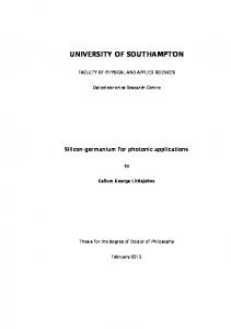
It also creates corresponding postscript files of those plots (ending .ps instead of .agr). For the sample-configuration described here, the tempererature changes at different timesteps as specified in the configuration file:
7
3 PREPARING A RUN Action events for changing temperature, runID=sample 10
10
10
temperature
8
6
4 3 2
2 1
00 0
3
2
1
0
0
500
0
1000
0
1500
0
2000
time steps Sat Mar 9 15:06:11 2002
Figure 1: Graphical representation of the temperature as a function of time(steps). This plot is created by vdsimpp and can be seen using, for example, by typing “ghostview runID actions temp.agr” in a shell.
Action Action Action Action Action Action Action
0 temp 0 100 temp 300 temp 500 temp 700 temp 1300 temp 1800 temp
1 2 3 0 10 0
and this can be seen in runID_actions_temp.agr. To see the file use xmgrace runID_actions_temp.agr , or use ghostview to see the post-script version ghostview runID_actions_temp.agr”. The output is shown in figure 1. If a smooth cut-off [1, 2] is used, then vdsimpp creates runID_c_forceplot.agr and runID_c_energyplot.agr, and the corresponding postscript files. The _c_ stands for Control, as those plots can be used to verify that the smooth cut-off does what the user expects. In particular for small systems the smoothed interaction energy may have a minimum at a distance smaller than the cut-off distance. This is a problem resulting from choosing too small a system (or cut-off if given explicitly). vdsimpp attempts to detect such minima in the smoothed interaction and issues an error if a minimum is spotted. However, it is always useful to be able to verify that things are working as expected. If the run (as specified in runID.cnf) requires data for a pinning potential, then the pinning potential is read by vdsimpp. This ensures that the files are in the right place. It also detects corrupted pinning data files. If the run (as specified in runID.cnf) requires data for a meissner potential, then the meissner potential is read by vdsimpp. We have now the relevant files in place to start the computation.
8
4 RUNNING THE SIMULATION
4
Running the simulation
The simulation is started with the command vdsim runID, so in our example it would be vdsim sample. The program vdsim reads sample.par, and starts the computation as specified in that file. First, a the configuration is printed to the screen, and then estimates of the required time to complete the run are printed: TIME: Sat Mar 9 15:30:59 2002( 0.6%)ET:00:16:15Sat Mar TIME: Sat Mar 9 15:31:05 2002( 1.2%)ET:00:16:15Sat Mar TIME: Sat Mar 9 15:31:11 2002( 1.7%)ET:00:17:12Sat Mar TIME: Sat Mar 9 15:31:17 2002( 2.3%)ET:00:17:44Sat Mar Simulation::do_actions(void): time step 100: set temperature TIME: Sat Mar 9 15:31:23 2002( 2.8%)ET:00:17:44Sat Mar TIME: Sat Mar 9 15:31:29 2002( 3.4%)ET:00:17:28Sat Mar TIME: Sat Mar 9 15:31:35 2002( 4.1%)ET:00:17:04Sat Mar
9 15:47:08 2002 9 15:47:08 2002 9 15:48:05 2002 9 15:48:37 2002 to 1.000000 9 15:48:37 2002 9 15:48:21 2002 9 15:47:57 2002
Each “TIME”-line states first the current time, then the amount of the computation done which is 0.% in the first line above. This is followed by the Estimated Time (ET) that the simulation needs in total to finish (here around 16 to 17 minutes), followed by the date and time at which the completion of the run is expected. The estimate may vary as the system load of your computer can vary, particularly in multi-user environments. The timing estimate is printed approximately every 5 seconds in the first 3 minutes of a run, every 5 minutes thereafter, and only every 30 minutes after the first half an hour of computation. Other statements are printed occasionally, so for example the message that the temperature has been set to 1 at time step 100 (as was required in the parameter file). The example shown above was computed on a 200MHz Pentium I, so it is very likely to be much faster an any other machine one can find nowadays . . . .
4.1 4.1.1
Watch progress of simulation while computing Display in real computation time
It is possible to watch the progression of the simulation as it computes using a special data file. The line that has to be uncommented (or added, if missing) in the configuration file is datafile grace special. Every time step data is saved to disk (i.e. every save interval steps), the new positions are sent to a running instance of xmgrace. Note that if save interval is small (and your computer is not too fast) lots of cpu-time can be used up by the frequent transfer of data to grace, and its efforts to display it. In other words, if you experience a remarkable slow down in the response of your system to mouse-clicks, then consider increasing the value of save interval. This option is only suitable if the program is running on a workstation with X. It is useful to play with parameters to quickly see howe the system reacts. Once a good parameter set has been found, the computation should be done without this feature. Not using the real-time display to saves (CPU) time, and allows to run the code on cluster of work stations (without needing X). Eventually, note that if you (accidentally) close the xmgrace-window, the simulation will start complaining, and lots of cpu-time is being used by printing those error messages. Thus, for production purposes this feature should not be used. 4.1.2
Analyse data while computing
It is also possible to analyse the data-files while a computation is running (using vdpp as described in section 5). This is the recommended way of investigating the process of a simulation. (We don’t expect vdpp2 to work reliable when the calculation is still ongoing.)
5 POST-PROCESSING OF DATA
5
9
Post-processing of data
The program vdpp is used to Post-Process Vortex dynamics Data.2 The program vdpp2 is another program to post-process vortex dynamics data, and has been written later (2006). It using the vdpp program to extract the raw data from the data files and then carries out additional analysis in the programming language Python. The only reason for having two programs (vdpp and vdpp2) that do complimentary tasks, is that it is more efficient to do many post processing tasks in a high level language. Consequently, it is much easier to extend the functionality of vdpp2 should any new features be required.
5.1
How much data is stored?
To learn about the data we have now on disk, use vdpp sample (that is assuming that your runID is “sample”). The program answers with: setup_range(): Have 81 timesteps, starting at 0 and ending at 2000 main(): No options have been chosen that produce output. Leaving program now.
Remember that using the -v-switch more detailled information can be obtained (see section 8.5), so if we run vdpp sample -v3, we get Data::read_ttab(): Read 81 timesteps, starting at 0 and ending at 2000 main(): processing parameter ’-v3’ setup_range(): Have 81 timesteps, starting at 0 and ending at 2000 setup_range(): 0 25 50 75 100 125 150 175 200 225 250 275 300 325 350 375 400 425 450 475 500 525 550 575 600 625 650 675 700 725 750 775 800 825 850 875 900 925 950 975 1000 1025 1050 1075 1100 1125 1150 1175 1200 1225 ... 2000 main(): No options have been chosen that produce output. Leaving program now.
This tells us in more detail which time-steps are available.
5.2 5.2.1
Processing a range of time steps Select range
To process only a subset of the stored time steps, we use the range switch. For example, to look only at time-steps 500 to 1000, we say vdpp sample -range 500 1000 -v3 : setup_range(): Have 21 timesteps, starting at 500 and ending at 1000 main(): No options have been chosen that produce output. Leaving program now.
Again, using -v3, we can see explicitly which time steps there are in the range of 500 to 1000: ... setup_range(): Have 21 timesteps, starting at 500 and ending at 1000 setup_range(): 500 525 550 575 600 625 650 675 700 725 750 775 800 825 850 875 900 925 950 975 1000 ... 2
Admittedly, the choice of names for the PreParation of a SIMulation (vdsimpp) and the for the Post-Processing (vdpp) is not the best one.
5 POST-PROCESSING OF DATA 5.2.2
10
Skip every nth time step
To skip every 2nd time step, we modify the above command to be vdpp sample -range 500 1000 2 -v3 : (note the 2 after 1000 and before -v3) ... setup_range(): Have 11 timesteps, starting at 500 and ending at 1000 setup_range(): 500 550 600 650 700 750 800 850 900 950 1000 ...
5.2.3
Looking at individual time steps
To investigate time step 500, we can use the Time Step-switch -ts in the following manner: vdpp sample -ts 500. There are two special cases for the first and the last time step: it is legal to use -ts first and -ts last. This is particularly useful to look at the last time step of a running simulation if one doesn’t know which number it is. As always, more details can be found in the man-page, and by calling the programm incorrectly: try vdpp sample -range to get help on -range, and vdpp sample -ts to get help on -ts.
5.3 5.3.1
Extract observables Overview
There is a variety of switches for vdpp to extract information from the data files. All switches can be combined with the range-switches as explained in section 5.2. An overview is of possible options is given in table 2. The man-page (see section 8.6) contains a detailed description of all the options. In the next sections, we show a couple of examples how to look at the data.
5.4
Histogram of positions
Assume we want to study the melting transition of a vortex system without pinning. Our example sample.cnf starts with vortices in hexagonal positions and increases the temperature from timesteps 100 to 1000. This is the right idea to study melting, but clearly in a proper simulation there should be many more intermediate temperatures, and much more timesteps at each temperature. However, for the demonstration of the availabe features this will do nicely. To look at the distribution of vortex positions between time steps 100 and 1000, we create a 2d-histogram of the positions. We choose a resolution of 200 times 200 pixels, and issue the command: vdpp sample -range 100 1000 -hist 200 200 This creates a file sample_pp_poshist0.bin, which contains the histogram in a binary data format. The file name is composed of the runID, the extension pp, which stands for PostProcessed data, the word hist to indicate that it is a histogram, and the number 0, because it is the histogram for layer 0. This will be helpful for multi-layer runs (not fully implemented yet). The data format is the same as the binary format chosen by Gnuplot. We provide a program vdconvert that can convert such binary data in a variety of formats. For example, we can convert3 the histogram data into a png-file via: vdconvert sample pp poshist0.bin test.png 3
This requires the Magick++ suite to be installed.
11
5 POST-PROCESSING OF DATA -dump [pos] [vel] [for] [act] -hist NX NY -range START [STOP [STEP]] -ts TS | first | last -dummy -cm -disp [0|mean] -BG [STARTTIMESTEP] -ft KX KY [KX KY ] [..] -cift N [rad][phi0][range] -svp [NL NP]...[NL NP] -snap3d [ZSCALE [SPLPTS]] -snapgrace -def [L] -delsnap2d [L] -delsnap3d -hop [L] -anghist NBIN [L] -diffpos [cm] -avgvel -ivp -Alex1 -pov -sbao
(dump data to stdout) Create histogram of positions with NX times NY grid cells define range of time steps to process define one time step (TS) to process run in only-pretending-to-do-something mode compute centre of mass position, velocity, meansqr displ. compute displacement of pancakes compute B(x) =< [u(0) − u(x)]2 > compute Fourier transform (FT) √ for k = 2π/a0 (KX, KY ) compute FT for |k| = 4π/a0 / 3∗rad at N k’s ouput Single Vortex Positions (Layer NL, particle NP) create snapshots of single timesteps (for Geomview) create snapshots of single timesteps (for Grace) compute nr of topological defects compute 2d delaunay triangulations (for Geomview) compute 3d delaunay triangulation (for Geomview) computes the Hexagonal Order Parameter computes a histogram of bonding angles with NBIN bins computes displacement between 1. and last step (2d only) computes vortices’ indiv. time-avged velocity (2d,MG) store plain positions in file (use for restarting) variety of options to analyse substrate potiential produce output for povray (as on title page) Simon Bending Array Occupany
Table 2: Overview of options for vdpp. This list can be obtained by calling vdpp without further parameters. The precise meaning of each option is described in the vdpp-man page.
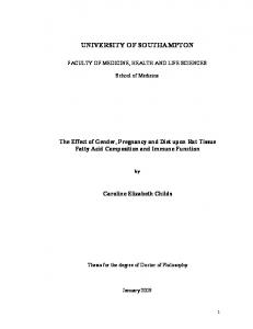
and look at the file using xv test.png. The output, reflecting a hexagonal lattice (because the temperature was lower than the melting temperature, and there were not enough time steps to allow melting anyway) is shown in figure 2. We can also create data for OpenDX using vdconvert sample pp poshist0.bin test.dx . Figure 3 shows the plot created with OpenDX. Alternatively, the data in sample pp poshist0.bin can be read into Matlab using readgnu.m as provided in tools/matlab. Another option to plot those data (altough maybe less suited for higher resolutions) is gnuplot. The command in gnuplot is splot "sample pp poshist0.bin" binary with lines, and the reprensentation looks nice with contour-lines, i.e. set contour base; replot. Note that in the computation of this histogram only the time steps stored in the data files have been used. There is another option to create a histogram which consideres all time steps. If you want to use this, have a look at the “shist’’ commands which are explained in sample.cnf.
5.5 5.5.1
Vortex configuration at one time step Delaunay triangulation
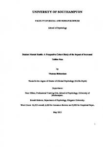
To see the vortex configuration at, say time step 500, we do vdpp sample -ts 500 -snapgrace This creates a file sample_pp_snapgrace_del500.agr, which we can plot using xmgrace sample pp snapgrace del500.agr The name indicates the runID (sample), post-processed data (pp), it’s a SNAP shot for GRACE, and it includes a Delaunay triangulation (del). All that for time step 500. The output is shown in figure 4. Another file with name sample pp snapgrace.agr is created as well. It has the same content
5 POST-PROCESSING OF DATA
12
Figure 2: Histogram of vortex positions for sample-run between time steps 100 and 1000. Resolution is 200x200 pixels. (Note: we have inverted the colours, i.e. black becoms white, in order to save toner for printed versions).
Figure 3: Same data as in figure 2 but visualized using OpenDX. Note that the spikyness of the data is not suprising since we have only averaged 37 time steps.
13
5 POST-PROCESSING OF DATA
sample sample_pp_snapgrace_del500.agr 8 7 6 5 4 3 2 1 0 -1 -2 -3 -4 -5 -6 -7 -8 -8
-7
-6
-5
-4
-3
-2
-1
0
1
2
3
4
5
6
7
8
Figure 4: Snap shot of vortex positions at time step 500. The Delaunay triangulation shows that there are no topological defects.
as xmgrace sample pp snapgrace del500.agr, but a more convienient name so it is easier to type xmgrace sample pp snapgrace.agr. Note that this file will be overwritten if we use vdpp ...-snapgrace the next time. 5.5.2
Topological defects
In time step 1300 in sample.cnf we have set the temperature to a high value of 10. This is above the melting temperature, and therefore topological defects develop. We can use the same switch -snapgrace to see those. Figure 5 shows the output. The positions of the defects are stored in plain ascii text in sample pp snapgrace def1500.dat. This can be used for further analysis. 5.5.3
Vortex positions
To extract vortex positions at one time step as pure data (to be used in another plotting programme, the -ivp option can be used: vdpp sample -ts 500 -ivp creates a file sample pp ivp 500.dat which can be plotted, for example in gnuplot (via plot "sample pp ivp 500.dat"), or xmgrace (via xmgrace plot "sample pp ivp 500.dat", or any other 2d-plotting application (Excel, . . . ).
14
5 POST-PROCESSING OF DATA
sample sample_pp_snapgrace_del1500.agr 8 7 6 5 4 3 2 1 0 -1 -2 -3 -4 -5 -6 -7 -8 -8
-7
-6
-5
-4
-3
-2
-1
0
1
2
3
4
5
6
7
8
Figure 5: Snap shot of vortex positions at time step 1500. Topological defects with 7 neareast neighbours are highlighted by blue circels, and defects with 5 nearest neighbours by red circles.
15
5 POST-PROCESSING OF DATA
Vortex 0 sample_pp_svp_0_000.txt
-6.6 -6.8
x-pos y-pos
-7 -7.2 -7.4 -7.6 -7.8 -8 0
500
1000
time steps
1500
2000
Figure 6: x and y-components of position r = (x, y) of vortex 0. Note how the actions (as defined in the configuration and parameter file) are reflected in the motion of the vortex: at time step 100 thermal fluctuations set in, with increasing magnitude up to time step 700, where the temperature is reduced to 0 again. Then the system relax which is reflected in the smooth damped motion of the vortex until time step 1000. Then, a Lorentz force in x-direction, and 100 time steps later in y-direction acts, which results in a motion with constant velocity. At time step 1300 a very high temperature is applied with results in a break down of the hexagonal lattice and a relatively pronounced change of position of the vortex. Temperature is set back to zero at time step 1800, after which the system relaxes. In time step 1999 the vortices are (artificially) set back to their initial positions, which is clearly visible.
5.6
Track down one vortex
To follow the path of one vortex, we use the Single Vortex Position-switch -svp: vdpp sample -svp 0 0 The two zeros indicate that we want to get the path of particle in layer 0 (that is the first zero), and in that layer we want particle number 0. The data is written to sample pp svp 0 000.txt and a graphical representation is created using xmgrace -nxy sample pp svp 0 000.txt and shown in figure 6.
5.7 5.7.1
Time-dependant observables Centre of mass
Even though the vortices are assumed to be massless, we can compute the centre of mass of the system by averaging the vortex positions. The command is vdpp sample -cm and this creates files • sample pp cmpos.txt containing the position centre of mass
16
5 POST-PROCESSING OF DATA
centre of mass velocity
x-component y-component
1
0.5
0 0
500
1000
time steps
1500
2000
Figure 7: x and y-components of the centre of mass velocity of the vortex system. Note how the actions (as defined in the configuration and parameter file) are reflected in the motion of the centre of mass of the system: at time step 100 thermal fluctuations set in up to time step 700, where the temperature is reduced to 0 again. If the system was infinitely large, we would not expect the centre of mass to move under thermal fluctuations. However, since we have a finite system, the centre of mass performs a random walk. At time step 1000 , a Lorentz force in x-direction, and 100 time steps later in y-direction acts, which results in a motion with constant velocity, until the force is set to zero. At time step 1300 a very high temperature is applied which again results in slight changes of the centre of mass, and thus the velocity of it. In time step 1999 the vortices are (artificially) set back to their initial positions, which results in a huge (negative) velocity of the centre of mass..
• sample pp cmvel.txt containing the velocity of the centre of mass • sample pp mnsd.txt containing the MeaN Square Displacement !
The mean-square displacement ∆r 2 (t) = N1 i (ri (t0 ) − ri (t))2 is a measure for the average distance vortices have moved away from their positions at the first time step at time t0 . It can be used as a measure for diffusion: in a solid this quantity will be constant (assuming vortices stay in their lattice positions) whereas for a liquid it increases with time. The data in all those files contain the time step in the first coloumn, the x-component of the quantity in the second and the y-component in the third coloumn. The data, for example the center of mass velocity, can be plotted using xmgrace -nxy sample pp cmvel.txt which is shown in figure 7. 5.7.2
Topological defects
The number of topological defects is computed using vdpp sample -def and the result can be plotted via xmgrace sample pp def.txt.
17
5 POST-PROCESSING OF DATA
1
local hexatic order
0.8
0.6
0.4
0.2
0
500
1000
time steps
1500
2000
Figure 8: Shown is the local hexatic order of the system, which is 1.0 for a hexagonal lattic (the starting configuration). As soon as thermal fluctutainos set in at time step 100, it reduces with increasing temperature. At time step 700, temperature is set to 0, and the system relaxes back into a hexagonal lattice. This relaxation continues even when the Lorentz force starts acting at time step 1000. Only when an even higher temperature than before is applied at time step 1300, the hexatic order decreases again. This time, the lattice brakes down, and the order parameter drops under 0.5. At time step 1800 the temperature is zero again, and the system tries to minimise its energy which increases the hexatic order. Since in time step 1999 the vortices are (artificially) set back to their initial positions, the local hexatic order parameter jumps discontinuosly back to 1.0.
5.7.3
Local hexatic order
We compute local Hexagonal Order Parameter (hop) as described in [1, 2] This parameter is 1.0 for a perfect hexagonal lattice, and goes towards zero for a liquid. It is computed using the -hop-switch. The data is written to sample pp hop.txt, and can be plotted using xmgrace sample pp hop.txt. The plot is shown in figure 8.
5.8
The other vdpp: vdpp2
Currently, vdpp2 supports only very few functions. Use vdpp --help to get an overview of these features.
5.9
Histogram of vortex velocities
One of the analysis capabilities of vdpp2 is to compute the time averaged velocity histogram of the vortex system. We give an example: vdpp2 --average-velocity --stopts 1800 sample This will compute the average velocity of all vortices from time step 0 (default) to timestep 1800 (as specified with the --stopts switch) of the “sample” run. It takes into account that the periodic boundary conditionts may move a vortex back to the ’other side’ of the simulation cell and adds the length of the simulation cell to correct this (should such a ’wrapping’ event occur).
18
5 POST-PROCESSING OF DATA
25
number of vortices
20
15
10
5
0
0.1
0.12 0.14 0.18 0.2 0.16 average velocity of vortex (time steps 0 to 1800)
0.22
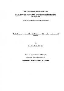
Figure 9: The average vortex velocity for the ’sample’ run. The average has been taken from time step 0 to time step 1800. The plot has been created with xmgrace. The spread of the velocities comes from the thermal fluctuations. The overall move of ≈ 0.015 comes from the applied lorentz forces. The spread of the velocities here comes from the thermal fluctuations.
Then, this total displacement is divided by the simulation time that has passed (this is the number of time steps from start time step to stop time step multiplied with dt (as in the .par file) in simulation units). Finally, the obtained averaged velocities are written into a file RUNID_pp_avg_vel_tsX-Y.txt where X is the start time step and Y the the stop time step (where here RUNID is “sample”, X is 0, and Y is 1800). The first column contains the x componenent of the averaged velocity, the second column the y component, the third coloumn the magnitude. Each row corresponds to one vortex. A second set of three files with names RUNID_pp_avg_vel_tsX-Y_histogram_Z.txt is written where Z can be ’v’, ’vx’ and ’vy’. Each of those files contains histogram data for the corresponding average velocities. The default is 50 bins (but can be modified with the –histogram-bins switch). To plot the histogram, we can for example use this command: xmgrace sample_pp_avg_vel_ts0-1800_histogram_v.txt The resulting plot (with the colors of the bars changed, and some labelling of the axes added) is shown in figure 9.
5.10
What else
There is more out there, including the computation of structure factors (Fourier transforms), histograms of bond-angles of the Delaunay triangulations, production of output for povray to produce nicely rendered animations, and more. Do go ahead and study the man page for vdpp. If there are any questions, please report them to
[email protected].
6 CASE-STUDY: CURRENT-VOLTAGE CURVE
6
19
Case-study: current-voltage curve
6.1
Introduction
Assume we want to study the current voltage curve of a system of vortices in a random pinning potential. In principle we will 1. create a pinning potential 2. put vortices into pinning potential (maybe using annealing?) 3. apply a very small driving force (so that vortices don’t start moving yet) 4. increase this driving force every n-thousand time steps (and vortices will start moving) 5. stop increasing the driving force and stop simulation at some point.
6.2
Configuration file
You can use the provided file iv.cnf as a sample to start from (in directory V1/examples/iv). The important bit in iv.cnf is that we include pinning #do we want pinning pinning true #if yes, a pinning file can be specified pinfile iv_pin0.bin
# default name is IN_pin0.bin (for 2d-runs)
#strength of pinning (choose negativ values for passive pinning) pin_str 2 # pinning_interpolation bicubic # or bilinear (default)
and that we specify a pinning strength (here 2). The
6.3
Creation of pinning potential
To be able to create a pinning potential, we need the file iv.par which we get by running vdsimpp iv. You should get a warning that no pinning file has been found (but that’s okay because we have not created any yet). Now that we have iv.par, we can create a pinning potential. The required program is vdpin. Type just ‘‘vdpin’’ to get an overview of features of vdpin. To create a pinning surface from scratch, the -n (for New) switch is the best choice. (If you have pinning potential stored as gray-values in a bitmap, you could use -a to Add a lengthscale to it and to be able to use it in the simulation.) Try to type ‘‘vdpin -n’’ to get an overview of possible new pinning potentials. The output could look like this: ewpinning(): -nrg -nrs -npd -nsb
Possible values for -n are runID npins width depth NX NY seed for Random Gaussian runID sitedist (in L) pointspersite seed for Random Splines runID sitedistx sitedisty width depth g_dist for Periodic Dots runID scale g_dist Simon Bending’s sample, periodic magnet dots
Let’s distribute a set of Gaussian point-like pins. Therefore, we will use -nrg. Assume that we want 100 pins, each of width 0.1 (in units of lambda). The depth does not really matter as the whole pinning will be re-scaled so that the mean-square force is 1.0 f0 (set depth to 1 in example below). The values NX and NY determine the resolution of the pinning matrix (i.e. the number of pixels to represent the pinning and we choose 300 and 300). Eventually, the seed determines the starting point for the random number generator, which determines the positions
6 CASE-STUDY: CURRENT-VOLTAGE CURVE
20
of the pins (we choose 2, any integer will do). Note that the depth of the pins is constant in our example (not normally distributed as in some papers) and the position of the pins is random. So, a possible call to vdpin would be: vdpin -nrg iv 100 0.1 1 300 300 2 and the result is shown in figure 10.
Figure 10: Point-like pinning. Left: gray-scale plot. Right: 3d-presentation using Geomview (convert the iv pin0.bin like this ”vdconvert iv pin0.bin output.mesh and then visualise it with geomview output.mesh) Note that the left upper corner of the grayscale (on the left) has been rotated to the front left corner in the right-hand plot. Alternatively, to get a smoothly varying pinning potential (more like intrinsic pinning), you can use the -nrs option. The site-distance is the distance of the coarse lattice points which are assigned random heights (uniform distribution of heights) and between which we interpolated “pointspersite”-points using cubic splines (in order to get a smooth potential). Here is an example with coarse points every 0.15 λ, and 4 intermediate points between each coarse point (random seed=2): vdpin -nrs iv 0.15 3 2 The resulting pinning potential is shown in figure 11.
6.4
Anneal vortices into pinning surface
One can anneal the vortices into the pinning potential to find a starting configuration that is well pinned. To do this, the temperature in the simulation has to be reduced slowly from a value above the melting temperature to zero. The time-steps 100 to 7500 in iv.cnf demonstrate this schematically. If a stable configuration is important, then different annealing speeds and initial temperatures should be tested. (Note that the melting temperature depends on the time-step and the pinning. See seperate documentation for this.) In other words, in the beginning of the run, we anneal the vortices into the pinning potential.
6.5
Apply increasing driving force
In time-step 10,000 to 210,000 we increase the driving force every 3000 steps. Again, don’t take this as good practise, it is only meant to demonstrate the system. Many more timesteps at each
6 CASE-STUDY: CURRENT-VOLTAGE CURVE
21
Figure 11: Smoothly varying pinning. Left: gray-scale plot. Right: 3d-presentation using Geomview showing only a part of the complete simulation cell (convert the iv pin0.bin like this ”vdconvert iv pin0.bin output.mesh -crop 0 2 0 2 and then visualise it with geomview output.mesh. This will create the plot on the right handside which shows the area [0..2] × [0..2] of the simulation cell.)
driving force should be run to ensure the system has enough time to find a steady state at that drive.
6.6
End of simulation
After having finished the simulation, the usual techniques to extract and visualise data can be used. See section 5 for a reminder on post-processing data. Probably, the most important data for current-voltage studies is the centre of mass position and the centre of mass velocity of the system. They can be obtained using vdpp iv -cm. This will create files iv pp cmpos.txt and iv pp cmvel.txt. The first contains data like this: 0 50 100 150 200 250 300 350 400 450
0.0341826 0.0361866 0.0335337 0.0320023 0.0307934 0.0346323 0.0284829 0.0270439 0.0264438 0.0232934
-0.182811 -0.187288 -0.185291 -0.191717 -0.187844 -0.189425 -0.190254 -0.190613 -0.187431 -0.188012
where the first column is time step, the second column is the x-component of the centre of mass and the third column is the y-component of the centre of mass. The data in this file can be plotted in the standard way (using xmgrace, gnuplot or whatever one likes).
7 ADVANCED CREATION OF PINNING SURFACES
7
22
Advanced creation of pinning surfaces
7.1
How is pinning data stored for vdsim
It is worth knowing roughly how the simulation stores pinning potential. Any pinning potential that may use, is a function f (x, y) of the two independent spacial coordinates x and y. Often, we can specify this function analytically (for example a superposition of Gaussian curves each representing one columnar pin). However, this is not always possible, and even if we can specify the equation, it may be computational expensive to evaluate that expression again and again (for every vortex in every time step). The approach chose here is that we sample f (x, y) at discrete points (xi , yj ) with i ∈ 0, 1, 2, . . . , Nx and j ∈ 0, 1, 2, . . . , Ny and store this discretised version of f (x, y) in a matrix. For values between of f between the grid points, some interpolation is used (there are at least two interpolation options). This means that we need to create a file that stores this matrix. The ’intrinsic’ file format of vdsim are matrix file4 with the extension bin. (This format is very similar to GNUPLOTs binary format.) These keep the data in binary (always in Little Endian independent of hardware) and can be read quickly. For each of these files, there is a second file with extension bin.comment that carries some additional data. This format can be converted into a number of formats using vdconvert. The approach of storing the data in a file and interpolating between grid points also allows to use arbitrary pinning potentials. For example, if an experimental method would provide a grayscale plot of the the true pinning potential, then this could be converted into a bitmap file (and then into a .bin-file using vdconvert) and be used as a pinning potential in the simulation. (Technical note: for Molecular Dynamics (and Langevin Dynamics) runs, we need the force that results from this pinning potential. This is evaluated numerically from the potential matrix.)
7.2
The vdconvert tool
The vdconvert program is essential when creating more complicated pinning potentials. 7.2.1
Converting pinning potential files formats
The vdconvert tool that comes with the software allows to convert the simulations own data format for pinning data into other formats, including bitmaps. This is done very similar to the convert command that comes with ImageMagick by just specifying the required filename with extension. We could, for example, convert the pinning file from the iv case study (section 6) into a bitmap with this command:5 vdconvert iv pin0.bin test.png The file test.png will contain a bitmap in png format that can be displayed with xview, ImageMagick or other tools. The grayscale corresponds to height of the pinning potential. As usual, the vdconvert command provides a brief guide to its capabilities when called without parameters. 7.2.2
How to export/import pinning data to other (not supported) applications/tools?
Other useful conversion examples include: vdconvert iv pin0.bin test.txt This will create a text file containing all the values of the potential in the following format: The first two integer numbers NX and NY indicate how many coloumns and rows there are. The 4 Note that the ’matrix’ file also contains information about the positions xi and yj for which the columns and rows of the matrix hold the values of f (xi , yj ). 5 Note that the conversion into bitmaps is only possible if ImageMagick support has been compiled into the executables.
7 ADVANCED CREATION OF PINNING SURFACES
23
next NX numbers are the x-positions of the grid points. The next line starts with the y-position of the first grid row followed by NX numbers with the data for this row. The next line starts with the y-position of the second grid row followed by NX numbers with the data for that row. In total, there are NY rows with data. The very last line of the file can contain a comment which is optional. This text file presentation can be used to convert the pinning data into any required format to visualise it. Note that it is also possible to convert such a text-pinning data file back to the normal binary representation: vdconvert test.txt iv pin0.bin This allows to compute a required pinning potential in any other language or tool. Once this is done, it can be written in the txt format as described, and converted into a binary pinning file.
7.3
Superimposing different pinning structures
Suppose you would like to study the effect of a few strong pins together with less correlated random pinning. We use the earlier example iv example to demonstrate this. Starting from the iv.cnf file as provided with the distribution, we need to create the iv.par file with vdsimpp iv Subsequently, we can create several pinning potential using the vdpin command and add them together (we can also scale their relative magnitudes). Because our aim here is to combine two different pinning potentials, we need to work a bit harder and rename some files in the process. Here is a complete example: First we create the random pinning potential (as in figure 11, see text section 6.3): vdpin -nrs iv 0.15 3 2 This command has created the iv pin0.bin file that contains the pinning potential. We now need to save this file under another name (we also copy the .comment file although this is not strictly necessary): mv iv pin0.bin iv pin0 uncorrelatedpins.bin mv iv pin0.bin.comment iv pin0 uncorrelatedpins.bin.comment At this stage, we should find out how many pixels are used in this pinning potential so that we can generate the next potential (which will be superimposed to this one) with the same resolution (i.e. number of pixels in x and y direction). To find out the number of pixels we use these bash commands which will store the number of pixels in variables Nx and Ny. vdconvert iv_pin0_uncorrelatedpins.bin tmp.stat cat tmp.stat | grep Nx cat tmp.stat | grep Ny Nx=‘cat tmp.stat | grep Nx | head -n 1 | awk ’{print $3}’‘ Ny=‘cat tmp.stat | grep Ny | head -n 1 | awk ’{print $3}’‘ (We could also just look at the tmp.stat file in a text editor (and would find that Nx=343 and Ny=328.) Now we create the second pinning potential with strong pins with same number of pixels: vdpin -nrg iv 20 0.3 0.3 N xNy 1 (or just type vdpin -nrg iv 20 0.3 0.3 343 328 1 This has created the new iv pin0.bin file with the strong pins (compare with figure 10) and the explanations in section 6.3. Now we save this file somewhere: mv iv_pin0.bin iv_pin0_strongpins.bin mv iv_pin0.bin.comment iv_pin0_strongpins.bin.comment
8 LOOSE COLLECTION OF REMARKS
24
Figure 12: The mixed pinning potential. Now the exciting bit starts: we can build a linear combination of the two potentials. To demonstrate this, assume we want to make the strong pins half as strong as their default value: vdconvert iv pin0 strongpins.bin iv pin0 strongpinsscaled.bin -mult 0.5 And finally, we add the pinning potentials together: vdconvert iv pin0 strongpinsscaled.bin iv pin0 final.bin -add iv pin0 uncorrelatedpins.bin The resulting potential is shown in figure 12. (We created the figure with this comand: vdconvert iv pin0 final.bin myfigure.eps .) Note that we need to choose the right name for the final file for the simulation to load it (check iv.par if in doubt which name is required): mv iv_pin0_final.bin iv_pin0.bin mv iv_pin0_final.bin.comment iv_pin0.bin.comment Now we could run the simulation as usual: vdsim iv and do some postprocessing as usual: vdpp iv -cm
8 8.1
Loose collection of remarks Continue run or restart from scratch
Suppose you have started a simulation via vdsim sample, and then it is interrupted (say the process is killed due to CTRL+C being pressed, or the scheduler stopped the job on a cluster). Then the computation can be continued from the last stored time step by just starting it again, i.e. vdsim sample. If, on the other hand, the configuration file has been changed, and the parameter file updated (through vdsimpp), then you want to start again from the start-time step, and not from the last time step stored in the previous run. In this case the command vdclear runID will delete all data files, and the subsequently started simulation vdsim runID will start again from the start time step.
25
8 LOOSE COLLECTION OF REMARKS
8.2
Simulation methods
The code is in principle able to use • Langevin dynamics • Monte Carlo methods • Molecular Dynamics • Hybrid method in order to study the physics of the vortex state. Molecular Dynamics (behaviour of particles is like atoms in vacuum: they have inertial mass, and there is no friction) is only useful a tool for Hybrid method runs. The Hybrid method is still under develope ment. The Monte-Carlo method has been used to verify the Langevin method (for example for melting of a clean system one gets the same melting temperature with both methods), but does no yet support all the featurs (missing or at least not tested is using a Meissner field for example.) The conservative choice which should allow to study most experimental conditions is Langevin Dynamics. The sample configuration files in this document use Langevin Dynamics.
8.3
Dimensionality
The simulation is fully working for two-dimensional systems. The code is prepared to be able to compute layered systems, but this is not fully implemented and tested. It is advised to stick to the 2d case, as long as you don’t want to continue programming the 3d-case.
8.4
Simulation units
All numbers in the simulation are expressed in dimensionless simulation units. What are those numbers? The short answer is to look into the parameter file, where there is the following section: Scaling_parameters:{ scale.T scale.Gamma scale.L scale.t scale.f0 }
6.003760454554897 K 0.0025 (recipr=400) 1.4e-07 m 1.466851242491835e-10 2.368312519085602e-13
s Nm (f0*a0=0.176247616285282eV)
This has to be read as follows. A length x in the simulation, corresponds to a length xL in SI-units, where L =scale.L=1.4e-07m. Similarly, T is the scaling parameter for temperature, t for time, f0 for forces. The more detailed explanation (including analytical expressions) is currently in preparation.
8.5
Verbosity
All programs of the vortex dynamics simulation suite understand the switch -v?, where ? is a number ranging from 0 to 5. With this verbosity switch the amount of progress and diagnostic messages can be determined. The meaning of the numbers is as follows: 0 silent – no output messages 1 progress only – minimal output
REFERENCES
26
2 warnings (default) – issue more information, and warnings 3 more warnings – be more picky than 2 4 debug – lots of information 5 extreme debug – extremely detailed information The default value 2 (warnings) is a sensible choice. However, if something goes wrong (i.e. an error occurs), it might be worth re-running the program with a higher verbosity value; possibly the additional messages provide a clue what went wrong.
8.6
Man pages
There is a couple of man-pages in preparation, and partly finished. The files are in the mansubdiretory. Each file starts with the name of the program it describes, and is followed by .1, such as vdpp.1. The files are written in the standard unix man-page style, and could be studied using the man command if they were in the man-search path. If this is not possible, one can type groff -Tascii -man vdpp.1 | less to see the file nicely displayed. Alternatively, use the showmanfile-command, which just includes this sequence, i.e. type “showmanfile vdpp.1”. There are also postscript and ascii-versions of the man-pages in the ps and txt subdirectories. We have further included some of these page in the appendix D.
References [1] H. Fangohr, A. R. Price, S. J. Cox, P. A. J. de Groot, G. J. Daniell and K. S Efficient methods for handling long-range forces in particle-particle simulations. Journal of Computational Physics, 162, 372–384 (2000). [2] H. Fangohr, S. J. Cox and P. A. J. de Groot. Vortex dynamics in two-dimensional systems at high driving forces. Physical Review B, 64, 064505 (2001). [3] H. Fangohr, P. A. J. de Groot and S. J. Cox. Critical transverse forces in weakly pinned driven vortex systems. Physical Review B, 63, 064501 (2001). [4] N. Grigorenko, S. J. Bending, M. J. Van Bael, M. Lange, V. V. Moshchalkov, H. Fangohr, and P. A. J. de Groot. Symmetry locking and commensurate vortex domain formation in periodic pinning arrays Physical Review Letters 90 237001 (2003). [5] Hans Fangohr, Alexei E. Koshelev and Matthew J. W. Dodgson. Vortex matter in layered superconductors without Josephson coupling: numerical simulations within a mean-field approach. Physical Review B. 67 174508 (2003) (Preprint available at cond-mat/0210580. [6] J. Bending, A. N. Grigorenko, M. J. Van Bael, M. Lange, V. V. Moschalkov c, H. Fangohr and P. A. J. de Groot. Driving force for commensurate vortex domain formation in periodic pinning arrays. Physica C: Superconductivity 404 50-55 (2004).
A CONFIGURATION FILE
A
27
Configuration file
################################################################################ # # This is a sample meta configuration file for the Vortex Dynamics SIMulation # project from the University of Southampton. # # Report bugs and queries to Hans Fangohr (
[email protected]). # # $Header: /Users/svn/cvs/VD/V1/docu/usage_sample.cnf.tex,v 1.1 2002/03/10 00:28:30 fangohr Exp $ # ################################################################################ #lines starting with "#" are comments, and ignored. #what is the run-ID of this run? This will prepend all data files. runID sample #how many layers (more than one layer is experimental at the moment) nLayers 1 #how many vortices nVortices 400 #which ratio of the x and y-length of the system do you want LxLyRatio 1
#if allow_frustration is false, then the size of the simulation cell #is computed to get the given induction (B) and the given number of #vortices (nVortices). If you want to force a certain size, set this #to true. allow_frustration
false
#if allow_frustration is true, then specify the required size of the system #Lengthx 10 #Lengthy 10 #how many time steps shall we compute? (start_timestep 0 is usually a good choice) start_timestep 0 stop_timestep 2000 #save data to files every how many timesteps save_interval 25 #magnetic induction (in Tesla) B 0.167956 #Penetration depth in meters. This defines the unit length phy.lambda0 1400e-10 #is lambda constant, or a function of temperature and field #(keep this true - lambda as a function of temperature and field is experimental) lambda_const true #time step size (in simulation units) dt 0.005 #save time by building a neigbour lookup table? neighbour_lookup true #if neighbour_lookup=true, how big is the "skin" layer around the
A CONFIGURATION FILE
28
#cutoff circle that we include in the lookuptable? This is relativ to #the cut-off length. (Good choices are 0.1 to 0.2, with a bigger value for higher #numbers of vortices in the system) neighbour_fraction 0.1 #do we have a meissner current (set to true if boundary conditions are not periodic, but hard or open) meissner false #Is this a Langevin, or Molecular dynamics simulation, or a Monte Carlo run? #(Documentation currently refers to MDLangevin so its safer to stick to that) simulation_type MDLangevin #simulation_type MC
#smooth cut-off: #What type of IN-LAYER potential do you want? #Options are (none log, K0, smooth_log, smooth_K0, 1_over_r, smooth_1_over_r) inlayer_potential smooth_log #What in-layer computation type do you want? (cutoff, infrep) inlayer_comp cutoff #Cutoff-Configuration #fade interaction over how many a0 (recommended is 3) cc.fadedist_a0 3 #what is the cutoff radius (in a0) cc.cutoff_a0 6.5 #or in lambda #cc.cutoff
#if you want an ininite lattice summation for the log-interaction as suggested by Jensen, #then use the following parameters: # #inlayer_potential log #inlayer_comp infrep #precompute_interaction true
#is this a substrate run? (not documented yet) subs_type none #subs_update_steps 500 #subs_rings 3 #subs_allow_any_orientation false
#what boundary codnitions to apply in x and y direction? (periodic, hard, open) xy_boundaries periodic #viscosity for pancakes (should be one for Langevin run, 0 for Molecular Dynamics) eta 1 #do vortices have mass (should be zero for Langevin run, >0 for Molecular Dynamics) mass 0 #What is the initial distribution of pancakes (hexlatt, random, fromfile) initial_pos hexlatt #Initial temperature (in simulation units) temp 0 #initial driving force (in components and units of f0)
A CONFIGURATION FILE lor_x lor_y
29
0 0
#do we want pinning pinning false #if yes, a pinning file can be specified #pinfile vdsim_pin0.bin #strength of pinning in f0 (choose negativ values for passive pinning) pin_str 0
# which data files do we want? #this is the main data file datafile positions binfloat This_is_binary_data_for_the_positions #and other standard files: datafile energy txt nocomme4nt datafile actions txt #And some #datafile #datafile #datafile #datafile
more specialized files, mainly for debugging: velocities txt This_is_txt_data_for_the_velocities olddebug txt forces txt xc special
#uncomment the next line to watch the simulation evolve while computing. Needs xmgrace installed. #datafile grace special #creade a detailed histogram of vortex positions while computing #(considering vortex positions in every time step) shist.use true #how many pixels in this historgram shist.nx 500 shist.ny 500 #shist.filename testhist.bin
#what is the seed for the random number generation (some negative integer) rand_seed -1 #which actions are there? Possible are "temp", "pin_str", "lor_x", "lor_y", "read_pos". #"read_pos" re-reads the initial positions from ivp-file # # general format is "Action TIMESTEP ACTIONTYPE VALUE" Action Action Action Action Action Action Action Action Action Action Action Action
0 temp 0 100 temp 1 300 temp 2 500 temp 3 700 temp 0 1000 lor_x 1 1100 lor_y 1 1200 lor_x 0 1300 lor_y 0 1300 temp 10 1800 temp 0 1999 read_pos
30
B PARAMETER FILE
B
Parameter file
Configuration: { runID nVortices simulation_type nLayers Lengthx Lengthy LxLyRatio start_timestep stop_timestep rand_seed dt eta mass xy_boundaries z_boundary allow_frustration inlayer_potential integration inlayer_comp interlayer_force interlayer_force_mag datafile_root ivp_file save_interval a0 lambda0 neighbour_lookup neighbour_fraction lambda_const
sample 418 MDLangevin 1 16.1815600380339 16.22632239197948 0.9972413740548066 0 2000 -1 0.005 1 0 periodic none false smooth_log Euler cutoff none 0 sample_dat sample.ivp 25 0.8516610546333629 1 true 0.1 true
Physical_parameters:{ phy.a0 1.192325476486708e-07 phy.B 0.167956 T phy.lambda0 1.4e-07 m phy.Bc2 100 T phy.Tc 93 K phy.rho_n 1e-06 rho_n phy.l_sep 1.2e-09 m } Scaling_parameters:{ scale.T scale.Gamma scale.L scale.t scale.f0 } pinning Pinning files { } Meissner-current { meissner } shist { shist.iteration shist.last_iteration shist.use
6.003760454554897 K 0.0025 (recipr=400) 1.4e-07 m 1.466851242491835e-10 2.368312519085602e-13
false
false
-1 -1 false
m
s Nm (f0*a0=0.176247616285282eV)
31
B PARAMETER FILE shist.nx shist.ny shist.filename }
-1 -1 NONE
cutoff: { cc.cutoff 5.535796855116859 cc.cutoff2 30.64504682112171 cc.fadeoff 2.98081369121677 cc.fadeoff2 8.885250261745348 cc.fadedist_a0 3 #Coefficients for cubic fading polynomial: cc.fade_p0 -0.5249623012084513 cc.fade_p1 0.8941160024100321 cc.fade_p2 -0.2716394023956715 cc.fade_p3 0.02298756586386766 cc.fade_ec -0.6292333510266626 cc.fade_ecinf -1.459543252765138 cc.lambdaTB* 1 cc.lambdaTB2* 1 } datafile_list: { datafile datafile datafile datafile }
positions bin energy txt actions txt grace special
precompute_interaction
false
Substrate_configuration: { subs_type none } Action_list: { Action 0 Action 0 Action 0 Action 0 Action 0 Action 100 Action 300 Action 500 Action 700 Action 1000 Action 1100 Action 1200 Action 1300 Action 1300 Action 1800 Action 1999 } }
16 temp 0 lor_x 0 lor_y 0 pin_str 0 read_pos temp 1 temp 2 temp 3 temp 0 lor_x 1 lor_y 1 lor_x 0 lor_y 0 temp 10 temp 0 read_pos
0
0
This_is_binary_data_for_the_positions nocomme4nt
C
C
MINI INTRODUCTION TO XMGRACE
32
Mini introduction to xmgrace
This section may be useful to demonstrate the power of xmgrace to new users. It is one of the best (free) tools to create quality 2d graphs. Here are some examples showing how to use it: Run the vdsimpp sample example (see section 3.2). This produces a file sample.ivp which keeps thhe starting positions of the vortices. Have a look at the file: it is just a text file with two columns (containing the x- and y-positions of the vortices). Now install xmgrace if you haven’t done so. Then start it with this command: xmgrace -nxy sample.ivp You will see that xmgrace (also called ’grace’ for short) plots the vortex positions (a hexagonal lattice) but connects all the positions with lines. (That is just xmgrace’s default). We can change that like this: (Method A): In the menu click on Plot→Set Appearance. Then in ’Line properties’ choose the ’Type’ field and change it from ’Straight’ to ’None’. Then click ’Apply’. You will see that the lines have disappeared from the plot. In the same window, in ’Symbol properties’ click on Type and choose ’Circle. Then click ’Apply’ again. Now you should see the vortex positions shown as circles. Click ’Close’ to close that menu window. Method B: just double click on your data (one of the circles) and you should get to the same window. To modifiy the labels, click on Plot→Axis Properties. Here you can define axes labels etc. Again, don’t forget to click ’Apply’ after you have done any changes. Finally, you can save the plot (the data and the formatting) by going to File-Save. Then enter a file name. It should end in ’.agr’ – this is the right ending for Grace files. Suppose you call the file test.agr and save it. You can now leave grace. When you start it again, you could load this file immediately by typing xmgrace test.agr If you look into the test.agr file (with emacs for example), you see that is also just a text file but contains the data and some formatting. Let’s see how we can use to look at some post processing data. For this we need to run the simulation, i.e. vdsim sample Once this is finished, we can create some post processing data. Let’s first look the hexagonal order parameter. This is 1.0 for a perfect hexagonal lattice and 0 for a completely random distribution of vortex positions. You create the data with vdpp sample -hop and plot it with xmgrace sample_pp_hop.txt This is the mode where the vdpp program writes simple text files, often with two columns that contain the data to be plotted. Then there is another mode where vdpp produces agr files. This is useful, for example, to visualise the topological defects in the system. If you run this command: vdpp sample -ts 1900 -snapgrace then this will create the following files: (i) sample_pp_snapgrace_del1900.agr This you can visualise with xmgrace sample_pp_snapgrace_del1900.agr (if there are too many numbers on the axes, just click the ’AutoT’ button on the left). (ii) sample_pp_snapgrace_def1900.dat This is, again, just a text file that identifies the positions of topological defects. This can be used if you would like to plot (or use) the data with another application than xmgrace.
33
D MAN PAGES
I hope this gives you some ideas (and shows that simple xmgrace usage is not too hard to learn). Try the manual on http://plasma-gate.weizmann.ac.il/Grace/ (At the time of writing the current version was 5.1.20 but there are not many changes from version to version).
D
Man pages
D.1
Overview
vd (1)
HPC Southampton
vd (1)
NAME vd - a suite of tools to model Vortex Dynamics INTRODUCTION There is a set of programs ( see list below ) that prepare , run , and help analysing simulations of the dynamics of vortices . Vortices are roots of the quantum - mechanical wavefunction in a type - II superconducto r . The vortex dynamics suite identifies vortices as straight lines ( for 2 d simulations ) or as a stack of points or pancakes ( for 3 d simulations ). PHYSICS The underlying physics , and the precise equations used are available from [1 ,2 ,3] or , of course , from the source code . There is information on the governing equations [1 ,2] and on a new method [3] and implemen tation [1] of the cut - off of the vortex - vortex interaction . Simulations of 3 dimensional materials can either be done with a set of 2 d layers such that pancakes in different layers build a stack and rep resent a vortex line . Alternatively , the substrate model [4] can be used where only one layer is considered and the effective pinning from pancakes in all other layers is represented by a substrate potential . This requires to iterate runs and to update the substrate potential ( which is a function of the averaged spatial distribution of vortices ) after each run .
PROGRAMS The following programs exist , and each has its own man - page : -
vdsimpp vdpin vdsim vdpp vdpp2 vdconvert vdplatform vdmeissner
PrePares a SIMulation ( cnf -> par ) creates PINning ( par -> pin ) runs the SIMulation ( par , pin -> data ) PostProcesses data ( par , data -> pp ) PostProcesses data ( par , data -> pp ) CONVERTs different matrix formats tells about compilation PLATFORM computes a Meissner - current potential ( if not using pbc )
There are more man - pages , each detailing a specific type of file -
vd . cnf vd . par vd . pin vd . data vdpp
SHARED SYNOPSIS
( meta ) configuration file parameter file pinning file data file formats PostProcessin g of data
34
D MAN PAGES vd * [ SPECIFIC OPTIONS ] [ SHARED OPTIONS ]
SHARED OPTIONS - vN set verbosity to level N . Possible values for N : 0 silent 1 progress only 2 warnings ( DEFAULT ) 3 more warnings 4 debug 5 extreme debug
TODO Too many things to be listed . Major improvements include - addition of multi - pol method for log - interaction - fix broken multi - pol code for K0 - interaction - convert simulation into Monte Carlo ( MC ) ( partly done ) - add Hybrid MC features
REFERENCES [1] Hans Fangohr , Simon J . Cox and Peter A . J . de Groot . Vortex dynam ics in two - dimensional systems at high driving forces . Phys . Rev . B . 64 , 064505. (2001) ( Preprint available at cond mat /0104455.) [2] Hans Fangohr , Peter A . J . de Groot and Simon J . Cox . Critical Transverse Forces in Weakly Pinned Driven Vortex Systems . Phys . Rev . B . 63 , 064501. (2001) ( Preprint available at cond mat /0005263.) [3] Hans Fangohr , Andrew R . Price , Simon J . Cox , Peter A . J . de Groot , Geoffrey J . Daniell and Ken S . Thomas Efficient Methods for Handling Long - Range Forces in Particle - Particle Simulations . Journal of Computational Physics , 162 p .372 -384 (2000). ( Preprint available at physics /0004013.)
SEE ALSO vdsimpp (1) , vd . data (1)
vdsim (1) ,
vdpin (1) ,
vdpp (1) ,
vd . cnf (1) ,
vd . par (1) ,
HISTORY The code is a refined C ++ implementatio n of a C program written by Hans in 1998/1999.
AUTHORS The vd - tools are mainly written by Hans Fangohr ( hans . fan gohr@physics . org ). Alexa Robinson ( amr99r@ecs . soton . ac . uk ) contributed to the class design and provided the multi - pol code for the K0 interac tion .
Overview ( vd )
Vortex Dynamics
vd (1)
35
D MAN PAGES
D.2
vdsimpp
vdsimpp (1)
HPC Southampton
vdsimpp (1)
NAME vdsimpp - PrePare a vortex dynamics run ( creates . par from . cnf ) SYNOPSIS vdsimpp [ runID ] [ OPTIONS ] DESCRIPTION vdsimpp takes a runID , then attempts to open and read the file runID . cnf . The runID can contain a path ( i . e . myruns / runID . cnf ). vdsimpp then parses the configuration file , and creates a parameter file ( runID . par ) if all necessary information has been found in the configuration file runID . cnf . See vd . cnf for a detailed list of ( required ) keywords ( that have to be present ) in runID . cnf . If support for Grace ( www . plasmagate . weizmann . ac . il ) has been compiled into vdsimpp ( Preprocessor option is - DUSE_GRACE ) then vdsimpp creates the following grace project files : runID_acti on s _t e mp . agr Temperature runID_acti o ns _ lo r _x . agr Lorentz force (x - component ) runID_acti o ns _ lo r _y . agr Lorentz force (y - component ) runID_act io n s_ p i n_ s tr . agr Pinning strength It also creates corresponding postscript files of those . ps instead of . agr ).
plots
( ending
If a smooth cut - off is used , then vdsimpp creates runID_c_for ce p lo t . agr and runID_c_en e rg yp l ot . agr , and the correspondin g postscript files . The _c_ stands for Control , as those plots can be used to verify that the smooth cut - off does what the user expects . In particular for small sys tems the smoothed interaction energy may have a minimum at a distance smaller than the cut - off distance . This is a problem resulting from choosing too small a system ( or cut - off if given explicitly ). vdsimpp attempts to detect such minima in the smoothed interaction and issues an error if a minimum is spotted . However , it has not been shown yet that the method for this works in all generality . If the run ( as specified in runID . cnf ) requires data for a pinning potential , then the pinning potential is read by vdsimpp . This ensures that the files are in the right place . It also detects corrupted pin ning data files . If the run ( as specified in runID . cnf ) requires data for a meissner potential , then the meissner potential is read by vdsimpp .
OPTIONS -q
run in quick mode : do not produce action plots , and do not load pinning data .
- vN
set verbosity to level N . See vd (1) for details .
-x
create a sample [ runID ]. cnf file
SEE ALSO vd (1) , vdsim (1) , vd . pp (1)
control
plots ,
vdpin (1) , vdpp (1) , vd . cnf (1) , vd . par (1) , vd . data (1) ,
36
D MAN PAGES
AUTHORS Hans Fangohr ( hans . fangohr@phy si cs . org )
vdsimpp
Vortex Dynamics
vdsimpp (1)
37
D MAN PAGES
D.3
vd.par
vd . par (1)
HPC Southampton
vd . par (1)
NAME vd . par - Parameter file for vortex dynamics DESCRIPTION vd . par is being created from . cnf by vdsimpp (1) , and should not be mod ified manually ( this is assuming that the runID =" vd "). We describe all parameter that appear in a . par - file . The program vdsimpp will assume certain default values for some parameters if they are not specified in the . cnf - file . This can be overridden , by specifying such values in the . cnf - file .
KEYWORDS runID runID specifies the identifier of the run . Needs to agree in filename runID . cnf
with
runID
nVortices N specifies number of vortices in layer nLayers l specify the number of layers ( default =1) LxLyRatio r specifies the requested ratio of Length in x and y direction . vdsimpp will try to take choose a system size and geometry that is as close to the value of LxLyRatio in runId . cnf as possible , but also garuantees that a hexagonal lattice fits in the simula tion cell . The value of LxLyRation shown in run . par ist the actual value being used . Lengthx Lx Lengthy Ly Length of the simulation cell in x and y - direction . See tio
LxLyRa -
allow_frust r at io n true | false if allow_frust ra t io n = false , then the number of vortices and the system size is computed as a function of LxLyRatio , nVortices , and B . Otherwise , the chosen size ( Lengthx , Lengthy ) and number of vortices is used . start_timeste p s The simulation will start at time step s . For Monte - Carlo / Hybrid runs this is the sweep number . stop_timestep t The simulation will stop at time step t . For Monte - Carlo / Hybrid runs this is the sweep number . rand_seed n Random seed as passed to ran1 . c of Numerical Recipies . This num ber n should be a negative integer . dt dt
Size of time step in simulation units for Langevin / MD runs . Typ -
38
D MAN PAGES ical value is 0.005. eta eta Value of friction coefficent in equatin of motion . For Langevin runs set eta =1.0 and the mass =0. For MD - runs without friction set eta =0.0 , and mass !=0. mass mass Mass of vortices . See eta . xy_boundaries periodic | hard | none | bouncy The standard choice is ’ periodic ’. If you don ’ t want that , try ’ hard ’ in combination with a meissner - potential ( see vdmeiss ner ). Other modes are mainly used for debugging . z_boundary periodic | none See xy_boundaries inlayer_pot e nt ia l log | smooth_log | K0 | smooth_K0 | smooth_1_ove r_ r | none Determines which interaction is used for vortices layer .
1 _over_r within
| one
integration Euler Determines type of time step integration . ( Other sensible option could be predictor - corrector methods . But those are only appli cable for T =0 ( in Langevin mode ) and are not implemented in this version .) inlayer_comp cutoff | infrep | direct | fmm Determines type of computation used for inlayer - interaction . ’ cutoff ’ used a cut - off approach , either smooth or naive , depending on inlayer_po te n ti a l . ’ infrep ’ used the method sug gested by Groenbech - Jensen for log , and the method suggested by Cox ( in Fangohr et . al , JCompPhys 162 p .372 -384 , 2000) for K0 . ( The latter is not implemented yet ). ’ direct ’ just computes the pairwise interaction and is apart from debugging not useful . ’ fmm ’ uses the fast - multipole method but is not finished ( amr99r@ecs . soton . ac . uk ). interlayer_ fo rc e none | hook Determines inter - layer interaction for layered system . ’ none ’ should be used for effectively two - dimensional runs , and ’ hook ’ applies Hook ’ s law , i . e . a harmonic potential between pancakes in different layers . interlaye r_ f or c e _m a g x Determines the magnitude of the inter - layer force . datafile_root * _dat The root - name of the data - file , usually runID_dat . ( chosen auto matically ) ivp_file *. ivp The name of the file keeping the Initial Vortex Positions . This defaults to runID . ivp , but can be overridden with " ini tial_pos_file " in the . cnf - file . save_interval N Safe data every N timesteps . Sensible values are about N =100 , or N =20 for lots of data , or N =1000 to save disk space . a0
float The vortex lattice spacing in simulation units .
39
D MAN PAGES lambda0 float The zero - temperature and zero - field ( in simulation units ).
penetration
length
lambda
neighbour_l oo ku p true | false Whether to use a lookup table for neighbours . This increases code execution if a cut - off is being used . neighbour_ fr a ct i on float The skin - thickness for the pre - computation of nearest neighbours in units of the cut - off distance . A good value is 0.1 , or for larger systems ( >2000 particles ) 0.2. The higher this number , the more neighbours are included in each force computation , but the less frequently has the neighbour list to be updated . It ’ s a tradeoff . lambda_const true | false If true , then lamba is constant for all temperatuers , and fields . If false , then lamba varies and diverges close to T_c and B_c . This is not tested yet .
SEE ALSO vd (1) , vdsim (1) , vd . pp (1)
vdpin (1) , vdpp (1) , vsimpp (1) , vd . par (1) , vd . data (1) ,
AUTHORS Hans Fangohr ( hans . fangohr@phy si cs . org )
vd . par
Vortex Dynamics
vd . par (1)
40
D MAN PAGES
D.4
vdpp
vdpp (1)
HPC Southampton
vdpp (1)
NAME vdpp - Post - Processing . par and _dat - files )
of
a vortex dynamics run ( creates _pp_ * from
SYNOPSIS vdpp [ runID ] [ OPTIONS ] DESCRIPTION vdpp takes a runID , then attempts to open and read the file runID . par , and the corresponding data files listed in runID . par . ( The master data - file is runID_dat . ) All data produced by vdpp is either displayed on stdout , or usually stored in a file runID_pp_xxx . yyy where xxx is a ( hopefully ) sensible description of the type of information , and yyy refers to the data format . Common data formats are . dat and . txt ( both txt - files to be plotted with xmgrace for example ) , or . bin which is a binary storage format for matrix - date ( see vdconvert ) , or as a . agr file , which can be viewed with xmgrace . vdpp can safely be run on a simulation which is computing .
OPTIONS If no options are given ( but a runID ) , then vdpp shows how many timesteps are available in the data file . As always , more information is available using the switches -v [0 -5] , where 5 gives the most details , and 0 is silent . Specify a range : the chosen production of certain observables ( as listed below ) will be performed ( a ) by default for all stored timesteps . Or ( b ) for a given range of timesteps . Or ( c ) only for the first , last , or a particular timestep . Here are the details :
- range FIRST LAST [ SKIP ] Data analysis starts at FIRST timestep , and ends at LAST timestep . If skip is given , then only every SKIPs timestep is processend ( the others are skipped ).
- ts first | last | TIMESTEP Process only the first , TIMESTEP .
or
the
last
timestep ,
or
timestep
Other Options : - dummy Only pretending to analyse the data . Useful to check the effect of the - range switch .
- dump pos | vel | for | act | ene dump the POSitions , VELocities , FORces and ACTions ( if avail able ) to stdout . This can be used to convert the data into any desired format . The positions are listed per timepstep , per layer , one particle per line ( x and y position ). Similar for velocities and forces . Actions are listed as pinning strength , temperature , Lorent - force x , Lorentz - force y . Energies are
D MAN PAGES listed as total energy , potential energy ( vortex - vortex interac tion ) , kinetic energy ( only if particles have mass ) , and pinning energy . ( If you are using a meissner field , then this accounts towards the pinning energy .)
- hist NX NY Create 2d - histogram of positions with NX times NY grid cells . In other words : a measure for the probability to find a vortex in a certain part of the simulation area . Note that only the stored timesteps can contribute to this histogram . If you want a detailed histogram , then use shist = true in your config file . The histogram is stored as a . bin - file and can be converted to other data formats using vdconvert .
- cm
Compute ( a ) the centre of mass displacement of the system ( _pp_cmpos . txt ) , ( b ) the centre of mass velocity of the system ( pp_cmvel . txt ) , and ( c ) the mean - square displacement of the sys tem ( _pp_mnsd . txt ). ( a ) and ( b ) can be used for simulations of current - voltage curves , ( c ) is a measure of the diffusion of vortices ( for a non - moving system ). The mean - square displacement is _ { vortices } ( ( r ( t ) - r ( t_0 ) )^2 / n_vortices .
- disp
Attempt to compute . Experimental . Try to use to get some more information .
- BG
Attempt to compute the Bragg - glass correlation function . Experi mental . Try to use to get some more information .
- ft KX KY [ KX KY ] [..] Compute Fourier transform ( FT ) for k =2* pi / a0 ( KX , KY ). You need to give KX and KY in units of 2 pi / a0 . ( This is what one usually wants .) The fourier transform can be computed for any number of k - vectors , but each vector needs to have a kx and ky - component . Data is written to pp_ft_l ?. txt , where ? is the layer (?=0 for 2d - runs ).
- cift N [ rad [ phi0 range ]]] Compute Fourier Transformatio n ( FT ) for k - vectors of Circle with radius | k |=4* pi / a0 / sqrt (3)* rad . The FT is computed at N equiv ally spaced poins on that circle . By specifying phi0 and range , only a part of the circle is computed . Data is written to _pp_cift . bin as a matrix , with phi in x - direction , and the time in y - direction . Additionally , the maximum of the FT - data for each time step is written to _pp_cift_max . dat . This is handy to quickly see whether a system is molton , or a ( hexagonal ) solid .
- svp N L [ N L ] [ N L ] Single Vortex Position : write the positions of vortex N ( start counting from 0) in layer L ( start counting from 0) into _pp_svp_L_N . txt . This is handy to be able to look at the motion of individual vortices as a function of time . Can be done for as many vortices as listed after - svp .
41
D MAN PAGES - snap3d [ ZSCALE [ SPLPTS ] create snapshots of single timesteps of three - dimensional system for Geomview . Experimental . ZSCALE stretches the sytem in z direction , and SPLPTS in the number of SPLinePoinTS that are used to interpolate the vortex line between two layers .
- snapgrace computes for every timestep a Delaunay presentation of the data , including topological defects . Data is written to _pp_snap grace_delTS . agr , where TS is the timestep . Another file _pp_snapg ra c e_ d ef T S . dat keeps the positions of topological defects . Also , the last timestep that is processed , produces a file _pp_snapgrace . agr , which is handy for quickly looking at the current configuration of a running simulation : " vdpp runID - ts last - snapgrace ; xmgrace runID_pp_sn a pg ra c e . agr ".
- delsnap2d [ L ] compute DELaunay triangulation of SNAP shot in 2D - representati on for Geomview for layer L ( default is L =0 for 2d - runs ). For every timestep , a file _pp_delsna p2 d _ tT S _l L . skel is written , where TS is the timestep , and L the layer . Also , a file _pp_animate_del snap2d_L0 is written , which contains a list of all . skel - files just produced . This file can be read as a script in Geomview ’ s animator module to display an animation of the system .
- delsnap3d [ L ] As - delsnap2d , but for 3d - systems . Not implemented yet .
- hop [ L ] Compute local hexagonal order parameter for layer L ( default is L =0) as described in Phys . Rev . B . 64 , 064505. (2001) ( Preprint available at cond - mat /0104455.) This parameter is 1.0 for a per fect hexagonal lattice , and goes towards zero for a liquid . Data is written to _pp_hop . txt .
- anghist NBINS [ L ] Compute the distribution of bonding angles between vortices with NBIS bins . For a hexagonal lattice , expect a delta - like peak at 60 degrees . Data is written to _pp_anghis t_ T S0 _ TS 1 . txt , where TS0 is the starting TimeStep , and TS1 is the final timestep . Degrees are given in radians .
- diffpos [ cm ] Computes the relativ change in position between timestep start and timestep end for all vortices . It then creates _diff pos_TS0_TS1 . agr , where TS0 is the starting TimeStep , and TS1 is the final timestep . If " cm " is given , then the centre of mass motion is subtracted from the relativ displacement . The result ing grace - project file , will show one line for every vortex dis placement .
- diffposhack [ cm ] As - diffpos , but the resulting . agr - file will show a 2d - vector field ( the displacement field ). However , depending on the version of grace you use , it is possible that the length of the vectors is not accurate , but can be scaled to
42
43
D MAN PAGES any value . ( Does anyone need this feature ? It should be It is safer to use - diffpos .
fixed .)
- avgvel Compute for each vortex its average velocity between the first and the last timestep chosen . Store results into _pp_avgvel . dat , showing the average velocity for every particle .
- ivp
Save positions of every timestep into text file of name _pp_ivp_TS . dat , where TS is the current timestep . Useful to quickly plot the positions of one timestep ( using grace , gnu plot , etc ...)
- Alex1 compute a variety of observables for substrate runs using only k - vectors that are reciprocal lattice vectors to compute sub strate ( code word Alex1 ). Further options - Alex1 potx n [ y ] [ xmin xmax ] to xmax with n points
cut potential along y
from
xmin
- Alex1 poty n [ x ] [ ymin ymax ] cut potential along x from ymin to ymax with n points The default for x / y / min / max is the system size .
- Alex1 potxy nx ny [ xmin ymin xmax ymax ] matrix with nx times ny points - Alex1 alpha
compute potential
compute alpha ( the substrate curvature )
- pov
create for each timestep TS a file _pp_tsTS . pov , which can be read by povray ( using povray -I _pp_tsTS . pov ) to render a ray tracing scene from it . With a little more work ( to be done soon hopefully ) , a set of such . pov - files can be converted into an animation ( mng / mpeg / avi ...)
- sbao
Simon Bending Array Occupation . For simulations of square arrays , this creates an agr - file for every timestep , in which array site are shown as occupied if a vortex is close to that site , unoccupied if no vortex is close to the site . Intermediate vortices ( which could not be allocated to a site ) are shown as interstitials .
- vN set verbosity to level N . See vd (1) for details .
SEE ALSO vd (1) , vdsim (1) , vd . pp (1)
vdpin (1) , vdpp (1) , vd . cnf (1) , vd . par (1) , vd . data (1) ,
AUTHORS Hans Fangohr ( hans . fangohr@phy si cs . org )
44
D MAN PAGES
vdpp
Vortex Dynamics
vdpp (1)
45
D MAN PAGES
D.5
vdpp2
vdpp2 (1)
HPC Southampton
vdpp2 (1)
NAME vdpp2 - Post - Processing . par and _dat - files )
of a vortex dynamics run ( creates _pp_ * from
SYNOPSIS vdpp2 [ runID ] [ OPTIONS ] DESCRIPTION vdpp2 is similar to vdpp . Differences are : vdpp2 cannot be used reli able while a computation is running . vdpp2 is implemented in Python .
OPTIONS The man page for vdpp2 is available via " vdpp2 -h " and " vdpp2 -H ".
SEE ALSO vdpp (1) AUTHORS Hans Fangohr ( hans . fangohr@phy si cs . org )
vdpp2
Vortex Dynamics
vdpp2 (1)
E
E
TO DO
To do • finish man-pages (vdconvert, vdpin missing) • explain meissner field • add FAQ • explain substrate • provide intstructions how to report bugs • add Reference to Jensen • add version information
46