Vortex Instability and Transient Growth - CiteSeerX

Vortex Instability and Transient Growth by

Xuerui Mao

Department of Aeronautics Imperial College London South Kensington Campus London SW7 2AZ This thesis is submitted for the degree of Doctor of Philosophy of Imperial College London 2010

Declaration This is to certify that the work presented in this thesis has been carried out at Imperial College London, and has not been previously submitted to any other university or technical institution for a degree or award. The thesis comprises only my original work, except where due acknowledgement is made in the text.

Xuerui Mao

Abstract The dynamics of vortex flow is studied theoretically and numerically. Starting from a local analysis, where the perturbation in the vortex flow is Fourier decomposed in both radial and azimuthal directions, a modified Chebyshev polynomial method is used to discretize the linearized governing operator. The spectrum of the operator is divided into three groups: discrete spectrum, free-stream spectrum and potential spectrum. The first can be unstable while the latter two are always stable but highly non-normal. The non-normality of the spectra is quantitatively investigated by calculating the transient growth via singular value decomposition of the operator. It is observed that there is significant transient energy growth induced by the nonnormality of continuous spectra. The non-normality study is then extended to a global analysis, in which the perturbation is decomposed in the radial or azimuthal direction. The governing equations are discretized through a spectral/hp element method and the maximum energy growth is calculated via an Arnoldi method. In the azimuthally-decomposed case, the development of the optimal perturbation drives the vortex to vibrate while in the stream-wise-decomposed case, the transient effects induce a string of bubbles along the axis of the vortex. A further transient growth study is conducted in the context of a co-rotating vortex pair. It is noted that the development of optimal perturbations accelerates the vortex merging process. Finally, the transient growth study is extended to a sensitivity analysis of the vortex flow to inflow perturbations. An augmented Lagrangian function is built to optimize the inflow perturbations which maximize the energy inside the domain over a fixed time interval.

Acknowledgement I would like to express the deepest gratitude to my supervisor Professor Spencer Sherwin. I would like to thank him not only for his academic support and guidance in the past three years, but also for his continuous push to refine my scientific expressions, without which I am still making vague figures! This PhD would not be possible without the support of Student Opportunities Funding in Imperial College and Overseas Research Students Awards, who jointly funded my studies at Imperial College London. A special thanks to Dr. Hugh Blackburn at the Department of Mechanical and Aerospace Engineering in Monash University for his generous help. Our discussions and collaborations contributed significantly to the contents presented in this thesis. I am also indebted to Professor Shuxing Yang, who through his earlier MSc supervision, has had a continued influence on my work as a scientist. My Sincere thanks also goes to Dr. Obrist Dominik for hosting me during my visit to ETH Zurich. I thank all my fellow labmates in Imperial College for the fun we have had in the past 3 years. Last but not the least, I would like to acknowledge all the spiritual supports, concerns and love I always had from my family. To all of them, I dedicate this thesis.

Contents Abstract

1

Table of Contents

4

List of Figures

8

List of Tables

17

1 Introduction

20

1.1

Modeling a vortex . . . . . . . . . . . . . . . . . . . . . . . . . . . . . 20 1.1.1

Definition of a vortex . . . . . . . . . . . . . . . . . . . . . . . 20

1.1.2

The Batchelor vortex . . . . . . . . . . . . . . . . . . . . . . . 21

1.1.3

Other vortex models . . . . . . . . . . . . . . . . . . . . . . . 23

1.2

Linear stability analysis of vortex flow . . . . . . . . . . . . . . . . . 24

1.3

Non-normality analysis of vortex flow . . . . . . . . . . . . . . . . . . 27

1.4

Vortex breakdown . . . . . . . . . . . . . . . . . . . . . . . . . . . . . 29

1.5

Vortex interactions . . . . . . . . . . . . . . . . . . . . . . . . . . . . 30

1.6

Scope of the thesis . . . . . . . . . . . . . . . . . . . . . . . . . . . . 34

2 Numerical Discretization 2.1

36

Spectral/hp element method . . . . . . . . . . . . . . . . . . . . . . . 37 2.1.1

Concepts of the spectral/hp element method . . . . . . . . . . 37 2.1.1.1

Finite element method . . . . . . . . . . . . . . . . . 37

2.1.2

2.1.3

2.1.4

2.1.1.2

Classic spectral method . . . . . . . . . . . . . . . . 38

2.1.1.3

Spectral/hp element method . . . . . . . . . . . . . . 39

2.1.1.4

Method of weighted residuals . . . . . . . . . . . . . 39

Local operations . . . . . . . . . . . . . . . . . . . . . . . . . 40 2.1.2.1

Local expansion bases . . . . . . . . . . . . . . . . . 41

2.1.2.2

Local integration . . . . . . . . . . . . . . . . . . . . 42

2.1.2.3

Local differentiation . . . . . . . . . . . . . . . . . . 43

2.1.2.4

Local surface Jacobian . . . . . . . . . . . . . . . . . 44

Global operations . . . . . . . . . . . . . . . . . . . . . . . . . 45 2.1.3.1

Global assembly . . . . . . . . . . . . . . . . . . . . 45

2.1.3.2

Static condensation . . . . . . . . . . . . . . . . . . . 46

Discretization of the Helmholtz equation . . . . . . . . . . . . 48 2.1.4.1

Galerkin formulation of the Helmholtz equation . . . 48

2.1.4.2

Elemental contributions of the Helmholtz equation . 49

2.1.4.3

Global matrix assembly of the Helmholtz equation . 50

2.2

Velocity-correction scheme . . . . . . . . . . . . . . . . . . . . . . . . 51

2.3

Discretization of the 3D NS equations . . . . . . . . . . . . . . . . . . 52 2.3.1

Fourier transformation in the azimuthal direction . . . . . . . 52

2.3.2

Axial boundary conditions . . . . . . . . . . . . . . . . . . . . 54

2.3.3

Full solution algorithm . . . . . . . . . . . . . . . . . . . . . . 55

3 Spectrum of the linearized operator

58

3.1

Governing equations . . . . . . . . . . . . . . . . . . . . . . . . . . . 60

3.2

Discretization . . . . . . . . . . . . . . . . . . . . . . . . . . . . . . . 62 3.2.1

Modified expansions for m = 0 . . . . . . . . . . . . . . . . . . 64

3.2.2

Modified expansions for m < −1 . . . . . . . . . . . . . . . . . 67

3.3

Validation . . . . . . . . . . . . . . . . . . . . . . . . . . . . . . . . . 68

3.4

Spectra and pseudospectra . . . . . . . . . . . . . . . . . . . . . . . . 68

3.5

Wave-packet pseudomodes . . . . . . . . . . . . . . . . . . . . . . . . 76

5

3.5.1

Twist conditions for wave-packet pseudomodes . . . . . . . . . 76

3.5.2

Wave-packet pseudomodes of the Batchelor vortex . . . . . . . 79

3.5.3

Continuous modes approximated by wave-packet pseudomodes 83

3.6

Existence and distribution of the free-stream spectrum . . . . . . . . 84

3.7

Potential modes at m = 1 . . . . . . . . . . . . . . . . . . . . . . . . 89

3.8

Conclusion . . . . . . . . . . . . . . . . . . . . . . . . . . . . . . . . . 91

4 Non-normality of the linearized operator 4.1

4.2

93

Local non-normality analysis . . . . . . . . . . . . . . . . . . . . . . . 94 4.1.1

Methodology of local transient growth . . . . . . . . . . . . . 95

4.1.2

Results of local transient growth analysis . . . . . . . . . . . . 96

Global non-normality analysis . . . . . . . . . . . . . . . . . . . . . . 99 4.2.1

Methodology of global non-normality computations . . . . . . 100

4.2.2

Azimuthally decomposed global non-normality . . . . . . . . . 101 4.2.2.1

Discretization, validation and convergence . . . . . . 101

4.2.2.2

Results of the azimuthally decomposed global transient growth . . . . . . . . . . . . . . . . . . . . . . . 104

4.2.2.3

Non-linear evolution of the azimuthally decomposed global optimal perturbation . . . . . . . . . . . . . . 106

4.2.3

Axially decomposed global non-normality . . . . . . . . . . . . 108 4.2.3.1

Discretization, Validation and Convergence

. . . . . 109

4.2.3.2

Results of the axially decomposed transient growth study . . . . . . . . . . . . . . . . . . . . . . . . . . 109

4.2.3.3

Non-linear evolution of the axially decomposed optimal perturbations . . . . . . . . . . . . . . . . . . . 112

4.3

Conclusion . . . . . . . . . . . . . . . . . . . . . . . . . . . . . . . . . 116

5 Vortex Breakdown

119

5.1

Inflow/outflow boundary conditions . . . . . . . . . . . . . . . . . . . 119

5.2

From spiral breakdown to bubble breakdown . . . . . . . . . . . . . . 120 6

5.3

Breakdown from asymptotic modes . . . . . . . . . . . . . . . . . . . 125

5.4

Effects of viscous diffusion on breakdown . . . . . . . . . . . . . . . . 125

5.5

Effects of external pressure gradients on breakdown . . . . . . . . . . 127

6 Transient growth of co-rotating vortex pairs

129

6.1

Discretization and validation . . . . . . . . . . . . . . . . . . . . . . . 130

6.2

Base flow calculation . . . . . . . . . . . . . . . . . . . . . . . . . . . 132

6.3

Transient energy growth in individual vortices and co-rotating vortex pairs . . . . . . . . . . . . . . . . . . . . . . . . . . . . . . . . . . . . 134

6.4

6.5

6.3.1

Asymptotically stable vortices . . . . . . . . . . . . . . . . . . 135

6.3.2

Inviscidly unstable vortices . . . . . . . . . . . . . . . . . . . . 140

6.3.3

Viscously unstable vortices . . . . . . . . . . . . . . . . . . . . 144

DNS of the co-rotating vortex pair perturbed by optimal perturbations146 6.4.1

DNS at k=0 . . . . . . . . . . . . . . . . . . . . . . . . . . . . 146

6.4.2

DNS at k=0.75 . . . . . . . . . . . . . . . . . . . . . . . . . . 149

Conclusion . . . . . . . . . . . . . . . . . . . . . . . . . . . . . . . . . 150

7 Optimal Inflow Boundary Conditions for Vortex Flow 7.1

154

Mathodology . . . . . . . . . . . . . . . . . . . . . . . . . . . . . . . 155 7.1.1

Governing equations . . . . . . . . . . . . . . . . . . . . . . . 155

7.1.2

Lagrangian function for optimal initial conditions . . . . . . . 155

7.1.3

Optimization procedure . . . . . . . . . . . . . . . . . . . . . 157

7.1.4

Lagrangian function for optimal boundary conditions . . . . . 158

7.1.5

Time dependence of boundary perturbations . . . . . . . . . . 161

7.2

Discretization, convergence . . . . . . . . . . . . . . . . . . . . . . . . 161

7.3

Validation . . . . . . . . . . . . . . . . . . . . . . . . . . . . . . . . . 163

7.4

Results of the optimization for inflow boundary conditions . . . . . . 163

7.5

7.4.1

Asymptotically unstable flow with q = 0.8 . . . . . . . . . . . 164

7.4.2

Asymptotically unstable flow with q = 3 . . . . . . . . . . . . 165

Conclusion . . . . . . . . . . . . . . . . . . . . . . . . . . . . . . . . . 171 7

8 Conclusion

172

A Arnoldi method

175

Bibliography

178

8

List of Figures 1.1

Velocity profiles of the Batchelor vortex at q = 0.8 and a = 0.5. The radial velocity is zero and is not shown here.

1.2

. . . . . . . . . . . . . 23

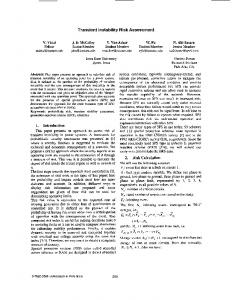
Iso-surfaces of the axial velocity component of unstable modes. The blue colour represents negative values while the red colour represents positive values. m is the azimuthal wave number and k is the axial or stream-wise wave number. The axial wave numbers are chosen to maximize the temporal growth rates of the modes at certain azimuthal wave numbers. . . . . . . . . . . . . . . . . . . . . . . . . . . . . . . . 26

1.3

Vector example of transient growth. The magnitude of f = Φ1 − Φ2 increases before decaying to zero as both Φ1 and Φ2 decay (Schmid 2007). . . . . . . . . . . . . . . . . . . . . . . . . . . . . . . . . . . . 28

1.4

Spiral (left) and bubble (right) breakdown (Lim & Cui 2005). . . . . 29

1.5

Schematic of a typical vortex wake of a transport aircraft in high-lift configuration (flaps deflected). The scale in the downstream direction is compressed by a factor between 5 and 10 (Meunier et al. 2005).

1.6

. 30

(a)-(c) Cross-cut experimental dye visualizations of two laminar corotating vortices, and (d)-(f) vorticity fields obtained by two-dimensional DNS. The snapshots are taken before [(a), (d)], during [(b), (e)] and after [(c), (f)] merging (Meunier et al, 2005).

2.1

. . . . . . . . . . . . . 31

The family of sixth-order one-dimensional Gauss-Lobatto-Legendre Lagrange functions on the domain [−1, 1]. . . . . . . . . . . . . . . . 42

2.2

Structure of the global matrix system. . . . . . . . . . . . . . . . . . 47

3.1

Swirl velocity components for typtical (a) discrete mode, (b,c) potential modes and (d) free-stream mode at azimuthal wave number m = 0, axial wave number k = 10, swirl strength q = 3 and Reynolds number Re = 1000. The real part Re(w) is denoted by solid lines while the absolute value |w| is illustrated by dotted lines. The dashed line r = 1.122 represents the position of the core radius of the Batchelor vortex, corresponding to the maximum azimuthal velocity W = 0.639q (see equation (1.6)). . . . . . . . . . . . . . . . . 59

3.2

Convergence of the spectra of D. The azimuthal and axial wave numbers, Reynolds number and swirl strength are the same as used in figure 3.1. . . . . . . . . . . . . . . . . . . . . . . . . . . . . . . . . 71

3.3

Convergence of the pseudospectra of D. The spectrum is denoted by points while the pseudospectra are represented by lines. The azimuthal and axial wave numbers, Reynolds number and swirl strength are the same as used in figure 3.1. . . . . . . . . . . . . . . . . . . . . 72

3.4

Scaled radial distribution of free-stream modes at various axial wave numbers. The radial wave number is fixed at n = 2π, where n is the radial wave number (see §3.6). The dotted lines r = 1.122, where the azimuthal velocity reaches maxima, represent the core radius of the Batchelor vortex. . . . . . . . . . . . . . . . . . . . . . . . . . . . . . 75

3.5

Ranges of {β∗ , r∗ } for which the twist condition is satisfied (-) or not (×). . . . . . . . . . . . . . . . . . . . . . . . . . . . . . . . . . . . . 79

3.6

Symbol curves with β∗ > 0. “×” marks the points where the twist condition is not satisfied. The arrows indicate the direction in which β∗ or r∗ increases. . . . . . . . . . . . . . . . . . . . . . . . . . . . . . 81

10

3.7

Symbols where the twist condition is satisfied at fixed β∗ and r∗ . The symbols from solution (i) are denoted by “⋄” while symbols from solution (ii) are denoted by ”+”. The arrows indicate the direction in which β∗ or r∗ increases. . . . . . . . . . . . . . . . . . . . . . . . . 82

3.8

Eigenmode at σ = −5.46 − 1.07i in the form of one wave packet. wabs = |w|/maxr |w|. Predicted wave numbers and locations of the wave packets from two solutions are (β∗1 , r∗1 ) = (2.31, 1.53), denoted by the dashed line, and (β∗2 , r∗2 ) = (2.31, 1.43), denoted by the dotted line. . . . . . . . . . . . . . . . . . . . . . . . . . . . . . . . . . . . . 83

3.9

Eigenmode at σ = −3.50 − 5.91i in the form of two wave packets. wabs = |w|/maxr |w|. Predicted wave numbers and locations of the wave packets from two solutions are (β∗1 , r∗1 ) = (1.84, 0.792), denoted by the dashed line, and (β∗2 , r∗2 ) = (1.84, 0.626), denoted by the dotted line. . . . . . . . . . . . . . . . . . . . . . . . . . . . . . . . . 84

3.10 Integration contour of inverse Laplace transformation. . . . . . . . . . 88 3.11 Three typical eigenmodes of the operator Dm=1 . . . . . . . . . . . . . 90 4.1

Leading pseudospectra at various axial wave numbers. The points represent the spectrum while the solid lines represent the pseduospectra corresponding to ǫ = 10−2 , ǫ = 10−3 and ǫ = 10−4 from outer to inner. The contour lines around the discrete eigenvalues correspond to ǫ = 10−3 . . . . . . . . . . . . . . . . . . . . . . . . . . . . . . . . . 94

4.2

Local transient energy growth.

. . . . . . . . . . . . . . . . . . . . . 97

4.3

Absolute values of optimal perturbations and outcomes constructed from the whole spectrum, continuous spectrum and discrete spectrum at k = 1, q = 3 and τ = 680. The values are normalized by the energy norm. . . . . . . . . . . . . . . . . . . . . . . . . . . . . . . . . . . . 98

11

4.4

Radial distributions of the radial velocity component of the optimal initial perturbation (t = 0) and its outcome (t = 60). Here the time interval used is τ = 60 and the azimuthal wave number is m = 1. . . . 99

4.5

Computational mesh for transient growth calculation and DNS in the aximuthally decomposed domain. . . . . . . . . . . . . . . . . . . . . 102

4.6

(a): Optimal energy growth and three transient responses at q = 2. (b): Development of energy of separated velocity components from optimal perturbation at τ = 60. (c): Dominant axial wave numbers of optimal perturbations. (d): Energy radii of the optimal perturbations.

4.7

. . . . . . . . . . . . . . . . . . . . . . . . . . . . . . 105

Illustration of the optimal perturbation and outcome at τ = 60 and q = 2. The blue colour represents negative values of the azimuthal vorticity and the red colour represents the positive values. . . . . . . 106

4.8

Non-linear outcome of the optimal perturbation at t = τ = 60 and q = 2. The value of iso-surfaces are -0.2. The contour levels are from -0.4 to 1 and the blue colour represents negative values of the azimuthal vorticity while the red colour represents the positive values. 108

4.9

Computational mesh for the validation, transient growth calculation and DNS in the axially decomposed global analysis.

. . . . . . . . . 110

4.10 (a) Optimal energy growth and transient responses of three optimal perturbations. (b) Radius of the structure of the optimal perturbations.

. . . . . . . . . . . . . . . . . . . . . . . . . . . . . . . . . . . 111

4.11 Contours of the streamwise vorticity in the linearized evolution of the optimal perturbation. The black circle denotes the vortex core, r = 1.121. The blue colour represents negative values while the red colour represents positive values. The same contour levels are used in all subfigures. . . . . . . . . . . . . . . . . . . . . . . . . . . . . . . 113

12

4.12 Contours of the streamwise vorticity in the DNS of the Batchelor vortex initially perturbed by the optimal perturbation. The contour levels range from 0.2 to 3 and the same levels are used in all the subplots. The red colour represents higher contour levels while the blue colour represents lower levels. . . . . . . . . . . . . . . . . . . . . 114 4.13 Vibration of the vortex centre driven by optimal perturbations. The arrow represents the direction of vibration.

. . . . . . . . . . . . . . 115

4.14 Energy of perturbations in DNS and LNS. . . . . . . . . . . . . . . . 116 5.1

Spiral breakdown of the Batchelor vortex at q = 0.8, visualized using iso-surfaces of λ2 = −0.4, coloured by the axial velocity component. . 121

5.2

Bubble-type breakdown at q = 2, visualized using contours of azimuthal vorticity of the perturbation on the plane θ = 0 with the same contour levels on all subfigures (left) and iso-surfaces of azimuthal vorticity− 0.2, −0.3, −0.4 from top to bottom (right).

5.3

. . . . . . . . . . . . . . 123

Reduction of the ratio of non-axisymmtric energy (Em6=0 ) and axisymmetric energy (Em=0 ) at t = 35 and q = 2. . . . . . . . . . . . . . 123

5.4

DNS of the Batchelor vortex perturbed by a helical unstable mode at m = 4 and k = −2.2. (a) Iso-surface of λ2 = −0.00004 for the initial perturbation. (b) Iso-surface of λ2 = −0.4 for the outcome at t = 35 with fixed inflow boundary conditions. (c) Development of energy in the LNS (dashed line) and DNS (solid lines) using time dependent inflow boundary conditions. . . . . . . . . . . . . . . . . . . . . . . . 124

13

5.5

Viscous diffusion effects on vortex breakdown, visualized using isosurfaces, coloured by the axial velocity component. (a), (b): λ2 = −0.4, q = 0.8 and t = 35 using fixed inflow boundary conditions and decaying time-dependent boundary conditions. (c), (d): Azimuthal vorticity −0.2 at q = 2 and t = 60 using fixed inflow boundary conditions and decay time-dependent boundary conditions. The light grey tube illustrates the vortex radius. . . . . . . . . . . . . . . . . . 126

5.6

Effects of external favourable pressure gradients on the vortex breakdown. (a), (b) Iso-surfaces of λ2 = −0.4 at q = 0.8 and t = 35 with and without pressure gradients, coloured by the axial velocity component. (c), (d) Contours of azimuthal vorticity at q = 2 and t = 35 with and without pressure gradients. . . . . . . . . . . . . . . . . . . 127

6.1

Mesh used in the base flow calculation, transient growth and DNS studies for both individual vortex and co-rotating vortex pair simulations.

6.2

. . . . . . . . . . . . . . . . . . . . . . . . . . . . . . . . . . 131

Contours showing the development of axial vorticity in the co-rotating vortex base flow from the initial condition as described in equations (6.1)-(6.3). The Reynolds number is Re = 100, the vortex distance b = 6 and the swirl strength q = 3. The contour levels range from 0 to 3.5 and the same levels are used in all subplots. . . . . . . . . . . . 133

6.3

Vorticity contours of two major instabilities for an individual vortex: (a) helical instability at (Re, q, k) = (1000, 0.8, 1.7) and (b) viscous centre instability at (Re, q, k) = (3000, 2, 0.27). The asymptotic growth rates are σ = 0.323 and σ = 0.00917, respectively. . . . . . . . 134

6.4

Contours of optimal energy growth for the individual vortex and corotating vortices at Re = 100 and q = 3. . . . . . . . . . . . . . . . . 135

6.5

Optimal energy growth and transient responses of the individual vortex and the co-rotating vortex pair at Re = 100, q = 3 and k = 0. . . 137

14

6.6

Vorticity contours of optimal perturbations and outcomes of an individual vortex and a co-rotating vortex pair at (Re, q, k) = (100, 3, 0). The same contour levels are used on the left and right plots. . . . . . 138

6.7

Axial vorticity contours of optimal perturbations and outcomes in an individual vortex and a co-rotating vortex pair at (Re, q, k) = (100, 3, 0.75). The same contour levels are used for the initial perturbations and outcomes. . . . . . . . . . . . . . . . . . . . . . . . . . . 141

6.8

Optimal growth of the individual vortex and co-rotating vortex pair at (a) (Re, q, k) = (1000, 0.8, 1.7) where a helical instability with growth rate σ = 0.323 exists in the individual vortex and (b) (Re, q, k) = (3000, 2, 0.27), where a viscous centre instability with growth rate σ = 0.00917 exists in the individual vortex. . . . . . . . . . . . . . . . 142

6.9

Vorticity contours of optimal perturbations of an individual vortex and a pair of co-rotating vortices when the individual vortex is helically unstable at (Re, q, k) = (1000, 0.8, 1.7). . . . . . . . . . . . . . . 143

6.10 Vorticity contours of optimal initial perturbations of an individual vortex and a pair of co-rotating vortices when the individual vortex has viscous centre instability at (Re, q, k) = (3000, 2, 0.27). . . . . . . 145 6.11 Vorticity contours of the DNS of the vortex pair perturbed by the optimal perturbation at τ = 5 and (Re, q, k) = (100, 3, 0). The relative energy of the perturbation is 10−4. The unperturbed counterpart is shown on the left to highlight the difference. The same contour levels are used as in figure 6.2. . . . . . . . . . . . . . . . . . . . . . . . . . 147 6.12 Vorticity contours of the DNS of the vortex pair perturbed by the optimal perturbation at τ = 39 and (Re, q, k) = (100, 3, 0). The relative energy of the perturbation is 10−4. The unperturbed counterpart is shown on the left to highlight the difference. The same contour levels are used as in figure 6.2. . . . . . . . . . . . . . . . . . . . . . . . . . 148 6.13 Effect of perturbation energy levels on the merging process. . . . . . . 148 15

6.14 Energy growth of the optimal perturbation at different initial perturbation energy levels. In the non-linear evolution, the perturbation is obtained after subtracting the unperturbed base flow from the DNS outcomes. . . . . . . . . . . . . . . . . . . . . . . . . . . . . . . . . . 149 6.15 Energy growth of perturbations at different axial modes in DNS and LNS, where (Re, q, k) = (100, 3, 0.75).

. . . . . . . . . . . . . . . . . 150

6.16 Iso-surfaces of axial voriticity=1 in DNS at (Re, q, k) = (100, 3, 0.75), coloured by the axial velocity. . . . . . . . . . . . . . . . . . . . . . . 151 7.1

Computational mesh and boundaries. . . . . . . . . . . . . . . . . . . 162

7.2

The gain G VS τ and ω at (Re, a, q) = (100, 0.5, 0.8). . . . . . . . . . 165

7.3

Velocity components of optimal boundary perturbations at q = 0.8. The boundary perturbation has been normlized so that [uc , uc ] = 1.

7.4

166

Contours of the axial velocity component of the final conditions of the optimal inflow boundary conditions at t = 15. The boundary perturbation has been normlized so that [uc , uc ] = 1. The same contour levels are used on all the subfigures, that is [-0.5,0.5]. The red colour represents positive values while the blue colour represents the negative values. . . . . . . . . . . . . . . . . . . . . . . . . . . . . 167

7.5

Energy growth VS τ and ω at (Re, a, q) = (100, 0.5, 3). . . . . . . . . 168

7.6

Velocity components of optimal boundary perturbations at q = 3. The boundary perturbation has been normlized so that [uc , uc ] = 1.

7.7

169

Contours of the axial velocity component of the final conditions of optimal inflow boundary conditions at t = 15. The boundary perturbation has been normlized so that [uc , uc ] = 1. The same contour levels are used on all the subfigures, that is [-0.5,0.5]. The red colour represents positive values while the blue colour represents the negative values. . . . . . . . . . . . . . . . . . . . . . . . . . . . . . . . . . 170

16

7.8

Contours of the azimuthal velocity component of optimal initial perturbations obtained at (q, a, τ ) = (3, 0, 15) (left) and their outcomes at t = 15 (right). . . . . . . . . . . . . . . . . . . . . . . . . . . . . . 170

17

List of Tables 2.1

Test functions vj (x) used in the method of weighted residuals and the corresponding numerical method produced. . . . . . . . . . . . . . . . 41

2.2

Implicit and explicit weights αq , βq in the time discretization scheme.

3.1

Validation against published results and theoretical values. M is

51

the number of Chebyshev polynomials, R is the radial length of the domain and σ is the growth rate. Left: Leading unstable discrete eigenvalue at azimuthal wave number m = −3, swirl strength q = 0.761, axial wave number k = 1.659 and Reynolds number Re = 1000. Right: Leading eigenvalue in the continuous spectrum at m = 0, q = 3, k = 10 and Re = 1000. The theoretical value of the leading continuous eigenvalue −k 2 /Re = −0.1 is obtained in section 3.6. . . . 69 4.1

Comparison of the growth rate of a viscous centre unstable mode at Re = 14000, q = 2, m = −1 and k = 0.268 obtained using the present method and other published methods. . . . . . . . . . . . . . . . . . . 103

4.2

Convergence of the growth rate on the spectral/hp element polynomial order. . . . . . . . . . . . . . . . . . . . . . . . . . . . . . . . . . 103

4.3

Validation of the numerical method and convergence of the growth rate of the Batchelor vortex on the polynomial order P at swirl strength q = 0.761, axial wave number k = 1.658 and azimuthal wave number m = −3. . . . . . . . . . . . . . . . . . . . . . . . . . . 110

6.1

Validation and convergence of the asymptotic growth rate σ of a perturbation to an individual Batchelor vortex with respect to the spectral/hp element polynomial order P . . . . . . . . . . . . . . . . . 132

7.1

Convergence of the growth with respect to P at (Re, q, a, τ, ω, m) = (100, 0.8, 0, 10, 0, 3). . . . . . . . . . . . . . . . . . . . . . . . . . . . . 162

7.2

Convergence of the growth at (Re, q, a, τ, ω, m) = (1000, 2, 0, 10, 0, 0). 163

19

Chapter 1 Introduction 1.1

Modeling a vortex

1.1.1

Definition of a vortex

The definition of a vortex is a topic of much discussion in fluid mechanics. The common intuitive features of a vortex are a pressure minimum, closed or spiralling streamlines, and iso-surfaces of constant vorticity. Jeong & Hussain (1995) have proposed a definition of a vortex as a pressure minimum in the absence of unsteady straining and viscous effects. Following the notations of Jeong & Hussain (1995), the Navier-Stokes (NS) equations can be expressed as 1 ai = − p,i + νui,kk , ρ

i = 1, 2, 3,

(1.1)

where ai =

Dui , Dt

p,i =

∂p ∂xi

and

ui,kk =

∂ 2 ui ∂ 2 ui ∂ 2 ui + + . ∂x21 ∂x22 ∂x23

Taking the gradient of equation (1.1) to obtain: 1 ai,j = − p,ij + νui,jkk , ρ

i, j = 1, 2, 3.

(1.2)

It is possible to decompose ai,j into symmetric and anti-symmetric contributions, DSij DΩij (1.3) ai,j = + Ωik Ωkj + Sik Skj + + Ωik Skj + Sik Ωkj , Dt Dt | {z } | {z } symmetric

where

1 Sij = 2

∂ui ∂uj + ∂xj ∂xi

antisymmetric

and

1 Ωij = 2

∂ui ∂uj − ∂xj ∂xi

.

Here, Sij is symmetric and Ωij is anti-symmetric. Equation (1.2) can then be written as: 1 ai,j = − p,ij + ν(Sij,kk + Ωij,kk ). ρ

(1.4)

Equating the symmetric parts of equation (1.3) and (1.4) to obtain: 1 DSij − p,ij + νSij,kk = + Ωik Ωkj + Sik Skj . ρ Dt Finally, removing the unsteady and viscous terms to reach: 1 − p,ij = Ωik Ωkj + Sik Skj = (S 2 + Ω2 )ij . ρ The occurrence of a local pressure minimum in a plane requires two negative eigenvalues of p,ij (Jeong & Hussain 1995). Since the pressure tensor is symmetric and real, its eigenvalues are real. Assuming the eigenvalues are λ1 , λ2 , and λ3 and λ1 ≥ λ2 ≥ λ3 , the existence of a pressure minimum requires that the second eigenvalue must be negative. Therefore a coherent vortex structure is equivalent to an iso-surface of constant negative λ2 .

1.1.2

The Batchelor vortex

The Batchelor vortex is an approximated solution to the NS equations under the boundary-layer-type approximation obtained by Batchelor (1964). In terms of dimensional variables, the axial, radial and azimuthal velocity components of the Batchelor vortex represented in the cylindrical coordinates (z ∗ , r, θ) can be written

21

as:

    

U ∗ (r ∗ ) = U∞ +

∗ 2 W0 e−(r /R) , (R/R0 )2

V ∗ (r ∗ ) = 0,     W ∗ (r ∗ ) = qW 1−e−(r∗ /R)2 , 0 r ∗ /R0

(1.5)

where the dimensional variables are indicated by a ∗ superscript, z ∗ denotes the steamwise coordinate, U∞ is the free-stream axial velocity, q is the swirl strength measuring the ratio between the maximum tangential velocity and core velocity, and p R(t) = R02 + 4νt∗ is a measure of the core size, with R0 representing the initial

core size and ν denoting the viscosity.

It is convenient to introduce non-dimensional variables (without a ∗ superscript) by selecting R0 as the length scale, W0 as the velocity scale and R0 /W0 as the time scale. In terms of non-dimensional variables, the velocity components in equation 1.5 becomes:    U(r) = a +  

√

1 e−(r/ 1+4t/Re

V (r) = 0,  √    W (r) = q 1−e−(r/ 1+4t/Re)2 , r

1+4t/Re)2

, (1.6)

where a = U∞ /W0 denotes the external free-stream axial velocity. It has been noted by Lessen, Singh, & Paillet (1974) that the translation and inversion of the axial velocity does not affect the instability of the Batchelor vortex – it only affects the frequency, leaving the growth rates unchanged, so a = 0 is adopted in this work unless otherwise stated. Re denotes the Reynolds number, defined as Re = W0 R0 /ν. p 1 + 4t/Re represents In this work, Re is set to be 1000 unless otherwise stated.

the viscous diffusion of the vortex core. When considering the instability or nonnormality of the vortex, the viscous diffusion factor is commonly neglected and the base flow is considered to be time-independent, but, in the non-linear analysis, this factor has a significant impact on the bubble-type breakdown. The pressure field can be determined from dP/dr = [W (r)]2 /r (Abid 2008). A typical profile of the Batchelor vortex is shown in figure 1.1.

22

3

2

2

1

1

0

0

r

r

3

−1

−1

−2

−2

−3 0

a 0.5

u

1

−3

1.5

−0.5

(a) Axial velocity

0 w

0.5

(b) Azimuthal velocity

Figure 1.1: Velocity profiles of the Batchelor vortex at q = 0.8 and a = 0.5. The radial velocity is zero and is not shown here. In this thesis, the Bachelor vortex is adopted as the mathematical model of the vortex since this profile is widely used in the stability studies of vortex flow and it is convenient to validate the methodology and discretization against published data.

1.1.3

Other vortex models

There are several other well-documented models of vortex flow, such as the LambOseen vortex, the Burgers vortex, the Rankine vortex and so on. The profiles of these models are summarized below. a) The Lamb-Oseen vortex. This model is named after Horace Lamb and Carl Wilhelm Oseen (Saffman 1992). At co-flow parameter a = 0 and infinitely large swirl number q, the Batchelor vortex is simplified to the Lamb-Oseen vortex, whose velocity components in a cylindrical coordinate system are: U(r) = 0,

V (r) = 0

and

W (r) =

i √ 1h 2 1 − e−(r/ 1+4t/Re) . r

b) The Burgers vortex. This is a combination of the Lamb-Oseen vortex and a 23

uniform axial velocity, or a co-flow parameter a (Wang & Rusak 1997): U(r) = a,

V (r) = 0

√ 1 2 W (r) = [1 − e−(r/ 1+4t/Re) ]. r

and

c) The Rankine vortex. This model is named after its creator, William John Macquorn Rankine (Acheson 1990). It is defined as a vortex flow with uniform axial velocity: U(r) = a,

and

V (r) = 0

and

W (r) =

  

ωr,

0 ≤ r ≤ R0

ωR02 /r, R0 ≤ r

where ω is the angular speed at the vortex centre and R0 is the vortex core size (Wang & Rusak 1997). d) The Grabowski profile (Grabowski & Berger 1976). After non-dimensionalizing the radial coordinate by the characteristic core radius and the velocity components by the freestream axial velocity, the Grabowski profile can be expressed as:   α + (1 − α)r 2(6 − 8r + 3r 2 ) 0 ≤ r ≤ 1 U=  1 1≤r V =0   W = 

Sr(2 − r 2 ) 0 ≤ r ≤ 1 S/r

1≤r

Here, S represents the azimuthal velocity at the edge of the core and α denotes the ratio of the velocity at the axis to the velocity in the free-stream.

1.2

Linear stability analysis of vortex flow

Depending on the radial distribution, the linear eigenmodes of the Batchelor vortex can be classified into three broad categories: a) Discrete modes. These modes correspond to a discrete spectrum of the linearized evolution operator of perturbations. Discrete modes have been investigated by Obrist & Schmid (2003a) in the free-stream of a leading-edge boundary layer flow, 24

where it is observed that they decay exponentially in the wall-normal direction. More recently, an unstable viscous ring discrete mode, which is spatially concentrated near a particular radius corresponding to a double critical point of the invisicd equation, is reported by Le Dizés & Fabre (2010). In this work the discrete mode of the Batchelor vortex is observed to decay exponentially or super-exponentially in the radial direction. Discrete modes have been extensively studied in both invisicid and viscous conditions since Rayleigh (1916) proposed his famous stability criterion. To date, all the reported unstable modes of the Batchelor vortex are discrete modes. There are two typical unstable discrete modes: inviscidly unstable modes and viscously unstable modes. Inviscid helical modes have exponential temporal growth rates, which increase to finite values as Re → ∞. Helical modes are known to be present for swirl strength 0 < q < 2.3. These modes are very unstable at small q and become very weak when q > 1.6 (Lessen, Singh, & Paillet 1974; Lessen & Paillet 1974; Heaton 2007a). The most unstable inviscid helical modes at azimuthal wave number m = 1, 2, 3 are shown in figures 1.2(a), (b), (c). Viscous modes have exponential growth rates, which decrease to zero as Re → ∞. Viscosity was first found to stabilise some helical modes (Lessen & Paillet 1974). The first purely viscous unstable modes were found by Khorrami (1991), and they only exist for azimuthal wave numbers m = 0 and |m| = 1. More recently, a centre mode at high Reynolds number was introduced by Fabre & Jacquin (2004). The structure of this centre mode is concentrated along the vortex centreline, and the growth rate is much smaller than the helical modes, typically 10−2 or less. This mode exists for all values of q. A typical viscous centre mode is shown in figure 1.2(d). b) Potential modes. These correspond to a continuous spectrum. Potential modes have also been investigated in the potential flow region around swept bluff bodies (Obrist & Schmid 2010), where a spanwise velocity component exists due to 25

(a) Inviscid, m = −1, k = 0.3, q = 0.32

(b) Inviscid, m = −2, k = 1.2, q = 0.7

(c) Inviscid, m = −3, k = 1.7, q = 0.79

(d) Re = 14000, m = −1, k = 0.268, q = 2

Figure 1.2: Iso-surfaces of the axial velocity component of unstable modes. The blue colour represents negative values while the red colour represents positive values. m is the azimuthal wave number and k is the axial or stream-wise wave number. The axial wave numbers are chosen to maximize the temporal growth rates of the modes at certain azimuthal wave numbers. the sweep angle and this has a similar effect to the azimuthal velocity in the vortex flow in generating potential modes. Obrist & Schmid (2003a) have demonstrated analytically that potential modes decay algebraically in the radial direction in the leading-edge boundary layer flow. In the context of vortex flow discussed in the present work, the potential modes are also observed to decay algebraically through inspecting the radial distribution of these modes. Potential modes are asymptotically stable, but a linear combination of them produces significant transient growth (Obrist & Schmid 2003b). It is shown in this work that the transient growth of the Batchelor vortex reported by Heaton & Peake (2007) is associated with the potential modes. c) Free-stream modes. These are a limit condition of the potential modes when the radial decay rate tends to zero. The corresponding spectrum of these free-stream modes is similar to the well-documented “continuous spectrum” in the boundary layer flow. Free-stream modes are the only modes surviving in the far free stream.

26

Most of the published work on free-stream modes/spectra is related to the continuous spectrum of the one-variable Orr-Somerfeld (O-S) equation in boundary layer flow. The existence of free-stream modes of the O-S equation for a Blasius boundary layer was conjectured by Jordinson (1970) and confirmed both by a numerical approach (Mack 1976) and analytical expressions (Gustavsson 1979; Grosch & Salwen 1978). It was found that the free-stream modes are small in the boundary layer and oscillatory in the free stream. Zaki & Saha (2009) have demonstrated that free-stream modes with small axial wave numbers penetrate the boundary layer and therefore provide a mechanism to introduce free-stream turbulence into the boundary layer. The free-stream spectrum however has not been very actively investigated in vortex flow whose governing equations cannot be reduced to a single-variable equation. Fabre et al. (2006) noted that there would be a free-stream spectrum in the vortex flow, but they did not provide a mathematical investigation of this observation.

1.3

Non-normality analysis of vortex flow

Hydrodynamic stability theory has focused on the leading eigenvalues/least stable eigenmodes of the governing linearized operator and discards the short-time perturbation dynamics and its consequence on scale selection and transition scenarios. When the asymptotic growth rate is small, the time-asymptotic fate, as well as the shape of the least stable mode, may be irrelevant to the overall perturbation dynamics, as this limit may never, or only under artificial conditions, be reached (Schmid 2007). For example, the maximum growth rate of the viscous centre unstable modes in the parameters introduced above is about 0.02. At this growth rate, it takes more than 100 time units to grow by one order of magnitude. However, some particular perturbations, in the form of a combination of eigenmodes, grow by one order of magnitude in less than 10 time units. Figure 1.3 schematically illustrates the difference between short-time and asymptotic dynamics. When both vectors Φ1 and Φ2 decay, the sum of them, f grows owing to the non-normality of Φ1 and Φ2 . 27

This figure indicates that it is possible for some particular perturbations to grow significantly before eventually decaying when all the eigenmodes are stable.

Figure 1.3: Vector example of transient growth. The magnitude of f = Φ1 − Φ2 increases before decaying to zero as both Φ1 and Φ2 decay (Schmid 2007). To quantitatively describe the short-time dynamics owing to non-normality of the eigenmodes, the concept of transient energy growth is introduced. Transient growth over a finite time interval is defined as the maximum energy growth over all the possible initial perturbations. There are three main approaches to calculating the transient growth: a) Singular value decomposition. When the matrix of the discretized governing operator is available, usually in a local analysis, the optimal energy growth is the square of the largest singular value of the matrix. This method is used in the local studies in this work. b) Arnoldi method. In more general cases, the matrix of the discretized operator is not available. In this condition, a random initial perturbation is evolved forwards through the linearized NS (LNS) equations and then backwards through the adjoint equations, which is obtained through integration by parts. Finally an Arnoldi method is adopted to calculate the largest eigenvalue of the joint operator, which is the optimal energy growth. This method is used in the global studies in this work. c) Optimization method. A Lagrangian function consisting of the cost function 28

(energy growth to optimize) and penalty terms (restraints to satisfy the LNS equations). This method is used in the sensitivity studies in this work to validate the optimization methodology.

1.4

Vortex breakdown

Vortex breakdown is defined as “an abrupt change in the structure with a very pronounced retardation of the flow along the axis and a corresponding divergence of the stream surfaces near the axis” (Hall 1972). This vortex breakdown definition is adopted in this report, as opposed to the stricter definition of Leibovich (1978), where a stagnation point is also required. According to the nature of the breakdown, it can be broadly categorised into two types, spiral breakdown and bubble breakdown, as illustrated in figure 1.4 (Lim & Cui 2005).

Figure 1.4: Spiral (left) and bubble (right) breakdown (Lim & Cui 2005). Spiral breakdown is a non-axisymmetric development of the disturbance, while the bubble breakdown is often characterized by its axisymmetric nature, but it also has non-axisymmetric structures downstream of the stagnation point (Ruith et al. 2003). Under the axisymmetric assumption, bubble breakdown bifurcating from columnar flows have been found using a stagnation model (Wang & Rusak 1997). In the context of the Batchelor vortex, spiral breakdown resulting from the helical instabilities has been observed by Broadhurst (2007) and is confirmed in this work, while the bubble-type breakdown is found to be induced by the viscous diffusion of the velocity components in this work.

29

1.5

Vortex interactions

Large aircraft are known to generate multiple trailing vortex systems, whose strength scales with aircraft size. In the near field, the vortex sheet quickly rolls up and detaches from the wing tips and outer flaps to form a set of discrete co-rotating vortices along each semi-span, which subsequently merge and form a pair of counterrotating vortices downstream of the wing over a distance of 5-10 wing spans (Meunier, Le Dizés, & Leweke 2005), as illustrated in figure 1.5. Such vortex systems persist over a long time before finally diffusing, and impose potentially dangerous rolling moments on following aircraft. Airport safety regulations impose a minimum distance between aircraft in order to avoid such danger.

Figure 1.5: Schematic of a typical vortex wake of a transport aircraft in highlift configuration (flaps deflected). The scale in the downstream direction is compressed by a factor between 5 and 10 (Meunier et al. 2005). The importance of vortex interaction and merging in the co-rotating vortex system has resulted in a large number of papers dealing with the mechanism of merging and perturbation propagation in this process. The vortex merging process is illustrated in figure 1.6. Meunier & Leweke (2005) found in their experimental research that three-dimensional effects, in the form of elliptic short-wave instabilities arising in the initial co-rotating flow cause significant changes to the merging process, such as earlier merging and larger final vorex cores. A similar transient growth effect on

30

Figure 1.6: (a)-(c) Cross-cut experimental dye visualizations of two laminar co-rotating vortices, and (d)-(f) vorticity fields obtained by two-dimensional DNS. The snapshots are taken before [(a), (d)], during [(b), (e)] and after [(c), (f)] merging (Meunier et al, 2005).

31

the acceleration of the merging process is described in this work. Another vital factor in the merging process, the merging condition or threshold, has been proposed as a function of the ratio between the vortex core size and the separation distance. Various investigations find that the value of the ratio ranges from 0.22–0.326 (Meunier, Ehrenstein, Leweke, & Rossi 2002; Le Dizés & Verga 2002; Cerretelli & Williamson 2003). In this work, the ratio 0.23 is used as the merging threshold, as used by Roy et al. (2008) and Le Dizés & Laporte (2002) in their stability studies. The study of the linear dynamics of the vortex system has been primarily concerned with the asymptotic instabilities of the system. The instabilities of corotating and counter-rotating vortex pairs have also been extensively studied. The theoretical work of Crow (1970) on a pair of counter-rotating vortex filaments predicted the existence of a long-wavelength symmetric (with respect to the plane separating the two vortices) instability with a wave length of five to ten times of the vortex separation distance. This prediction had been confirmed in the work of Donnadieu et al. (2009). A short-wave elliptic instability was theoretically described by Moore & Saffman (1975) as the resonant interaction between the strain and Kelvin waves with azimuthal wavenumbers m = −1 and m = 1. This elliptic instability has been well documented by Kerswell (2002) and confirmed in the co-rotating vortex pair flow (Le Dizés & Laporte 2002; Meunier & Leweke 2005). Lacaze et al. (2007) demonstrated that as the axial flow is increased, the elliptic instability involving resonant Kelvin modes with azimuthal wave numbers m = −1 and m = 1, the most unstable instability in the absence of axial flow, becomes damped. This damping of instabilities is owing to the damping of one of the resonant Kelvin modes due to the appearance of a critical layer while other combinations of resonant Kelvin modes become progressively unstable. Recently, a new oscillatory elliptic instability involving Kelvin waves with azimuthal wavenumbers m = 0 and |m| = 2, whose growth rates have imaginary parts, has been examined by Donnadieu et al. (2009), who also investigated the transient growth of a counter-rotating vortex pair. Linearized dynamic analysis of the vortex system has previously focused on the 32

quasi-steady instability by freezing the base flow, obtained by evolving the linear summation of two vortex mathematical models over a short time interval for each vortex to equilibrate with the other. This base flow is then taken to be quasistationary and assumed to satisfy the NS equations. In the co-rotating vortex system, the Coriolis terms are added to the governing equation (Roy, Schaeffer, Le Dizés, & Thompson 2008) while in the counter-rotating case, the advection velocity is subtracted from the base flow (Donnadieu, Ortiz, Chomaz, & Billant 2009). In this approach, based on quasi-stationary simplification of the base flow, viscous diffusion, vortex interaction and merging are neglected. However, on the time scale t = O(Re) where the base flow diffusion becomes non-negligible, eigenmodes cease to be a valid approximation of the solution (Fabre, Sipp, & Jacquin 2006). Considering the importance of vortex interactions and vortex core expansions in the dynamics of vortex systems, it is necessary to take into account the time-dependence of the base flow and conduct dynamic analysis over the whole process of the vortex interaction until merging completes. Transient growth analysis is an ideal tool to study this problem but very limited attention has been paid to the finite-time dynamics of vortex system in the unsteady evolution process. In this work, a co-rotating vortex pair is adopted as an example vortex system and then transient dynamics in the expansion-merging process are investigated. The choice of co-rotating rather than counter-rotating vortex pair means that the individual vortices undergo rotation around their centroid rather than parallel translation, which could require a much larger computational domain. In addition, most of the previous papers on the dynamics of vortex pairs are concerned with vortex systems consisting of individually stable vortices. The interaction of the individual instabilities with the system instabilities has not been fully understood. In this work, the dynamics of vortex pairs consisting of individually unstable vortices are investigated and compared with the dynamics of the individual vortex in order to fill this gap.

33

1.6

Scope of the thesis

This thesis analyses the hydrodynamic instability and non-normality of the vortex flow and focuses on the behavior of the continuous spectra/modes. The remainder of this thesis is organized as follows: In Chapter 2, the numerical methods used in global analysis and direct numerical simulations, including the spectral/hp element method, velocity-correction scheme and Fourier decomposition in the azimuthal direction are briefly introduced. In Chapter 3, the perturbation in the vortex is Fourier decomposed in both axial and azimuthal directions and then the localized LNS equations are discretized using a modified Chebyshev polynomial method. The spectrum of the governing operator is divided into three parts: a free-stream spectrum, a potential spectrum and a discrete spectrum. The first two spectra are continuous and this continuity is verified by the convergence of the spectrum, convergence of the pseudospectrum and a wave-packet pseudomode method. The two continuous spectra are always asymptotically stable while the discrete spectrum can be unstable for some combinations of parameters. In Chapter 4, the non-normality of the eigenmodes in the vortex flow is investigated. The localized transient energy growth is obtained through singular value decomposition of the linearized operator, while the global transient growth is calculated by a matrix-free Arnoldi method. The physical relevance of the optimal perturbations are studied through direct numerical simulations (DNS) of the vortex flow initially perturbed by the optimal perturbations. In Chapter 5, the spiral and bubble-type vortex breakdown are investigated. The development of columnar flow, initially seeded by helical unstable modes into spiral breakdown, is confirmed. The effects of viscous diffusion and external pressure gradients on the bubble-type breakdown are analyzed. In Chapter 6, the dynamics of a co-rotating vortex pair is studied. The viscous diffusion and vortex merging processes are taken into consideration so that the base flow is time-dependent but not periodic. Three typical vortex pairs are considered:

34

vortex pairs consisting of asymptotically stable vortices, helically unstable vortices and viscous centre unstable vortices. In Chapter 7, an augmented Lagrangian function is built, firstly to calculate the optimal initial conditions to validate the method, and then to compute the optimal inflow boundary perturbation which generates maximum energy over a fixed time interval. The second optimization is close to the concept of flow control and sensitivity.

35

Chapter 2 Numerical Discretization Assuming the fluid to be Newtonian and the flow incompressible, the relevant equations of motion for the primitive variables (velocities, pressure), denoted by a superscript ∗, are the incompressible NS equations. In the cylindrical system (z ∗ , r ∗, θ) where z ∗ represents the stream-wise coordinate, the NS equations can be expressed as 1 ∂t∗ u∗ = −(u∗ · ∇)u∗ − ∇p∗ + ν∇2 u∗ , ρ

with

∇ · u∗ = 0,

(2.1)

where u∗ (z ∗ , r ∗ , θ, t∗ ) is the velocity field, p∗ (z ∗ , r ∗ , θ, t∗ ) is the pressure, ρ is the density and ν is the viscosity. The equations for non-dimensionalized variables (without superscript ∗) are: ∂t u = −(u · ∇)u − ∇p +

1 2 ∇ u, Re

with

∇ · u = 0,

(2.2)

where r = r ∗ /L, z = z ∗ /L, t = t∗ u∞ /L, u(z, r, θ, t) = (u, v, w)(t) = u∗ /u∞ , p = (p∗ − p∞ )/ρu2∞ and Re = u∞ L/ν. Here L, u∞ and p∞ are characteristic length, velocity and pressure respectively. In this work, equations (2.2) are Fourier decomposed in the θ direction so as to transform the 3D equations to a set of 2D problems with various azimuthal wave numbers (Blackburn & Sherwin 2004). Each set of 2d equations is then spatially discretized using a spectral/hp element method (Karniadakis & Sherwin 2005) and

temporally discretized using a velocity-correction scheme (Karniadakis, Israeli, & Orszag 1991). The three essential techniques — spectral/hp element method (§2.1), velocitycorrection scheme (§2.2) and Fourier decomposition in θ (§2.3) — are briefly introduced in this chapter.

2.1

Spectral/hp element method

This section starts by discussing the basic concept of the spectral/hp element discretization (§2.1.1), followed by the construction of local operations defined on a single element (§2.1.2) and global operations defined on a multi-elemental domain (§2.1.3). Finally the complementation of this method on a basic Helmholtz equation is introduced (§2.1.4). For a complete reference of this subject, the interested reader should refer to the textbook by Karniadakis & Sherwin (2005).

2.1.1

Concepts of the spectral/hp element method

The concept of spectral/hp element method (§2.1.1.3) is a combination of the finite element method (§2.1.1.1) and the classic spectral method (§2.1.1.2). These numerical methods can be constructed in the weighted residual scheme by choosing appropriate weight functions (§2.1.1.4). 2.1.1.1

Finite element method

The basic idea of the finite element method is to divide the physical domain Ω into a set of sub-domains (or elements) Ωi , and then locally approximate the solution using a previously chosen expansion basis, which usually consists of low-order functions such as linear or quadratic polynomials. Instead of satisfying the differential equations directly, the approximated solution is substituted into the integrated form of the equation over Ω and a Galerkin formulation is typically used to transfer the resid-

37

ual equation into a system of ordinary equations. This weighted residual method will be described in detail in §2.1.1.4. The finite element method converges by refining the subdivision of the domain (mesh refinement), called h-type refinement. The error in the numerical solution decays algebraically by refining the mesh, that is, introducing more elements while keeping the order of the interpolating polynomial fixed. According to remarks made by Zienkiewicz (1975), Oden (1991) and Jiang (1998), the main features of the finite element method can be summarized as: (1) Arbitrary geometry. The finite element method is essentially independent of the geometry of the computational domain. It can be applied to domains of complex shapes and with quite arbitrary boundary conditions. (2) Unstructured meshes. In finite element analysis a global coordinate transformation is not needed. Finite elements can be placed anywhere in physical domains. 2.1.1.2

Classic spectral method

The classic spectral methods use a single expansion of a function u(x) throughout the domain: δ

u(x) ≈ u (x) =

P X

uîφi (x),

(2.3)

i=0

where φi(x) are the basis functions (or trial functions). The approximated function in expanded form uδ (x) is then substituted into the differential equations to compute the unknown coefficients uî . There are a number of different schemes for minimising the residual of the discretized governing equations. The spectral method can therefore be broadly classified into two categories: the pseudo-spectral or collocation methods and the modal or Galerkin methods. The collocation methods are associated with a grid, that is, a set of collocation nodes, and that is why they are sometimes referred to as nodal methods. The unknown coefficients uî are obtained by requiring the residual function to be exactly zero at the collocation nodes.

38

The Galerkin methods are associated with the method of weighted residuals where the residual function is weighted with a set of test functions and set to zero after integration. The spectral method converges by increasing the order of the expansion base while keeping the domain undecomposed, called p-type refinement. For infinitely smooth solutions p-type refinement usually leads to an exponential decay of the numerical error. 2.1.1.3

Spectral/hp element method

The spectral/hp element method is a combination of the finite element method and the classic spectral method: it employs high-order functions in the expansion base of a finite element formulation, taking advantage of the geometric flexibility of the finite element method and the high accuracy of the spectral method. The main advantage of the spectral/hp element method over low-order methods such as finite element, finite volume and finite differences, is that, for sufficiently smooth problems, the computational cost to obtain an approximate solution with very small error is lower. 2.1.1.4

Method of weighted residuals

The previously introduced methods as well as many other common numerical methods can be constructed by choosing different weight (or test) functions in an integral or weak form of the differential equation through the method of weighted residuals. Consider a linear differential equation in a domain Ω denoted by: L(u) = 0,

(2.4)

subject to appropriate initial and boundary conditions. In the approximated form of u(x) in equation (2.3), lift a known function uˆ0 φ0 (x) to satisfy the boundary conditions and select all the other trial functions to satisfy

39

homogeneous boundary conditions (zero on Dirichlet boundaries). After these operations, substitute the approximated solution of u(x) into equation (2.4), such that: L(uδ ) = R(uδ ).

(2.5)

To determine the coefficients of uî from equation (2.5), a restriction, which in turn will reduce equation (2.5) to a system of ordinary differential equations in uî, is enforced on the residual R(uδ ). Before addressing the type of restriction to be imposed on the residual R, a Legendre inner product (f, g) over the domain Ω is defined: Z (f, g) = f (x)g(x)dx.

(2.6)

Ω

The restriction placed on R is that the inner product of the residual with respect to a weight (or test) function is equal to zero, such that: (vj (x), R) = 0,

j = 1, . . . , P,

where vj (x) is the test functions. A list of the most commonly used test functions and the computational methods they produce is shown in table 2.1. In this work, the Galerkin scheme, which uses the same expansion functions for the test and trial functions, is chosen.

2.1.2

Local operations

The local operations, including local expansion (§2.1.2.1), local integration (§2.1.2.1), local differentiation (§2.1.2.3) and computing the local surface Jacobin (§2.1.2.4), are first defined on a standard element and then mapped to the physical element. In the following, the term ”element” refers to two-dimensional quadrilateral element. Define the two-dimensional standard element, Ωst , as the bi-unit square, Ωst = {−1 ≤ ξ1 , ξ2 ≤ 1}.

40

test (weight) function

type of numerical method

vj (x) = δ(x − xj )

Collocation method

vj (x) = {

Finite volume (subdomain)

1, inside Ωj

0, outside Ωj

vj (x) = ∂R/∂ uˆj

Least-squares

vj (x) = φj

Galerkin

vj (x) = φi (6= φj )

Petrov-Galerkin

Table 2.1: Test functions vj (x) used in the method of weighted residuals and the corresponding numerical method produced. This standard element can be transformed to a quadrilateral element with arbitrary shape, denoted as Ωe , through a local mapping between the physical Cartesian coordinates (x1 , x2 ) and the local Cartesian coordinates (ξ1 , ξ2 ): x1 = χe1 (ξ1 , ξ2 ), 2.1.2.1

x2 = χe2 (ξ1 , ξ2 ).

(2.7)

Local expansion bases

The Gauss-Lobatto-Legendre Lagrange interpolant is used as the one-dimensional basis function: φi (ξ) =

1 (1 − ξ 2 )L′P (ξ) , P (P + 1)LP (ξi ) ξ − ξi

0 ≤ i ≤ P,

where LP (ξ) is a Legendre polynomial of order P , ξi denotes the Gauss-Lobatto points in [−1, 1], and P is the polynomial order of the basis function. Clearly, φi (ξj ) = δij . The family of these polynomials at P = 6 are shown in figure 2.1. The two-dimensional expansion functions can be obtained from a tensor product of the one-dimensional functions, φpq (ξ1 , ξ2 ) = φp (ξ1 )φq (ξ2 )

41

with

0 ≤ p, q ≤ P,

Figure 2.1: The family of sixth-order one-dimensional Gauss-LobattoLegendre Lagrange functions on the domain [−1, 1]. then the unknown function u can be expanded in the standard element as δ

u(ξ1 , ξ2 ) ≈ u (ξ1 , ξ2) = 2.1.2.2

P X P X

uˆpq φpq (ξ1 , ξ2 ),

p=0 q=0

Local integration

In this work, the integral of functions is approximated using Gauss-Lobatto-Legendre quadrature, which produces diagonal mass matrices. The one-dimensional integral of a smooth function can be expressed as Z

Q−1

1

−1

u(ξ)dξ =

X

wi u(ξi) + R(u),

(2.8)

i=0

where ξi are the Q discrete quadrature points at which the function u(ξ) is evaluated, wi is the set of quadrature weights and R(u) denotes the approximation error. In this work, Gauss-Lobatto quadrature is used and the number of quadrature points is Q = P + 1. The integration over a standard element is mathematically defined as two onedimensional integrals of the form Z Z u(ξ1, ξ2 )dξ1 dξ2 = Ωst

1

−1

Z

42

1

−1

u(ξ1, ξ2 )|ξ2 dξ1 dξ2 .

Replace the right-hand-side integrals with one-dimensional Gaussian integration rules (equation (2.8)) to obtain: "Q−1 # Z Q−1 X X u(ξ1, ξ2 )dξ1 dξ2 ≈ wj wi u(ξ1i, ξ2j ) . Ωst

j=0

i=0

Then the integral of a function over an arbitrary element Ωe , defined in Cartesian

coordinates (x1 , x2 ), can be obtained as Z Z u(x1 , x2 )dx1 dx2 = Ωe

u(ξ1 , ξ2 )|J|dξ1dξ2 , Ωst

where J is the two-dimensional Jacobian due to the transformation from (x1 , x2 ) to (ξ1 , ξ2 ), which is defined as J =

2.1.2.3

∂x1 ∂ξ1

∂x1 ∂ξ2

∂x2 ∂ξ1

∂x2 ∂ξ2

Local differentiation

∂x1 ∂x2 ∂x1 ∂x2 = ∂ξ1 ∂ξ2 − ∂ξ2 ∂ξ1 .

The partial derivative of the expanded function with respect to ξ1 in the standard element Ωst can be written as P

P

XX ∂uδ dφp (ξ1 ) (ξ1 , ξ2 ) = uˆpq φq (ξ2 ). ∂ξ1 dξ 1 p=0 q=0 The derivative is evaluated at the Gauss-Lobatto-Legendre quadrature points (ξ1i , ξ2j ), where φq (ξ2j ) = δqj ,and so: X P X P P X ∂uδ dφp (ξ1 ) dφp (ξ1 ) (ξ1i , ξ2j ) = uˆpq uˆpj δqj = . ∂ξ1 dξ1 ξ1i dξ1 ξ1i p=0 q=0 p=0

The partial derivative with respect to ξ2 can be evaluated in a similar fashion, to arrive at

P X ∂uδ dφq (ξ2 ) (ξ1i , ξ2j ) = uîq . ∂ξ2 dξ ξ2j 2 q=0

The differentiation in an arbitrary element Ωe can be obtained by applying the chain rule: ∂uδ ∂uδ ∂ξ1 ∂uδ ∂ξ2 = + ∂x1 ∂ξ1 ∂x1 ∂ξ2 ∂x1

and 43

∂uδ ∂uδ ∂ξ1 ∂uδ ∂ξ2 = + . ∂x2 ∂ξ1 ∂x2 ∂ξ2 ∂x2

The partial derivatives in the form ∂ξ1 /∂x1 can be obtained by using the chain rule to the mapping functions (equation (2.7)) to reach 1 ∂x2 ∂ξ1 = , ∂x1 J ∂ξ2 2.1.2.4

∂ξ1 1 ∂x1 =− , ∂x2 J ∂ξ2

∂ξ2 1 ∂x2 =− , ∂x1 J ∂ξ1

∂ξ2 1 ∂x1 = . ∂x2 J ∂ξ1

Local surface Jacobian

A surface integral is required when evaluating the contribution of Neumann boundary conditions. This surface integral is naturally broken into line integral over elemental regions ∂ΩeN

Z

∂ΩeN

where ds =

f (x1 , x2 )ds,

p (dx1 )2 + (dx2 )2 is the differential length. The differential change in x1

and x2 can be expressed in terms of the differential change of ξ1 and ξ2 by applying the chain rule

dx1 =

∂x1 ∂x1 dξ1 + dξ2 ∂ξ1 ∂ξ2

and

dx2 =

∂x2 ∂x2 dξ1 + dξ2 . ∂ξ1 ∂ξ2

Along the boundary of the element, the edge is completely parameterised by either ξ1 or ξ2 as the other local coordinate is a constant having a value of 1 or −1 and the differential length is related to the differential change of ξ1 or ξ2 . For example, the differential length of s resulting from the differential change of ξ1 at ξ2 = −1 can be expressed as:

v !2 u u ∂x p 1 (dξ1 )2 + ds = (dx1 )2 + (dx2 )2 = t ∂ξ1 ξ2 =−1

!2 ∂x2 (dξ1 )2 , ∂ξ1 ξ2 =−1

where the partial derivatives ∂x1 /∂ξ1 and ∂x2 /∂ξ1 are evaluated at ξ2 = −1. The contribution of element “e” to the surface integral can now be written as s 2 2 Z Z 1 ∂x1 ∂x2 f (x1 , x2 )ds = + dξ1 f (ξ1 , ξ2 ) ∂ξ1 ∂ξ1 ∂ΩeN −1 or Z

∂ΩeN

f (x1 , x2 )ds =

Z

1

f (ξ1, ξ2 )

−1

44

s

∂x1 ∂ξ2

2

+

∂x2 ∂ξ2

2

dξ2 .

2.1.3

Global operations

2.1.3.1

Global assembly

The operations described in the previous subsection were all local in the sense that they only involved a single element and information was not coupled between elements. In general, however, the operations act on a domain consisting of multiple elements and globally C 0 continuity is required between elemental regions in the Galerkin formulation. Consider a function u(x1 , x2 ), which can be locally expanded as u=

Nel X P X P X

ˆ e [p][q], φepq (x1 , x2 )u

e=1 p=0 q=0

ˆ e are the local expansion where Nel in the number of elements in the domain, u coefficients and φepq (x1 , x2 ) are the local basis functions in the element e. Then ˆ l , can be obtained by the vector of all the local degrees of freedom, denoted by u concatenating all the local expansion coefficients as ˆ 1, u ˆ 2, · · · , u ˆ Nel ]T . ˆl = u ˆ e = [u u Here the underlined vector denotes the extension over all elemental regions. Alternatively, the function u(x1 , x2 ) can be globally expanded as: u(x1 , x2 ) =

Ndof −1

X

ˆ g [n], Φn (x1 , x2 )u

n=0

ˆ g is the vector of global dewhere Φn (x1 , x2 ) are the global expansion functions, u grees of freedom, Ndof is the number of global degrees of freedom and n(p, q, e) represents a unique global indexing of each elemental modal contribution(p, q) over each element e. The global expansion functions, Φn (x1 , x2 ) can be obtained through global assembly operations on the local expansion functions φepq . Then define a global to local scattering operator A, which is a sparse matrix with entries either 1 or 0, so that ˆ l = Au ˆg. u 45

The assembly process from local to global degrees of freedom can be mathematically expressed as the transpose of A, and is captured by the establishment of the global basis function Φn (x1 , x2 ) and the integral operation. The integration of a function u over the domain can be written in the local expansion form as Z Z e e ˆ l · Iˆl = u ˆ l · Iˆ , with Iˆ [p×(P +1)+q] = φpq dΩe and 0 ≤ p, q ≤ P u dΩ = u Ωe

Ω

or in the global expansion form as: Z ˆ g · Iˆg , u dΩ = u with

Iˆg [n] =

Ω

Z

Ω

Φn dΩ and 0 ≤ n < Ndof .

The global integral coefficients can be obtained by assembling the local integral

coefficients: e Iˆg = AT Iˆl = AT Iˆ .

The assembly process needs only involve the boundary modes as the interior modes will be removed from the full matrix problem using the static condensation technique (see §2.1.3.2), so that e Iˆg = AbT Iˆb ,

where the subscript b denotes the contribution from boundary modes. Since Ab is very sparse, it is not efficient or practical to construct and store the full matrix. Alternatively, the operator Ab is numerically implemented by setting up a mapping array n(e, p, q) = bmap[e][p][q] to denote the mapping from the “p, qth” mode in the “eth” element to the “nth” global mode. In this mapping process, the boundary modes with non-Dirichlet boundary conditions are ordered first followed by those nodes with Dirichlet boundary conditions, and then the mapping is refactored in a multi-level Schur complement solver to reduce the bandwidth of the resulting Helmholtz matrix. 2.1.3.2

Static condensation

Consider a system in the form ˆg = f , AT M e Au 46

(2.9)

1

88888888 88888888 88888888 Mb 88888888 88888888 88888888 88888888 T e A M A = 88888888

Mc

Mc M2c

local to global mapping

} }

Boundary− Boundary Boundary−Interior matrix matrix

Nel

Mc

Local Boundary−Interior matrix

1

McT

Mi

Mi

2

Mi

}

Nel

Mi

Interior−Interior matrix

Form of Interior−Interior matrix

Figure 2.2: Structure of the global matrix system. ˆ g is a vector of global unknowns and M e is a symmetric block-diagonal where u matrix comprised of the elemental matrices M e , which can be mass, Laplacian or Helmholtz matrices. The matrix AT M e A is typically very sparse and so it is very inefficient, or impossible, to store the full form of this matrix. A far more efficient approach is to use the static condensation/substructuring technique. Each of the elemental matrices M e can be split into components containing the boundary and interior contributions, that is,   e e Mb Mc , Me =  (Mce )T Mie

where Mbe represents the components of M e resulting from boundary-boundary mode interactions, Mce represents the components of M e resulting from coupling between the boundary-interior modes, and Mie represents the components of M e resulting from interior-interior mode interactions. In the global assembly operation, when building the global to local mapping function A, the global boundary degrees of freedom are list first, followed by the

global interior degrees of freedom. The global system AT M e A then has the form 47

shown in figure 2.2. In this figure, the global matrices Mb , Mc and Mi correspond to the global assembly of the elemental matrices e Mb = A T b Mb A b ,

e Mc = A T b Mc

and

Mi = Mie ,

where Ab is the boundary version of A and is reordered to reduced the band of Mb , as discussed in §2.1.3.1. ˆ g and f using u ˆ b, Now distinguish the boundary and interior components of u ˆ i and fb , fi respectively. The system in equation (2.9) can then be written in the u constituent parts as

 

Mb Mc T

    ˆ Mc u f   b =  b . î Mi u fi

The equation for the boundary unknowns is therefore

ˆ b = fb − Mc Mi−1 fi. (Mb − Mc Mi−1 McT )u ˆ b is known, u ˆ i can be determined from Once u ˆ i = Mi−1 fi − Mi−1 McT u ˆb, u which can be performed at a local elemental level.

2.1.4

Discretization of the Helmholtz equation

The solution of the basic Helmholtz equation is a major step in solving the incompressible NS equation using the velocity-pressure splitting scheme. The discretization of the Helmholtz equation using spectral/hp element method is outlined in this subsection. 2.1.4.1

Galerkin formulation of the Helmholtz equation

The Helmholtz equation has the form ∇2 u(x1 , x2 ) − λu(x1 , x2 ) = f (x1 , x2 ), 48

where λ is a constant factor, u is the unknown variable and f is a known forcing function. This equation can be expressed in a weak form by taking the inner product with respect to a function v(x1 , x2 ) in the domain Ω to obtain (v, ∇2 u)Ω − λ(v, u)Ω = (v, f )Ω , where v(x1 , x2 ) is zero on all Dirichlet boundary conditions. Now lift a known function uH (x1 , x2 ) from the function u(x1 , x2 ) to satisfy the Dirchlet boundary conditions u(∂ΩD ) = gD (∂ΩD ), that is u(x1 , x2 ) = uH(x1 , x2 ) + uD (x1 , x2 ). Substitute this decomposition into equation (2.1.4.1) and apply the divergence theorem to reach (∇v, ∇uH)Ω + λ(v, uH)Ω = hv, gN i − (v, f )Ω − (∇v, ∇uD )Ω − λ(v, uD )Ω , where hv, gN i = hv, ∇u · ni =

Z

∂ΩN

v∇u · nd∂ΩN ,

(2.10)

Since the non-homogenenous Dirchlet boundary conditions of u(x1 , x2 ) have been satisfied by the known function uH (x1 , x2 ), the remaining unknown function uD (x1 , x2 ) is zero on Dirichlet boundary conditions. Because the boundary condition of v is defined as zero on Dirichlet boundary conditions, test and trial functions for v and uD (x1 , x2 ) can be identical. 2.1.4.2

Elemental contributions of the Helmholtz equation

In a single element, the solution approximated by a polynomial expansion is denoted ˆ e . Since the tensor product of Gauss-Lobatto-Legendre Lagrange polyas ue = B e u nomials are used as expansion functions, B e is an identity matrix. Similarly, the elemental contribution of the boundary integral is represented as Γe while the remaining terms on the right-hand side of equation (2.10) are denoted by f e . The 49

elemental contribution of equation (2.10) in matrix form is then ˆ e = Γe − (B e )T W e f e , (Le + λM e ) u

(2.11)

where the mass matrix is given by M e = (B e )T W e B e , and the Laplacian matrix is given by Le = (Dxe 1 B e )T W e Dxe 1 B e + (Dxe 2 B e )T W e Dxe 2 B e , ∂ξ2 ∂ξ1 e e e e Dx1 = Λ Dξ1 + Λ Dξe2 , ∂x1 ∂x1 ∂ξ2 ∂ξ1 e e e e Dξ1 + Λ Dξe2 . Dx2 = Λ ∂x2 ∂x2 In this expression, Dξ1 and Dξ2 are differential operators satisfying ê ∂u ê = Dξ1 u ∂ξ1

and

ê ∂u ê = Dξ2 u ∂ξ2

and Λ(f (ξ1, ξ2 )) denotes a diagonal matrix whose diagonal components are the evaluation of f (ξ1 , ξ2 ) at the quadrature points. 2.1.4.3

Global matrix assembly of the Helmholtz equation

The global expression of equation (2.11) over all elements has the form ˆ l = Γe − (B e )T W e fl , (Le + λM e ) u

(2.12)

ˆ l and fˆl are the concatenation of u ˆ e and fê , that is u ˆl = u ˆ e and fl = f e . where u Express the local expansion coefficients in terms of the global expansion coeffiˆ l = Au ˆ g ) and pre-multiply equation (2.12) by AT to obtain: cients (that is, u ˆ g = AT Γe − AT (B e )T W e fl . AT [Le + λM e ] Au The above equation is the global description of the discrete Helmholtz equation.

50

2.2

Velocity-correction scheme

In the temporal discretization of the NS equations, a velocity-correction projection scheme is used, based on backwards differencing in time (Karniadakis, Israeli, & Orszag 1991). The value of a term at a new time level (n + 1) is explicitly extrapolated from previous steps through polynomial approximation ()

(n+1)

=

J−1 X

βq ()(n−q) + O(∆t)J ,

q=0

while the value of derivatives at a new time level is implicitly approximated as J

∂t ()

(n+1)

1 X = αq ()(n−q+1) + O(∆t)J+1 , ∆t q=0

where J is the integration order. In practice, at the beginning of the simulation, when n < J, n is used as the integration order. The discrete weights αq , βq for order up to J = 3 are given in table 2.2. Coefficient

J =1

J =2 J =3

α0

-1

-2

α1

0

1/2

3/2

α2

0

0

-1/3

β0

1

2

3

β1

0

-1

-3

β2

0

0

1

γ0

1

3/2

-3

11/6

Table 2.2: Implicit and explicit weights αq , βq in the time discretization scheme. The time-step for the velocity-correction scheme commences with solution of a pressure Poisson equation following a velocity update and then the velocity is further

51

updated using the pressure gradient. This process is formulated as ∗

ru = −

J X

αq ru

(n−q)

q=1

r∇2 p(n+1) =

− ∆t

1 r∇ · u∗ , ∆t

J−1 X

βq rN (u(n−q) ),

(2.13)

q=0

(2.14)

ru∗∗ = ru∗ − r∇p(n+1) ∆t,

(2.15)

with r∂n p

(n+1)

= −rn ·

J−1 X q=0

βq N (u

(n−q)

1 (n−q) (n−q) )+ ∇×∇×u + ∂t u , Re

which is used to estimate a Neumann pressure boundary condition on boundaries where the velocity boundary conditions are of Dirichlet type. The time-step is completed by applying a viscous correction through the solution of a Helmholtz equation (actually, a set of scalar Helmholtz equations) for u(n+1) together with appropriate velocity boundary conditions at time (n + 1)∆t as r∇2 u(n+1) −

2.3

rα0 Re (n+1) ru∗∗ Re u =− . ∆t ∆t

Discretization of the 3D NS equations

In this work, the 3D NS equations are Fourier decomposed in the θ direction so as to transform the 3D equations to a set of 2D problems (Blackburn & Sherwin 2004), which can be spatially discretized using a spectral/hp element method and temporally discretized using the velocity-correction scheme introduced earlier.

2.3.1

Fourier transformation in the azimuthal direction

Owing to the nature of the cylindrical coordinates, the velocity components are 2π periodic in θ, so the velocity vector can be decomposed using the complex Fourier series 1 ˆ m (z, r, t) = u 2π

Z

2π

u(z, r, θ, t)e−imθ dθ,

0

52

where the integer m is the azimuthal wavenumber. The velocity field can be recovered from these complex modes through a Fourier series reconstruction

u(z, r, θ, t) =

∞ X

ˆ m (z, r, t)eimθ . u

(2.16)

m=−∞

In linear stability and transient growth analysis, different Fourier modes are decoupled, so each of the Fourier modes can be calculated independently. In the DNS study, different Fourier modes are coupled owing to the nonlinear convective term, denoted as N (u) = (u · ∇)u. Since the function u is always square-integrable in this work, the Fourier series decomposition (equation (2.16)) converges to the function u. In practice, a finite number of modes are retained in the calculation, and the conjugate-symmetric property of the Fourier transforms of real variables is exploited, so that the negative-m modes are not required. The cylindrical-coordinate forms of the gradient and Laplacian of a complex scalar mode are ∇m = (∂z (), ∂r (),

im ()), r

and

1 m2 ∇2m = ∂z2 + ∂r r∂r () − 2 (), r r

while the divergence of a complex vector mode is 1 im ∇ · ()m = ∂z () + ∂r r() + (). r r The radial and azimuthal velocity components are coupled to diagonalise the viscous terms by introducing v˜m = vˆm + iwˆm ,

w˜m = vˆm − iwˆm .

Finally, the whole set of equations can be symmetrised by premultiplication on

53

both sides by r, leading to m2 1 (∂z r∂z + ∂r r∂r − )ˆ um , (2.17) Re r [m + 1]2 1 ∂t r˜ vm + r[N (u)r ]∼ pm + (∂z r∂z + ∂r r∂r − )˜ vm , (2.18) m = −(r∂r − m)ˆ Re r [m − 1]2 1 ∂t r w˜m + r[N (u)θ ]∼ = −(r∂ + m)ˆ p + (∂ r∂ + ∂ r∂ − )w ˜m , (2.19) r m z z r r m Re r

∂t rˆ um + r[N (u)z ]∧m = −r∂z pˆm +

∂z rˆ um + ∂r rˆ vm + imwˆm = 0.

(2.20)

∧ ∧ ∼ ∧ ∧ Here [N (u)r ]∼ m = [N (u)r ]m + i[N (u)θ ]m and [N (u)θ ]m = [N (u)r ]m − i[N (u)θ ]m

and [N (u)z ]∧m , etc represent mode-m components of the transformed non-linear convective terms. These can be expressed in the non-conservative form as u · ∇u = u∂z u + v∂r u + 1r [w∂θ u], u∂z v + v∂r v + 1r [w∂θ v − ww], u∂z w + v∂r w +

1 [w∂θ w r

+ vw]

,

or in the skew-symmetric form as

2.3.2

(u · ∇u + ∇ · uu)/2 = u∂z u + v∂r u + ∂z (uu) + ∂r (vu) + 1r [w∂θ u + ∂θ (wu) + vu], u∂z v + v∂r v + ∂z (uv) + ∂r (vv) + 1r [w∂θ v + ∂θ (wv) + vv − 2ww], 1 u∂z w + v∂r w + ∂z (uw) + ∂r (vw) + r [w∂θ w + ∂θ (ww) + 3vw] 2.

Axial boundary conditions

At the axis (r = 0), the use of cylindrical coordinates leads to a regular singularity in equations (2.17-2.20) (Fabre & Jacquin 2004). The physically relevant solutions, which must be continuous and single-valued, can be expanded as Taylor series at r = 0. The limit conditions can be deduced from inspection of the leading-order terms of the Taylor-series, and depend upon the azimuthal wave number m. For m = 0, u = O(1),

v = O(r),

w = O(r), 54

p = O(1);

and for |m| = 6 0, u = O(r |m| ),

v = O(r |m|−1 ),

w = O(r |m|−1 ),

p = O(r |m| ),

and lim r=0

|m|w + imv = 0. r |m|−1

These considerations lead to the following modal dependency of boundary conditions at r = 0: m = 0 : ∂r uˆ0 = v˜0 = w˜0 = ∂r pˆ0 = 0, m = 1 : uˆ1 = v˜1 = ∂r w˜1 = pˆ1 = 0, m > 1 : uˆm = v˜m = w˜m = pˆm = 0.

2.3.3

Full solution algorithm

The component form for the pressure Poisson equation (2.14), exploiting the fact that ∂z r = 0, is 1 m2 ∗ ∗ pˆ(n+1) = (∂z rˆ u∗m + ∂r rˆ vm + imwˆm ), ∂z r∂z + ∂r r∂r − m r ∆t where each component appearing in the right-hand side divergence term is: rˆ u∗m

∗ rˆ vm

∗ wˆm

=−

J X

=−

J X

=−

J X

αq rˆ u

(n−q)

q=1

(n−q)

αq rˆ v

q=1

q=1

αq r w ˆ

(n−q)

− ∆t

J−1 X

− ∆t

J−1 X

βq r[N (u(n−q) )z ]∧m ,

q=0

− ∆t

βq r[N (u(n−q) )r ]∧m ,

q=0

J−1 X

βq [N (u(n−q) )θ ]∧m ,

q=0

and the boundary conditions for the pressure is PJ−1 (n+1) 1 r∂n pˆm = −r q=0 nz [βq (N (u(n−q) ) + Re ∇ × ∇ × u(n−q) + ∂t u(n−q) )z ]∧m + nr [βq (N (u(n−q) ) + 55

1 ∇ Re

× ∇ × u(n−q) + ∂t u(n−q) )r ]∧m

on the non-axial boundaries with Dirichlet velocity boundary conditions. Note that terms multiplying nθ are not required as the domain is axisymmetric. On the axis, the boundary condition for the fundamental mode is ∂r pˆ0 = 0 while for all the other modes are zero Dirichlet, pˆm = 0. The real and imaginary contributions, denoted by Re() and Im() respectively, to the mode-m rotational boundary terms are, with ζˆm = ∂z vˆm − ∂r uˆm : m2 ∧ ˆ Re r[(∇ × ∇ × u)z ]m = (1 + r∂r )Re(ζm ) − m∂z Im(wˆm ) + Re(ˆ um ), r m2 ∧ Im r[(∇ × ∇ × u)z ]m = (1 + r∂r )Im(ζˆm ) + m∂z Re(wˆm ) + Im(ˆ um ), r m m2 ∧ Re r[(∇ × ∇ × u)r ]m = −r∂z Re(ζˆm ) − + m∂r Im(wˆm ) + Re(ˆ vm ), r r m m2 ∧ ˆ + m∂r Re(wˆm ) + Im(ˆ vm ). Im r[(∇ × ∇ × u)r ]m = −r∂z Im(ζm ) + r r To complete the projection step, ru∗∗ is initially determined as: (n+1) rˆ u∗∗ u∗m − ∆tr∂z pˆm , m = rˆ

∗∗ ∗ rˆ vm = rˆ vm − ∆tr∂r pˆ(n+1) , m

∗∗ ∗ (n+1) r wˆm = rw ˆm − ∆timˆ pm .

The correction step is constructed by applying the change of variables required to diagonalise the viscous terms, i.e. ∗∗ ∗∗ ∗∗ r˜ vm = rˆ vm + ir wˆm ,

∗∗ ∗∗ ∗∗ rw ˜m = rˆ vm − ir wˆm ,

56

and the Helmholtz equation for each velocity component then becomes m2 rα0 Re rRe ∗∗ ∂z r∂z + ∂r r∂r − − uˆ(n+1) =− uˆ , m r ∆t ∆t m rRe ∗∗ (m + 1)2 rα0 Re (n+1) ∂z r∂z + ∂r r∂r − − v˜m =− v˜ , r ∆t ∆t m

(m − 1)2 rα0 Re ∂z r∂z + ∂r r∂r − − r ∆t

(n+1) w˜m =−

rRe ∗∗ w˜ , ∆t m

which are solved by Galerkin projection. The Galerkin projections of the velocity Helmholtz equations are of the form Z Z Z σ2 2 ˆ r∂z φ∂z cˆm + r∂r φ∂r cˆm + φˆ cm + rγ φˆ cm dΩ = − rφfm dΩ+ rφh d∂ΩN , r Ω Ω ∂ΩN (n+1)

where cˆm are the unknown velocity components (ˆ um

(n+1)

, v˜m

(n+1)

or w˜m

), fˆm denotes

the right-hand side of the Helmholtz equations, γ 2 = α0 Re/t is a Helmholtz constant, φ is a test function, h represents the boundary conditions on boundary partition ∂ΩN where the boundary conditions are the Neumann type, and σ 2 is a Fourier-mode (n+1)

constant, e. g. σ 2 = (m + 1) in the Helmholtz equation for v˜m

.

Finally, the Fourier-transformed radial and azimuthal velocities (n+1) (n+1) (n+1) (n+1) (n+1) (n+1) vˆm = v˜m + w˜m 2, wˆm = i w˜m − v˜m 2,

are computed to complete the time step.

57

Chapter 3 Spectrum of the linearized operator In this chapter, the full spectrum of the linearized operator for the development of perturbations in the Batchelor vortex is obtained. Taking into account the corresponding spectra, the modes of the Batchelor vortex can be classified into three broad categories: discrete modes, potential modes and free-stream modes. The typical radial distributions of these modes are illustrated in figure 3.1. The discrete modes/spectra can be asymptotically unstable and have been extensively studied in the literature. The potential modes/spectra and free-stream modes/spectra are always asymptotically stable and they have not yet been actively discussed in the context of vortex flow. The remainder of this chapter is organized as follows: in §3.1, the governing equations are introduced; in §3.2, the modified Chebyshev discretization used to discretize the governing equations is described; in §3.3 the discretization is validated by comparing the results against published values; in §3.4, the maps of spectra and pseudospectra of the Batchelor vortex are presented and the three typical modes are identified; in §3.5, the wave-packet pseudomode method is applied to further investigate the spectrum of the vortex corresponding to eigenmodes in wave packet

4

3

3

2

2

r

r

4

1

0 -1

1

-0.5

0 0.5 Re(w),|w|

0 -1

1

4

4

3

3

2

2

1

0 -1

0 0.5 Re(w),|w|

1

(b) Potential mode

r

r

(a) Discrete mode

-0.5

1

-0.5

0 0.5 Re(w),|w|

0 -1

1

(c) Potential mode

-0.5

0 0.5 Re(w),|w|

1

(d) Free-stream mode

Figure 3.1: Swirl velocity components for typtical (a) discrete mode, (b,c) potential modes and (d) free-stream mode at azimuthal wave number m = 0, axial wave number k = 10, swirl strength q = 3 and Reynolds number Re = 1000. The real part Re(w) is denoted by solid lines while the absolute value |w| is illustrated by dotted lines. The dashed line r = 1.122 represents the position of the core radius of the Batchelor vortex, corresponding to the maximum azimuthal velocity W = 0.639q (see equation (1.6)).

59

forms; in §3.6, the existence of the free-stream spectrum is theoretically verified and the distribution of this spectrum is presented; in §3.7, the distributions of eigenmodes at m = 1 are illustrated; finally in §3.8 the results in this chapter are summarized.

3.1

Governing equations

Start from the incompressible Navier-Stokes equations (see equations 2.2). The flow field is decompose as a summation of a base flow field, whose velocity vector and pressure are denoted by (U , P ), and a perturbation field, whose velocity vector and pressure are denoted by (u′ , p′ ). The equations are then linearized to obtain the LNS equations: ∂t u′ = −(U · ∇)u′ − (u′ · ∇)U − ∇p′ + Re−1 ∇2 u′

with

∇ · u′ = 0, (3.1)

where the base flow velocity vector U = (U, V, W ) is defined in equations (1.6). The perturbations are decomposed in the axial and azimuthal directions and considered in the form (u′ , p′ ) = (u′ , v ′ , w ′, p′ ) = [u(r), v(r), w(r), p(r)]exp(ikx + imθ + σt),

(3.2)

where k is the axial wave number, m is the azimuthal wave number and σ is the growth rate. Physically, changing the sign of m is equivalent to reversing the mode structure azimuthally and changing the sign of k corresponds to “turning-over” the mode structure axially. When calculating the magnitude of the growth rate only, m > 0, k < 0 and m < 0, k > 0 are mathematically equivalent, as well as m > 0, k > 0 and m < 0, k < 0, so it is enough to consider just the cases with m < 0. Substituting equation (3.2) into (3.1) and eliminating u and p through standard algebraic and differential manipulations, the governing equations can be expressed as



Lvv

σ Lwv

     v Rvv Rvw v  ,   =  Rwv Rww w Lww w Lvw

60

or

   −1      v Lvv Lvw R Rvw v v   vv   = D , σ  =  w Lwv Lww Rwv Rww w w

(3.3)

where the entries of the matrices are

d d2 + /r − 1/r 2 − k 2 ), 2 dr dr d =imRe( /r − 1/r 2 ), dr d = − im/k 2 ( /r + 1/r 2), dr 2 m =1 + 2 2 , k r d3 d2 df dU d d4 = 4 + 2 3 /r − (3/r 2 + f + k 2 ) 2 + (3/r 3 − f /r − − k 2 /r + ik Re) dr dr dr dr dr dr 2 df dU − 3/r 4 + f /r2 − /r + k 2 f + k 2 /r 2 + ik 2 Re, dr dr d3 d2 2 d =i[m 3 /r − 2m 2 /r + m(3/r 3 − f /r) − 3m/r 4 dr dr dr df + f m/r 2 − m /r + 2k 2 m/r 2 + 2iΩk 2 Re], dr d2 d d3 = − i/Re/k 2 [m 3 /r + 2m 2 /r 2 + (−f m/r − m/r 3 ) dr dr dr dU + m/r 4 − f m/r 2 + imk Re/r − 2k 2 m/r 2 − ik 2 ERe], dr m2 d2 m2 d f m2 m2 =[(1 + 2 2 ) 2 + (1/r − 2 3 ) − /r 2 − f − 2 2 + 2 4 ]/Re, k r dr k r dr k r k r

Lvv =Re( Lvw Lwv Lww Rvv

Rvw

Rwv

Rww

where f = k 2 + m2 /r 2 + ikURe + imΩRe. It can be seen from equation (3.3) that the growth rate σ is an eigenvalue of the matrix D. In the free stream where only the free-stream modes survive, Lvw = Lwv = Rvw = Rwv = 0, and so v and w are decoupled. For axisymmetric modes (m = 0), in the potential region, where the exponential terms of the base flow have decayed to zero and the continuous spectrum dominates, Lvw = Lwv = Rwv = 0, and v and w are partially decoupled. The free stream boundary conditions are u = 0, v = 0 and w = 0 and the

61

boundary conditions imposed at r = 0 depend on the azimuthal wave number: m=0:

du/dr = v = w = dp/dr = 0,

(3.4)

m = −1 :

u = v + imw = dv/dr = dw/dr = p = 0,

(3.5)

m < −1 :

u = v = w = p = 0.

(3.6)

Through standard differential and algebraic manipulations, the boundary conditions (equation (3.4)-(3.6)) in terms of (u, v, w, p) can be transferred to the boundary conditions of equations (3.3) in terms of (v, w):  2   if m = 0 : v = 0, ddr2v = 0, w = 0,         r=0: if m = −1 : dv = 0, dw = 0, v + imw = 0, dr dr           if m < −1 : v = 0, w = 0, dv = 0, dw = 0, dr dr dv d2 w r → ∞ : v = 0, w = 0, = 0, 2 = 0. dr dr

3.2

(3.7)

(3.8)

Discretization

A modified Chebyshev polynomial method is used to discretize the governing equations. The Chebyshev method has been previously applied to the stability analysis of vortex flow by Khorrami (1991), who used a staggered grid approach for the pressure and momentum components of the problem. In this discretization, the velocities are evaluated at the collocation points yi , which are the extrema of the last retained Chebyshev polynomial (ΓM (y)) in the truncated series, while the pressure and the continuity equations are evaluated at the collocation points yi+1/2 , which are the roots of ΓM (y). Since then, the Chebyshev polynomial method has been used in a number of stability studies of vortex flow (Khorrami 1991; Khorrami 1992; Fabre & Jacquin 2004; Heaton 2007a; Abid 2008). There are two strategies for imposing boundary conditions in the Chebyshev discretization: boundary bordering and basis modification, as described by Boyd 62

(2001). The boundary bordering method can lead to spurious eigenvalues induced by the extra algebraic constraints on the system (Schmid & Henningson 2001). Basis modification involves the replacement of the original basis functions with modified functions that each satisfies the homogeneous boundary conditions. This basis modification method has been applied by Weideman & Reddy (2000), McKernan (2006), Boyd (2001), Joshi (1996), Heinrichs (1989), and Heinrichs (1991) and is adopted in the current study. As is standard practice, the range of the radial coordinate r is truncated from [0, +∞) to [0, R]. The problem is then mapped from physical space {r|r ∈ [0, R]} to the Chebyshev interval {y|y ∈ [−1, 1]} via a mapping function y = 2r/R − 1. It is noted that the collocation points are not concentrated in the vortex core since the potential/free stream modes are concentrated in the potential/free-stream regions. A non-linear mapping function r = expylgR was also considered to stretch the grid for larger R, but it is observed that the conditioning number of the matrix is significantly increased at larger R. The Chebyshev polynomial functions can be written as Γ1 (y) = 1,

Γ2 (y) = y,

Γi>2 (y) = 2yΓi−1 − Γi−2 .

This initial expansion is modified to satisfy the boundary conditions for the m = 0 and m < −1 cases whilst the m = −1 modification is not established here.

63

3.2.1

Modified expansions for m = 0

The modified polynomial basis for v is defined as Ξ1 =Γ1 , Ξ2 =Γ2 , Ξ3 =Γ3 − Γ1 , Ξ4 =(Γ4 − Γ2 ) − 2(Γ3 − Γ1 ),

1 Ξi>4,odd =Γi − Γ1 − (i − 1)2 (Γ3 − Γ1 ) 4 1 + [(i − 1)4 − 4(i − 1)2 ](Γ4 − 2Γ3 − Γ2 + 2Γ1 ), 96 1 Ξi>4,even =Γi − Γ2 − (i2 − 2i)(Γ3 − Γ1 ) 4 1 + [−(i − 1)4 − 2(i − 1)2 + 3](Γ4 − 2Γ3 − Γ2 + 2Γ1 ). 96 This basis satisfies Ξi>2 (y = ±1) = 0,

dΞi>4 (y dy

= 1) = 0 and

d2 Ξi>4 (y dy 2

= −1) = 0, so

that Ξi>4 satisfies the boundary conditions of v. The modified polynomial basis for w is defined as Θ1 = Γ1 , Θ2 = Γ2 , Θi>2,odd = Γi − Γ1 , Θi>2,even = Γi − Γ2 . This basis satisfies Θi>2 (y = ±1) = 0. In the Chebyshev space, the Gauss-Lobatto points yi = cos[(i − 1)π/(M − 1)],

i = 1, 2, 3, ..., M,

are used, where M is the span of the Chebyshev basis and yi correspond to the extrema of the last retained Chebyshev polynomial before modification. Swapping the last two Gauss-Lobatto points to the second and the fourth places, the modified

64

Chebyshev expansion of v and w can be expressed as     v(y1 ) v˜   1           v˜2   v(yM )  w(y1) w˜1                  v˜3   w(yM )   v(y2 )   w˜2            ˆ    ˆ  and  w(y3)  = Θ  w˜3  , v(yM −1 ) = Ξ  v˜4                 ..  ..  v(y3 )   v˜5     .  .            ..   ...   .  w(yM −2) w˜M −2     v(yM −2 ) v˜M where



Ξ1 (y1)

Ξ2 (y1 )

Ξ3 (y1 )

Ξ4 (y1 )

Ξ5 (y1 )

   Ξ1 (yM ) Ξ2 (yM ) Ξ3 (yM ) Ξ4 (yM ) Ξ5 (yM )    Ξ1 (y2) Ξ2 (y2 ) Ξ3 (y2 ) Ξ4 (y2 ) Ξ5 (y2 )   ˆ = Ξ (y Ξ ) Ξ2 (yM −1) Ξ3 (yM −1 ) Ξ4 (yM −1 ) Ξ5 (yM −1 )  1 M −1   Ξ1 (y3) Ξ2 (y3 ) Ξ3 (y3 ) Ξ4 (y3 ) Ξ5 (y3 )   .. .. .. .. ..  . . . . .  Ξ1 (yM −2) Ξ2 (yM −2) Ξ3 (yM −2 ) Ξ4 (yM −2 ) Ξ5 (yM −2 )

and



Θ (y ) Θ2 (y1 ) Θ3 (y1 )  1 1   Θ1 (yM ) Θ2 (yM ) Θ3 (yM )  ˆ = Θ  Θ1 (y3 ) Θ2 (y3 ) Θ3 (y3 )  .. ..  ..  . . .  Θ1 (yM −2 ) Θ2 (yM −2 ) Θ3 (yM −2 )

··· ··· ··· .. . ···

··· ··· ··· ··· ··· .. . ···

ΘM −2 (y1 )

ΞM (y1 )



  ΞM (yM )    ΞM (y2 )    ΞM (yM −1)   ΞM (y3 )    ..  .  ΞM (yM −2) 

  ΘM −2 (yM )    ΘM −2 (y3 )  .   ..  .  ΘM −2 (yM −2)

It can be demonstrated from the properties of the modified basis that v˜1 ∼ v˜4 = 0 and w˜1 ∼ w˜2 = 0, so the first four equations in the expansion of v and the first two equations in the expansion of w, which represent the enforcement of boundary conditions, are separated from the remaining parts of the expansion forms. The

65

partitioned Chebyshev expansions for v is:    v(y3) Ξ (y )    5 3  ..   ..  = . .    v(yM −2) Ξ5 (yM −2) or more compactly,

··· .. .





ΞM (y3 ) v˜  5  ..   ..   .  .   · · · ΞM (yM −2 ) v˜M

v = Ξ˜ v, and the partitioned expansion for w is:    w(y3 ) Θ (y )    3 3  ..   ..  = . .    w(yM −2) Θ3 (yM −2 ) or more compactly,

··· .. .

(3.9)





ΘM −2 (y3 ) w˜3   ..  ..    . .   · · · ΘM −2 (yM −2 ) w(y ˜ M −2 )

w = Θw, ˜

(3.10)

where v˜i and w˜i are unknown coefficients. Note that in the expansion of w, w(y2 ) and w(yM −1) are not expanded and the two polynomials ΘM −1 and ΘM are discarded to obtain a square expansion matrix. Substituting the expansions (3.9) and (3.10) into equation (3.3) results in     v˜ v˜ ˜  . σ  = D w˜ w˜

Then the matrix operator D can be obtained from     −1 Ξ 0 Ξ 0 ˜ D . D= 0 Θ 0 Θ−1

66

(3.11)

3.2.2

Modified expansions for m < −1

When m < −1, the modified polynomial basis for v is defined as Ξ1 = Γ1 , Ξ2 = Γ2 , Ξ3 = Γ3 − Γ1 , Ξ4 = Γ4 − Γ2 ,

1 Ξi>4,odd = Γi − Γ1 − (i − 1)2 (Γ3 − Γ1 ), 4 1 Ξi>4,even = Γi − Γ2 − (i2 − 2i)(Γ4 − Γ2 ). 8 This basis satisfies Ξi>2 (y = ±1) = 0,

dΞi>4 (y dy

= ±1) = 0.

Then the modified expansion for w is defined as Θ1 =Γ1 , Θ2 =Γ2 , Θ3 =Γ3 − Γ1 , Θ4 =Γ4 − 6Γ3 − Γ2 + 6Γ1 ,

1 [(i − 1)4 − (i − 1)2 ](Γ3 − Γ1 ) 12 (i − 1)4 − 4(i − 1)2 (Γ4 − 6Γ3 − Γ2 + 6Γ1 ), − 96 1 =Γi − Γ2 − [(i − 1)4 − (i − 1)2 ](Γ3 − Γ1 ) 12 (i − 1)4 + 2(i − 1)2 − 3 − (Γ4 − 6Γ3 − Γ2 + 6Γ1 ). 96

Θi>4,odd =Γi − Γ1 −

Θi>4,even

This basis satisfies Θi>2 (y = ±1) = 0,

d2 Θi>4 (y dy 2

= ±1) = 0.

The expansions for v and w are partitioned to get matrices Ξ and Θ as in equation (3.9). After substituting the expansions into the governing equations, the matrix D is obtained from equation (3.11).

67

3.3

Validation

After applying the modified Chebyshev polynomial method to discretize the matrix D, the eigenvalues of the discretized matrix are calculated using the QR algorithm. The leading eigenvalues σ of D obtained using the present method are compared against published data (Fabre & Jacquin 2004) and theoretical results, as shown in table 3.1. The leading eigenvalues obtained using different methods agree up to four significant figures. The most unstable mode converges rapidly with respect to M owing to the large value of the growth rate. The convergence of the leading potential mode requires a far larger number of Chebyshev modes than the most unstable mode and the growth rate of the leading potential mode depends on the value of R. This dependence occurs because the potential modes decay algebraically in the free-stream and a domain with a larger radius is required for it to extend sufficiently independent of the far-free-stream boundary conditions.

3.4

Spectra and pseudospectra

As suggested at the beginning of this chapter, the spectrum of the operator D can be divided into three parts: a discrete spectrum, a potential spectrum and a freestream spectrum. It will be shown later that the last two spectra are continuous. In the following of this chapter, m = 0 and k = 10 are used unless otherwise stated. The three typical spectra can also be obtained at other wave numbers. From the leading discrete spectrum of D shown in figure 3.2a, it is noted that as M and R increase, the eigenvalues in the discrete spectrum converge to discrete points. The relative difference of these discrete eigenvalues is within 0.1% when M is increased from 600 to 800 and R is varied from 14 to 40. Discrete eigenvalues may cross the imaginary line to reach the unstable region with some combinations of parameters and it is noted that all the unstable modes are discrete modes. The leading unstable eigenvalue in the discrete spectrum has been used to validate the code in ta-

68

current method

Fabre, 2004

M

R

σ

20

10 0.3138

30

M current method

R

σ

100 10

-0.1003

10 0.3240

200 10

-0.1003

40

10 0.3245

300 10

-0.1003

50

10 0.3245

300 12

-0.1002

20

20 0.2769

300 14

-0.1001

30

20 0.3276

300 16

-0.1001

40

20 0.3254

300 18

-0.1001

50

20 0.3245

300 20

-0.1

0.3245

Theoretical value

-0.1

Table 3.1: Validation against published results and theoretical values. M is the number of Chebyshev polynomials, R is the radial length of the domain and σ is the growth rate. Left: Leading unstable discrete eigenvalue at azimuthal wave number m = −3, swirl strength q = 0.761, axial wave number k = 1.659 and Reynolds number Re = 1000. Right: Leading eigenvalue in the continuous spectrum at m = 0, q = 3, k = 10 and Re = 1000. The theoretical value of the leading continuous eigenvalue −k 2 /Re = −0.1 is obtained in section 3.6.

69

ble 3.1. Through inspecting the radial distribution of discrete modes (see figure 3.1), it is seen that the discrete modes decay exponentially/super-exponentially in the radial direction towards far free stream. A similar exponential/super-exponential decay of discrete modes has been reported by Obrist & Schmid (2003a) in the leading-edge boundary layer flow. Instead of converging to discrete points, the leading eigenvalues in the continuous spectrum approach the real axis to form a continuous line, which is part of the freestream spectrum (see figure 3.2b). These free-stream eigenvalues have converged to three significant figures with respect to M at R = 14. Large values of M only affect the high-frequency spectrum, which is far from the imaginary axis and is not shown in this subfigure. At a fixed values of M, the eigenvalues converge to the real axis for increasing R, as predicted theoretically in §3.6. This R-dependency occurs because the free-stream eigenvectors oscillate in the free stream and the radial size of the computational domain diminishes the termination effects of the far-flow-field boundary conditions. The convergence of the leading free-stream eigenvalue has been used to validate the code in table 3.1, where it is seen that the leading continuous eigenvalue converges much more slowly than the leading discrete eigenvalue. From the complete spectrum in figure 3.2c, it is noted that besides the discrete spectrum and the continuous line, other eigenvalues (apparently randomly) fill an approximated rectangular region to form another continuous spectrum, which is named as potential spectrum. The values of M and R considered here do not affect the shape of the spectra significantly, although at larger M, more high-frequency eigenvalues are resolved. Considering both the simulation speed and accuracy, R = 14 and M = 800 are used in the following investigation. The pseudospectrum is used as a complementation of the spectrum to analyze the operator D. The pseudospectrum is calculated via a singular value decomposition. Considering a point ω = Re(ω) + iIm(ω) in the complex plane, from the singular

70

0.2

M=600,R=20

0.002

M=600,R=14

M=800,R=40

M=800,R=14

M=800,R=20 M=800,R=14

0.001 Im(σ)

Im(σ)

M=800,R=20 M=800,R=40

0

0.1

-0.001

-0.2

-0.15 Re(σ)

-0.002 -0.115

-0.1

-0.11

-0.105

-0.1

Re(σ)

(a) Leading discrete spectrum

(b) Leading free-stream spectrum

free-stream spectrum

d 0

c

Im(σ)

b -2

M=600, R=20

-4

M=800, R=40

discrete spectrum

-6 -8

a

-10

M=800, R=20 M=800, R=14 M=800, R=14, ε=10

-5

potential spectrum

-12 -12

-10

-8

-6 Re(σ)

-4

-2

0

(c) Complete spectrum. The line denotes the pseudospectrum of ǫ = 10−5 .

Figure 3.2: Convergence of the spectra of D. The azimuthal and axial wave numbers, Reynolds number and swirl strength are the same as used in figure 3.1.

71

0.2

+

+

M=800,R=14

+

M=800, R=14, ε=10-3

-0.5

M=800, R=14, ε=10 M=800, R=14, ε=10-5

-4

M=600, R=20, ε=10

Im(σ)

Im(σ)

M=800, R=14, ε=10-6 M=600, R=20, ε=10-3 -4

M=600, R=20, ε=10 M=600, R=20, ε=10-6

-5

0.1

+

+

-1

+

+ + + + + + ++ + ++ + ++ + +

+

-1.5

+ + + + + -2.5 +

+ -0.2

-0.15 Re(σ)

-3

-0.1

-3

M=800, R=14, ε=10

-4

M=800, R=14, ε=10-6 M=600, R=20, ε=10-3 M=600, R=20, ε=10

-4

M=600, R=20, ε=10

-5

M=600, R=20, ε=10-6

++ -2

M=800, R=14, ε=10

M=800, R=14, ε=10-5

-2

+

M=800,R=14

-1.5

-1

-0.5 Re(σ)

0

0.5

(a) Pseudospectra around the leading dis- (b) Pseudospectra around the boundary of crete spectrum

the potential spectrum

Figure 3.3: Convergence of the pseudospectra of D. The spectrum is denoted by points while the pseudospectra are represented by lines. The azimuthal and axial wave numbers, Reynolds number and swirl strength are the same as used in figure 3.1.

72

value decomposition of the matrix (ωI − D), it can be obtained that (ωI − D)us = ǫvs ,

(3.12)

where I is the unit matrix and us and vs are the right and left singular vectors corresponding to the minimum singular value ǫ. Since the singular vectors are orthonormal: ||(D − ωI)us|| = ||ǫvs || = ǫ.

(3.13)

|| · || represents the L − 2 norm of vectors (Trefethen 2005). Clearly, the value of ǫ indicates the accuracy of the pair (ω, us) as an eigenvalue/eigenvector pair of the matrix D. If (ω, us) is an exact eigenvalue/eigenvector pair of D, then ǫ = 0. Figure 3.3a illustrates the pseudospectra around the leading discrete spectrum. The pseudospectra converge well with respect to M and R. These pseudospectra are in the form of circles surrounding the eigenvalues especially when they are far from the free-stream continuous spectrum with Im(σ) = 0. The form of these pseudospectra further confirms that the corresponding spectrum is discrete. From figure 3.3b, it is seen that the pseudospectra around the potential continuous spectrum converge well with respect to both M and R. For the range of ǫ considered, these pseudospectra are significantly different with those around discrete spectra. Instead of in the form of circles surrounding the eigenvalues, they are in the form of lines surrounding the boundary of the spectrum and get closer to the spectrum as ǫ decreases. The form of these pseudospectra further indicates that the potential spectrum would be continous. The pseudospectrum illustrated in figure 3.2c corresponds to ǫ = 10−5 . This pseudospectrum indicates that any point enclosed by this pseudospectrum are good enough eigenvalues to within a tolerance of 10−5 . A typical eigenvector corresponding to the discrete spectrum (point “a” in figure 3.2c) is shown in figure 3.1a, where the energy is concentrated in the vortex core, which is typical for all the reported asymptotically unstable modes. For appropriate combinations of parameters, the discrete spectrum crosses the imaginary axis and 73

the vortex flow becomes unstable. Most of the documented modes of the Batchelor vortex, such as the helical unstable modes (Lessen, Singh, & Paillet 1974; Lessen & Paillet 1974; Heaton 2007a) and viscously unstable modes (Khorrami 1991; Fabre & Jacquin 2004) are discrete modes. Typical potential modes corresponding to the continuous spectrum (points “b” and “c” in figure 3.2c) are shown in figure 3.1b and 3.1c. The continuous spectrum is restricted to an approximated rectangular region. For increasing M, more high-frequency modes (far from the imaginary axis) are resolved, so the continuous spectrum is semi-infinite. The pseudospectrum around the continuous spectrum indicates that all the points in the region are estimates of the eigenvalues of D to within 10−5 (see figure 3.2c). The potential mode decays in the radial direction towards the free stream boundary. As the potential eigenvalue approaches the real axis, the corresponding potential mode decays more slowly in the radial direction. Finally when the eigenvalue reaches the real axis, the corresponding eigenvector becomes a free-stream mode, which oscillates in the free stream without decay. A typical free-stream mode corresponding to point “d” in figure 3.2c is shown in figure 3.1d. The existence of the free-stream spectrum, which is located on the real axis from −∞ to −k 2 /Re, is verified in §3.6. At inviscid or axially homogeneous conditions, the leading free-stream mode becomes neutrally stable. The continuity of the free-stream spectrum is shown in figure 3.2b, where as M and R increase, the eigenvalues approach a continuous line on the negative real axis starting from −k 2 /Re. The free-stream spectrum is a zero-decay limit case of the potential spectrum. Similarly with the “continuous mode” of the O-S equation, free-stream modes with smaller axial wave numbers penetrate into the vortex core while axially short waves are sheltered by the vortex core, as shown in figure 3.4. In the radial direction, the result is reversed. Free-stream modes with larger radial wave numbers, denoted by n as defined in §3.6, penetrate the core when the axial wave number is fixed.

74

4

3

3

3

2

2

2

1

0 -1

r

4

r

r

4

1

0 Re(w),|w|

(a) k = 10

1

0 -1

1

0 Re(w),|w|

(b) k = 2

1

0 -1

0 Re(w),|w|

1

(c) k = 0.5

Figure 3.4: Scaled radial distribution of free-stream modes at various axial wave numbers. The radial wave number is fixed at n = 2π, where n is the radial wave number (see §3.6). The dotted lines r = 1.122, where the azimuthal velocity reaches maxima, represent the core radius of the Batchelor vortex.

75

3.5

Wave-packet pseudomodes

Owing to the sensitivity of the spectrum to the discretization, the classic eigenvalue solver is not a useful tool to study the continuous spectrum. In this section, a pseudospectrum/mode approach is adopted to further investigate the nature of the continuous spectrum.

3.5.1

Twist conditions for wave-packet pseudomodes

The linear evolution operator of the Batchelor vortex has exponentially large resolvent norms, defined as ||(ωI −D)−1 ||, even when ω is far from the eigenspectrum in the complex plane. These large norms are explained by the existence of pseudofunctions in the form of localized wave packets, which, although they may not satisfy the differential equations or the boundary conditions exactly, satisfy them to within an exponentially small error. It is noted that in the governing equations (3.1), the highest derivatives are multiplied by a small factor h = Re−1/2 , provided that the Reynolds number is large enough. The classical method of deriving results for wave-packet pseudomodes of this kind of operator is the Wentzel-Kramers-Brillouin-Jeffreys (WKBJ) approximation, in which a wave packet is constructed that is localized with respect to both the space variable and the wave number. This approach requires the coefficients of the operator to be smooth. Trefethen (2005) proposed an alternative approach that requires the winding number of the symbol curve (as defined later) with respect to a point increases by one as the spatial coordinate increases to pass this point. However, it is found that the difference between these approaches is substantial rather than only transforming the condition from one approach to another. For at least some problems with smooth coefficients that violate the winding number condition, the pseudospectral effects are structurally unstable (sensitive to discretization or boundary perturbations) and vanish when the coefficients are perturbed in a nonsmooth manner. By contrast, the effects associated with operators that satisfy the 76

winding number condition are robust (Trefethen 2005). The symbol or the Fourier transformed operator of the linear evolution operator can be obtained by substituting (v, w) = (˜ v, w)e ˜ iβr/h into equations (3.3) and transferring the differential operator to a polynomial operator √ M + F H ± M2 + F 2 H2 − 2MHF + 4EGF f (β, r) = σ = , 2F

(3.14)

where f denotes the symbol and β2 iβ 1 F =(− 2 + − 2 − k 2 )/ν, h rh r iβ 3 2k 2 3 2k 2 β 4 2iβ 3 β 2 3 2 + ( + 2k ) + ( − ) − + + k4 M= 4 − h rh3 h2 r 2 h r3 r r4 r2 ik β2 iβ 1 1 dU d2 U − [U(− 2 + − 2 − k2 ) + − 2] ν h rh r r dr dr 4 3 2 2 β 2iβ β 3 iβ 3 2k 3 2k 2 2 = 4− + ( + 2k ) + ( − ) − + + k4 h rh3 h2 r 2 h r3 r r4 r2 ik 2 β 2 iβ 1 − 2 − k 2 − 4r 2 ), − e−r (− 2 + ν h rh r 2 2qk 2 (1 − e−r ) 2 , G = − 2Ωk /ν = − r2ν 2

E = − Φ = −2qe−r , H =(−

β2 iβ 1 β2 iβ 1 2 2 + − − k )ν − ikU = (− + − 2 − k 2 )ν − ike−r . 2 2 2 h rh r h rh r

The same form of the twist condition can be obtained by adopting the matrix form of the symbol as used by Obrist & Schmid (2008) for a differential operator with two dependent variables describing the resonance in the cochlea. From equation (3.14), it is seen that owing to the square root operator the symbol has two solutions. The √ solution corresponds to Im(± M2 + F 2 H2 − 2MHF + 4EGF) ≥ 0 is denoted as solution (i), while the other is denoted as solution (ii). The twist condition (winding number condition) for the existence of wave-packet pseudomodes can be expressed as Im

∂f ∂f / ∂r ∂β

77

1 and C1 , C2 > 0. The symbol is closely related to the eikonal equation in the WKBJ approximation, where the pseudomode at r = r∗ is approximated by the leading term, such as w∗ = exp(iβ∗ r/h + C3 (r − r∗ )2 ),

(3.19)

and then the real part of C3 is required to be negative so that the pseudomode peaks at r = r∗ (Bender & Orszag 1978; Obrist & Schmid 2009). Here C3 < 0 has a similar effect as C2 > 0 in the twist condition. Clearly the twist condition is only satisfied when f is dependent on r. In the free stream where r → ∞ and f becomes independent of r, C2 > 0 is violated, and so the twist condition is not satisfied in the far free stream. Therefore, there are no wave-packet pseudomodes in the far free stream. This is also confirmed by the oscillating absolute value of free-stream modes discussed above, which is not in the form of a wave packet.

78

6

+ x

twist condition satisfied, solution (i) twist condition satisfied, solution (ii) twist condition not satisfied

x x x x x x x x x x x x x x x x

4

x x x x x x x x x x x x x x x+ +

r*

x x x x x x x x x x x x x+ + + +

x x x x x x x x x x x x x x x x x x x x x x x x x x x x x x x x x x x x x x x x x x x x

x x x x x x x x x x x + + + + + x x x x x x x x x x x x x + + +

2

x x x x x x x x x x x x x x x +x

x x x x x x + + + + + + + + + + + + + + + + + + + + + + + + + + + + +

x x x x x x x x x x x x x x x x + + + + + + + + + + + + + + + + + x x x x x x x x x x x x x x x x + + + + + + + + + + + + + + + + + x x x x x x x x x x x x x x x x+ + + + + + + + + + + + + + + + + +

0 x x x x x x x+ + + + + + + + + x x x x x x x x x x x x x x x x -4 -2 0 2 4 β*

Figure 3.5: Ranges of {β∗ , r∗ } for which the twist condition is satisfied (-) or not (×).

3.5.2

Wave-packet pseudomodes of the Batchelor vortex

Figure 3.5 illustrates the range of (β∗ , r∗ ) where the twist condition is satisfied or not. The twist condition is not satisfied almost everywhere at β∗ < 0. Since the pseudomode with radial wave number β∗ = 0 is physically meaningless, in the following study only the positive values of β∗ are investigated. For r∗ > 5 or r∗ = 0, the twist condition is also not satisfied, indicating that all the pseudomodes peak at r∗ < 5 and that the axial boundary modes do not exist in the form of wave packets owing to the zero Dirichlet axial boundary conditions. As stated above, the prediction of wave-packet pseudomode method is expected to be better at smaller h or equivalently larger Reynolds number. Figure 3.6 shows the symbol curves at three Reynolds numbers of Re = 103 , 104 and 105 . The points where the twist condition is not satisfied is marked by “×”. Since the twist condition is not satisfied almost everywhere for β < 0 (see figure 3.5) , the negative β∗ branches of symbol curves are not illustrated for clarity. As expected, for increasing Reynolds number when the prediction of the wave-packet pseudomode method becomes more reliable, the twist condition is only not satisfied at the top and bottom boundary of 79

the rectangular region. The upper boundary of the pseudomode region corresponds to r∗ → ∞ and f∗ → −β∗2 − k 2 /Re, so the upper boundary of the pseudomode

region starts at −k 2 /Re and extends to −∞ as β∗ increases, overlapping with the free-stream spectrum. The top boundary of the rectangular region where the twist condition is not satisfied indicates that there are no wave-packet pseudomodes along the negative real axis from −∞ to −k 2 /Re, which is consistent with the result in §3.4 that the free-stream modes are not in the form of wave packets. Setting y = 0, the bottom boundary of the rectangular region from equation (3.14) is obtained, that is Im(σ) = −ik. The bottom boundary corresponds to axial boundary modes, which have been excluded by imposing zero Dirichlet axial boundary conditions. As β∗ → 0, the right boundary of the pseudomode region is obtained from the

two solutions of equation (3.14), that is f∗ = (− r12 − k 2 )/Re − ikU or Re(f∗ ) = ∗

(3/r∗2 +k 2 )(1/r∗2 −k 2 ) . (1/r∗2 +k 2 )Re

Clearly the second solution can reach the right-half-plane. As r∗

decreases, a smaller value of k results in the penetration of pseudospectra into the unstable right half plane. This penetration is induced by the non-orthogonality of multiple asymptotically stable eigenmodes and it indicates the potential of significant transient energy growth at small axial wave numbers. It is noted that wave-packet pseudomodes with larger axial wave numbers β∗ correspond to σ far from the imaginary axis. If β∗ increases to infinity, the approximated rectangular region where the twist condition is satisfied will extend leftwards to be a semi-infinite rectangle. Any point in this rectangular region corresponds to a wave-packet pseudomode. It will be shown later that the pseudomodes stated here provide good enough estimated eigenmodes of the matrix D. The continuous nature of the region where pseudomodes exist further supports the existence of a continuous spectrum. Figure 3.7 illustrates the distribution of point at fixed β∗ and r∗ where the twist condition is satisfied. Clearly, as β∗ increases, the points extend leftwards, while as r∗ increases, the points approach the imaginary line. This is consistent with the 80

0

X

X

X

X

X

X

X

X

X

X

X

X

X X X X

X

X

X

X

X

X

X

X

X

-20

-15

X

X

X

r*=0~5

-10 Re(σ)

X

X

X

X

X

X

X

X

X

X

0

X

X

X

X

X

X

0

X

X

X

X

X

X

X

-15

X

X

X

X

X

X

X

X

X

X

X

X

0

X

X

X X

X

X

X

X

X

X

X

X

r*=0~5

-10 Re(σ)

X

X

X

X

X

X

X

X

X

X

X

X

X

X

β*=0~5

-5

X

X

-5

0

X

X

X

X

X

X

X

-20

(c) Re=104, solution (i)

0

X

-15

r*=0~5

-10 Re(σ)

X

X

-10

-20

X

-5

-10 β*=0~5

X

Im(σ)

Im(σ)

X

X

-20

X

X

X

(b) Re=103 , solution (ii)

-5 X

X

β*=0~5

(a) Re=103 , solution (i)

0

X

X X

XXX XX X X X X

-5

X

-10

X

X

X

-5

X

-10 β*=0~5

X

Im(σ)

-5

Im(σ)

0

X

-15

X

X

X

X

X X X X X XX

X

r*=0~5

-10 Re(σ)

-5

0

(d) Re=104 , solution (ii) X

0

X

X

X

X

X

X

X

X

X

X

X

X

X

X

X

X

X

X

X

Im(σ)

-5

Im(σ)

-5

X

X X

-10

X

X

X

X

X

β*=0~5

-20

-15

X

X X

X

X

X

X

r*=0~5

-10 Re(σ)

-5

-10

X X X XX X XX X X X

β*=0~5

0

-20

(e) Re=105, solution (i)

-15

X

X

X

X

X

X

X

r*=0~5

-10 Re(σ)

-5

0

(f) Re=105 , solution (ii)

Figure 3.6: Symbol curves with β∗ > 0. “×” marks the points where the twist condition is not satisfied. The arrows indicate the direction in which β∗ or r∗ increases. 81

-2

Im(σ)

-4 -6 -8

+ + + + + + + + + + + + + + + + + + + + + + + + + + + ++ + +++

+

+ + + + + + + + + + + + + + + + + + + + + + + + + + + + + + +++

r*=0~4

+

+ + + + + + + + + + + + + + + + + + + + + + + + + + + + + + + + + + + + + + + + + + + + ++ + + + + + + ++ ++ + ++ + + ++

0 r*=2 r*=1.5

-2 -4 Im(σ)

0

-10

-14

-6 -8

-12

r*=1

+ + + + + + + + + + + + + + + + + + + + +++++++ +++++ +++++++ + + + + + + + + + + + + + + + + + + + + +++++ ++ ++ ++ + ++ +++ ++++ + +++++ + + + + + + + + + + + + + + + + + + + ++ + + + + ++ + β*=0~2 ++ ++ +++ ++++ + + + + + +++ + + + + + + +++++

r*=0.5

-10 β*=2

-4

-3

β*=1.5

β*=1

-2 Re(σ)

-1

β*=0.5

-12 -5

0

-4

-3

-2

-1

0

Re(σ)

(a) Symbols at fixed β∗ .

(b) Symbols at fixed y∗ .

Figure 3.7: Symbols where the twist condition is satisfied at fixed β∗ and r∗ . The symbols from solution (i) are denoted by “⋄” while symbols from solution (ii) are denoted by ”+”. The arrows indicate the direction in which β∗ or r∗ increases. results discussed in §3.4 that the radial frequencies of the eigenvectors increases as the point moves leftwards and the peak of energy of the eigenvectors moves radially outwards as the point approaches the real axis. It is also noted that there is a significant discrepancy between symbols from the two solutions, especially at the bottom of the rectangular region. This discrepancy indicates that some values of the symbol correspond to two pairs of (β∗ , r∗ ) and so the corresponding pseudomodes can be of the form of two wave packets. Since the discrepancy of wave numbers from the two solutions at a fixed symbol is not as apparent as the discrepancy of peak locations, the pseudomode with the form of two wave packets typically show two peaks and one wave number.

82

1

40

0.8

30

0.6

wabs

Fourier spectrum

50

20

0.4

10

0.2

0-5 -4 -3 -2 -1

0 1 hβ,β*

2

3

4

00

5

1

2

3

r,r*

(a) Wave number of the eigenmode

(b) Radial distribution of the eigenmode

Figure 3.8: Eigenmode at σ = −5.46 − 1.07i in the form of one wave packet. wabs = |w|/maxr |w|. Predicted wave numbers and locations of the wave packets from two solutions are (β∗1 , r∗1 ) = (2.31, 1.53), denoted by the dashed line, and (β∗2 , r∗2 ) = (2.31, 1.43), denoted by the dotted line.

3.5.3

Continuous modes approximated by wave-packet pseudomodes

Although it has been verified by the twist condition method that pseudomodes with wave packet forms exist in a continuous region, additional questions arise: are the predicted radial wave numbers and peak locations of the wave-packet pseudomodes accurate and are the pseudomodes good enough eigenmodes? Figures 3.8a shows the radial frequency of the oscillating real/imaginary parts of an eigenmode of matrix D obtained from Fourier decomposition in the radial direction, while the radial distribution of this mode is shown in figure 3.8b (only the absolute value is presented for clarity). The eigenmode/eigenvalue chosen here is in the region where the discrepancy between the two solutions are small, so the eigenmode is of the form of one wave packet. The eigenmode/eigenvalue adopted in figure 3.9 is in the region where the peak locations of the two predicted pseudomodes from the two solutions are separated, so the eigenmode are of the form of two wave packets. Clearly the wave-packet pseudomode method predicts the peak location and radial wave numbers of the eigenmodes reasonably well. 83

0.8 wabs

Fourier spectrum

1 20

10

0.6 0.4 0.2

0-5 -4 -3 -2 -1

0 1 hβ,β*

2

3

4

00

5

1

2

3

r,r*

(a) Wave number of the eigenmode

(b) Radial distribution of the eigenmode

Figure 3.9: Eigenmode at σ = −3.50 − 5.91i in the form of two wave packets. wabs = |w|/maxr |w|. Predicted wave numbers and locations of the wave packets from two solutions are (β∗1 , r∗1 ) = (1.84, 0.792), denoted by the dashed line, and (β∗2 , r∗2 ) = (1.84, 0.626), denoted by the dotted line.

3.6

Existence and distribution of the free-stream spectrum

In this section, the existence and distribution of a free-stream spectrum in the vortex flow are analytically investigated following the algorithm introduced by Gustavsson (1979). Start from the LNS equations (3.1) and consider the perturbation with axial ˜ r, m, t). Applying wave number k and azimuthal wave number m, denoted by u(k, a Fourier decomposition with respect to time t gives Z ∞ u(k, r, m, σ) = (u, v, w) = e−σt u ˜(k, r, m, t)dt, 0

where σ is the temporal growth rate of the perturbation and u, v and w represent the axial, radial and azimuthal components of u. The transformed and linearized NS equations can be written as d 1 im + )v + w = 0, dr r r

(3.20)

imW dU d2 1 d m2 )u − u0 + v + ikp = Re−1 ( 2 + − k 2 − 2 )u, r dr dr r dr r

(3.21)

iku + (

(σ + ikU +

84

imW )v r

(σ + ikU +

− v0 −

2W w r

+

d p dr

(3.22) h 2 d = Re−1 ( dr 2 +

(σ + ikU +

1 d r dr

imW )w r

− k2 −

m2 +1 )v r2

− w0 + ( Wr +

−

dW dr

2im w r2

)v +

i

,

im p r

(3.23) h 2 d = Re−1 ( dr 2 +

1 d r dr

− k2 −

m2 +1 r2

)w +

2im v r2

i

,

where (U, V, W ) denote the base flow of the Batchelor vortex(see equation 1.6) and (u0 , v0 , w0 ) represent the initial perturbation: (u0 , v0 , w0 ) = (u, v, w)|t=0. The boundary conditions are given in equations (3.4)-(3.6). In the far free stream, under the assumption r → ∞, terms divided by r tend to zero. Substituting equations (3.20) and (3.21) into equations (3.22) and (3.23) to eliminate the axial velocity component and pressure results in d4 v d2 v 2 − (2k + σRe) + (k 4 + σk 2 Re)v = k 2 Rev0 , dr 4 dr 2 d2 w − (k 2 + σRe)w = −w0 Re. dr 2

(3.24) (3.25)

Unlike the free-stream simplification of the O-S equations where both the streamwise and spanwise wave numbers appear explicitly, all the terms related to the azimuthal wave number m vanish in the free-stream equations (3.24)-(3.25). Considering the boundary conditions given in equations (3.4)-(3.6), the boundary conditions at r = 0 for equations (3.24)-(3.25) can be obtained by differentiating equation (3.20) twice, while the conditions at r → ∞ can be obtained from equation (3.20) directly r=0:v=w=

d2 v =0 dr 2

and

r=∞:v=w=

dv = 0. dr

(3.26)

Equation (3.24) has four homogeneous solutions: v1 = e−kr , v2 = e−λr , v3 = ekr and v4 = eλr where λ2 = k 2 + σRe.

(3.27)

Due to the symmetry of the problem, it is enough to consider only the cases when k > 0 and Re(λ) > 0. 85

Using the method of variation parameters, solutions to equation (3.24) can be written as v = A1 v1 + A2 v2 + A3 v3 + A4 v4 .

(3.28)

Ai satisfies N

dA = B, dr

(3.29)

where 

v1

     dv1  dr   N =   d2 v1  dr2     d3 v1 dr 3

v2

v3

dv2 dr

dv3 dr

d2 v2 dr 2

d2 v3 dr 2

d3 v2 dr 3

d3 v3 dr 3

v4

  A  1         A2         A=  , A3            A4   



    dv4   dr   ,  d2 v4   dr 2     d3 v4 dr 3



0



           0      B= .      0          2 k v0 Re

Solve equation (3.29) by the application of Crammer’s rule to obtain: Z r Ai = Di k 2 v0 Re/ωdy, i = 1, 2, 3, 4

(3.30)

ri

where Di is the cofactor of d3 vi /dr 3 and ω is the Wronskian. Here D1 = −2λσekr Re, D2 = 2kσeλr Re, D3 = 2λσe−kr Re, D4 = −2kσe−λr Re and ω = |N| = −4kλσ 2 Re2 .

Substituting equation (3.30) into equation (3.28) and applying the boundary conditions defined in equation (3.26) result in Z r Z r Z r Z r −k [v1 (a1 + D1 v0 dy)+v2(a2 + D2 v0 dy)+v3 D3 v0 dy+v4 D4 v0 dy], v= 4λσ 2 Re 0 0 ∞ ∞ (3.31)

86

where 2

a1 =

2

2

2

a2 = − a3 = a4 =

2

2

a3 [v20 ( ddrv23 )0 − ( ddrv22 )0 v30 ] + a4 [v20 ( ddrv24 )0 − ( ddrv22 )0 v40 ]

Z

2

v10 ( ddrv22 )0 − ( ddrv21 )0 v20 2

2

,

2

a3 [v10 ( ddrv23 )0 − ( ddrv21 )0 v30 ] + a4 [v10 ( ddrv24 )0 − ( ddrv21 )0 v40 ] 2

0

Z∞0 ∞

2

v10 ( ddrv22 )0 − ( ddrv21 )0 v20

,

D3 v0 dy = −a1 , D4 v0 dy = −a2 .

The subscript 0 denotes the value at r = 0. Here are used.

P4

i=1

Di vi = 0 and

P4

Similarly solve equations (3.25, 3.26) to obtain Z 0 Z r Z r Re −λy λy −λy v2 ( w0 e dy + w0 e dy) − v4 w0 e dy . w= 2λ ∞ 0 ∞

i=1

i =0 Di dv dr

(3.32)

The axial velocity can then be obtained from equation (3.20) as u=−

i dv . k dr

Invert the Laplace transformation to establish the time dependence of the modes explicitly as 1 u ˜= 2πi

Z

γ+i∞

eσt udσ, γ−i∞

The path of integration must be to the right of all the singularities and this path is denoted by C0 in figure 3.10. 2

2

There are three singularities in equation (3.31): v10 ( ddrv22 )0 − ( ddrv21 )0 v20 = 0, σ = 0 and λ = 0. The first two singularities are the same condition, since when σ = 0 the first condition is also satisfied. Further, under these conditions the homogeneous solutions should also be modified to one without singularities. From equation (3.27), it is obtained that when σ = 0, λ = k, and so (v1 , v2 , v3 , v4 ) becomes dependent, and therefore a different representation of homogeneous solutions must be used, for 87

Figure 3.10: Integration contour of inverse Laplace transformation. example v1 = e−kr , v2 = ekr , v3 = rekr and v4 = re−kr . In this case, the Wronskian ω = 16k 4 , does not have any singularity. Therefore, the only relevant singularity of equation (3.31) in the real analysis is λ = 0. Then it is established that in the complex analysis, λ = 0 represents the end of a branch cut singularity. Consider λ = λr + iλi and λr > 0 due to the symmetry as discussed before, from equation (3.27), σ = (λ2r − λ2i − k 2 )/Re +

2λr λi .i Re

Then λ is a multivalued function of σ when λr → 0 because in equation (3.6) each value of σ corresponds to two values of λi . This one-to-many mapping results in a discontinuity of λ across the branch cut represented by the line (Cs in figure 3.10) where σ = −(n2 + k 2 )/Re,

0 < n = |λi | < ∞.

When this branch cut is approached from above, λ → in, while if this line is approached from below, λ → −in. Hence there is a branch line lying on the left of σ = −k 2 /Re associated with the singularity of λ = 0, so the integration contour 88

must be deformed to go around the branch cut, as shown in figure 3.10. The modes corresponding to the values on Cs have the form v ∼ eλr , so n can be interpreted as the radial wave number of the modes. Applying the inverse Laplace transformation, it follows that Z Z Z σt σt 2πi˜ u= e udσ = − e udσ − eσt udσ, C0

C1

C2

where λ = in in the integration along C1 and λ = −in along C2 . The thick line denoted as Cs in figure 3.10 represents the free-stream spectrum of equations (3.24)-(3.26). Because this branch cut is the only singularity of equations (3.24)-(3.26), modes associated with values along the line Cs are the only modes in the far free stream of the vortex flow under the initial assumption of this analysis. With the increase of the Reynolds number and decrease of the axial wave number, the free-stream spectrum, whose right end point is −k 2 /Re, approaches the imaginary axis. When k → 0 or Re → ∞, the leading free-stream modes become neutrally stable.

3.7

Potential modes at m = 1

The discussions above have been concentrated on the axisymmetric conditions. It will be shown in the following chapters that the transient growth effects associated with potential modes are maximized at azimuthal wave number m = 1 and a transformation of energy from the potential region into the vortex core is observed during the development of the optimal perturbations. In this section, the structures of modes at m = 1 are analyzed so as to investigate the mechanism of the transient growth. The axial wave number k = 0 is adopted to maximize the transient effects and simplify the equations. The governing equation of the perturbations at m = 1 and k = 0 can be obtained by Fourier decomposing the LNS equations in the axial and

89

15 typical mode a typical mode b typical mode c

r

10

5

0 0

0.05

0.1

0.15 v

0.2

0.25

0.3

Figure 3.11: Three typical eigenmodes of the operator Dm=1 . azimuthal directions and eliminating the pressure and azimuthal velocity component: (

1 d2 v 3 dv d4 v 6 d3 v 3 iW d2 v 3 3iW dv W ′′ W ′ W + )σ = + +( − ) −( − ) +i( + − )v ν dr 2 rν dr dt4 r dr 3 r 2 νr dr 2 r 3 νr 2 dr rν r 2 ν r 3 ν

or more compactly as σv = Dm=1 v,

(3.33)

where the prime denotes the derivative with respect to r. The boundary conditions for equation (3.33) can be obtained through standard differential and algebraic manipulations: r=0:

dv dr

= 0, 2

r → ∞ : v = 0, dv = 0, ddr2v = 0. dr

(3.34)

Figure 3.34 shows that some eigenmodes are in the form of one wave packet, either inside the core or in the potential region, while some eigenmodes are in the form of two wave packets, with one inside the core and the other in the potential region. The interaction of these modes provides a link between the potential region and the vortex core. This interaction of potential modes will be discussed in detail in the following chapter. 90

3.8

Conclusion

From the spectra of the evolution operator of the Batchelor vortex, three families of eigemodes can be identified: discrete modes, potential modes and free-stream modes. The convergence study shows that there is a discrete spectrum within the spectrum of the vortex flow. The energy of the discrete modes are commonly concentrated inside the vortex core, where the strain rate is maximized. All the asymptotically unstable modes of the Batchelor vortex are discrete modes, including helical unstable modes (Lessen, Singh, & Paillet 1974) and viscous centre unstable modes (Fabre & Jacquin 2004). The potential modes correspond to a continuous spectrum, supported by the convergence study of the spectra and pseudospectra. The potential modes decay algebraically in the radial direction in the potential/free-stream region. This type of potential mode has also been reported by Obrist & Schmid (2003a) and Obrist & Schmid (2010) in the investigation of the lead-edge boundary layer flow. Potential modes are asymptotically stable, but a combination of them could generate strong transient growth (Obrist & Schmid 2003b). When the radial decay rate of the potential modes tends to zero and the corresponding eigenvalues reach the real axis, the potential modes become free-stream modes. The free-stream mode oscillates in the free stream without decay. The existence of the free-stream modes is analytically verified and the corresponding spectrum is continuous ranging from −∞ to −k 2 /Re. In the inviscid condition or when the axial wave number considered tends to zero, the leading free-stream mode becomes neutrally stable. As the increase of the radial wave number and decrease of the axial wave number, free-stream modes penetrate into the vortex core and have the potential to transfer perturbations from free-stream turbulence into the vortex core (Zaki & Saha 2009). The continuity of the continuous spectrum is further confirmed by the wavepacket pseudomode method, which indicates that pseudomodes with the form of

91

wave packets exist in a semi-infinite rectangular region. Owing to the two branches of the pseudomode equation, pseudomodes are with the form of either one or two wave packets. This method predicts the radial wave numbers and peak locations of the eigenmodes reasonably well.

92

Chapter 4 Non-normality of the linearized operator Figure 4.1 shows that as the axial wave number decreases, the leading pseudospectra around the continuous spectrum penetrate into the right half plane (unstable region), which predicts significant transient energy growth (Trefethen, Trefethen, Reddy, & Driscoll 1993). The transient growth of the Batchelor vortex has previously been investigated by Heaton (2007b), Heaton & Peake (2007) and reasonably large transient growth has been reported when the vortex flow is asymptotically stable or weakly unstable. The parameters adopted in this chapter have excluded all the asymptotic instabilities while instead tending to identify a region where transient energy growth is dominant. Two mechanisms leading to large transient growth in the vortex flow have been identified: anti-lift-up effects associated with the emergence of stream-wise velocity streaks emanating from azimuthal velocity streaks, and a combination of Orr and induction effects associated with a vortex core contamination (Fontane, Brancher, & D.Fabre 2008). The first mechanism is found at m = 0 while the later one is found at m = 1, both in local and global analyses. The chapter is organized as follows. In §4.1, the local analysis of the non-

0.2

0.1

0.1

0.1

0

Im(σ)

0.2

Im(σ)

Im(σ)

0.2

0 −0.1

0 0.1 Re(σ)

(a) k=10

0.2

0 −0.1

0 0.1 Re(σ)

0.2

(b) k=1

−0.1

0 0.1 Re(σ)

0.2

(c) k=0.1

Figure 4.1: Leading pseudospectra at various axial wave numbers. The points represent the spectrum while the solid lines represent the pseduospectra corresponding to ǫ = 10−2 , ǫ = 10−3 and ǫ = 10−4 from outer to inner. The contour lines around the discrete eigenvalues correspond to ǫ = 10−3 . normality of the linearized operator for perturbations in the Batchelor vortex is conducted and it is verified that there is strong transient energy growth associated with the continuous spectra/modes with optimal perturbations outside the vortex core. In §4.2.1, the methodology of a matrix-free method for global transient growth analysis is briefly described. In §4.2.2, the azimuthally decomposed global transient growth of the vortex is investigated and the physical relevance of the global optimal perturbations is analyzed in non-linear simulations. In §4.2.3, the axially decomposed global transient growth and non-linear development of the optimal perturbations are investigated. Finally in §4.3, the results on the non-normallity or transient growth in the Batchelor vortex are summarized.

4.1

Local non-normality analysis

In the last chapter, the eigenvalues/vectors of the locally linearized operator D is investigated. In this section, the non-normality of this operator is studied and the optimal transient energy growth is calculated to quantitatively describe the nonnormality.

94

4.1.1

Methodology of local transient growth

Denote the reduced perturbation velocity vector (v, w)T at time t = τ as qτ . Then, the linear development of an initial condition q0 can be written as qτ = eDτ q0 = QeΛτ Q−1 q0 ,

(4.1)

where Λ is a diagonal matrix whose diagonal entries are the eigenvalues of D while Q is the eigenvector matrix so that D = QΛQ−1 . Following Obrist (2000), introduce a new vector κ so that qt = Qκt , and then equation (4.1) can be expressed as κτ = eΛτ κ0 . qR R Denote the energy norm of q as ||q||e = (|v|2 + |w|2 )dr, where |·| represents 0

the absolute value, and then

||q||2e = q ∗ Ωq = κ∗ Q∗ ΩQκ = κ∗ F ∗ F κ = ||F κ||22, where Ω is the mass matrix, || · ||2 represents the L-2 norm, and the superscript ∗

denotes the conjugate transpose. The matrix F satisfies F ∗ F = Q∗ ΩQ and can be obtain through singular value decomposition (SVD) of Q∗ ΩQ. Denote the maximum energy growth over all possible initial conditions at time τ as

||qτ ||e 2 Gvw (τ ) = supq0 . ||q0 ||e 2 The subscript vw represents that only radial and swirl velocity components are taken into account. Express Gvw (τ ) in terms of the new coordinate κ, then 2

||F κτ ||2 2 ||F eΛτ F −1 F κ0 ||2 Gvw (τ ) = supκ0 = supκ0 . ||F κ0||2 2 ||F κ0||22 Considering the definition of the derived matrix 2-norm (F κ0 as the vector), the energy growth can be expressed as 2

Gvw (τ ) = ||F eΛτ F −1 ||2 . 95

Since the 2-norm of a matrix is equal to its largest singular value, Gvw (τ ) = σ1 2 , where σ1 is the largest singular value of F eΛτ F −1 . The SVD of F eΛτ F −1 can be expressed as F eΛτ F −1 v1 = u1 σ1 , where v1 and u1 are the right and left singular vectors corresponding to the maximum singular value σ1 . The optimal initial perturbation q0 and its outcome qτ corresponding to Gvw (τ ) can then be obtained from the singular vectors: q0 = QF −1 v1

and

qτ = QF −1 u1 .

Instead of constructing the optimal perturbation from all the eigenvectors of D, the transient energy growth can be optimized on a reduced space, such as the discrete space consisting of the discrete modes only or the continuous space consisting of the continuous modes only. ˜ the optimal energy growth can be Denoting the reduced eigenvector space as Q, ˜ ˜ is the reduced eigenvalue diagonal obtained from the SVD of F˜ eΛτ F˜ −1 , where Λ

˜ ∗ M Q: ˜ matrix and F˜ satisfies F˜ ∗ F˜ = Q ˜ ˜ 1, F˜ eΛτ F˜ −1 v˜1 = σ ˜1 u ˜ ˜ 1 are the correwhere σ ˜1 is the largest singular value of F˜ eΛτ F˜ −1 , while v˜1 and u

sponding right and left singular vectors. The maximum growth, optimal initial perturbation and outcome can be written as (Obrist 2000): ˜ vw = σ˜1 2 , G

4.1.2

˜ F˜ −1 v˜1 q˜0 = Q

and

˜ F˜ −1 u ˜ 1. q˜τ = Q

Results of local transient growth analysis

Figure 4.2a shows the transient energy growth at various axial wave numbers k and swirl strengths q. Clearly, the transient effects are stronger with increasing q and decreasing k, which is consistent with the pseudospectra discussed above and the 96

104

3

102

10

102

101

1

100 0 10

whole space continuous space discrete space

103

Gvw

Gvw

10

k=1, q=2 k=1, q=3 k=1, q=4 k=2, q=3 k=0.5, q=3

101

102 τ

100 0 10

103

(a) Gvw at various k and q

101

τ

102

103

(b) Gvw from separated spaces, k = 1 and q = 3

Figure 4.2: Local transient energy growth. results reported by Heaton (2007a). The maximum energy growth is obtained at high values of τ , especially at small axial wave numbers. The energy growth optimized from the whole space, discrete space and continuous space is illustrated in figure 4.2b at k = 1 and q = 3, where there are no asymptotic instabilities. The optimal growth from the whole space almost overlaps with the optimal growth from the continuous space, which indicates that the large transient growth is mostly induced by the non-normality of the continuous spectrum. The optimal growth from the discrete space is one order of magnitude smaller, which indicates that the non-normality of the discrete spectrum and the contribution of the discrete spectrum to the whole transient growth is negligible. Figure 4.3 illustrates the radial distribution of the optimal perturbations and outcomes constructed from the whole space, continuous space and discrete space at k = 1, q = 3 and τ = 680, which corresponds to the maximum value of Gvw over all values of τ , as shown in figure 4.2. The optimal perturbations and outcomes from the whole space and continuous space almost overlap, confirming that the transient growth is mainly induced by the non-normality of the continuous spectrum. As shown in Figure 4.3(a), the optimal perturbation from the whole space and 97

0.6

w, whole space w, continuous space w, discrete space v, whole space v, continuous space v, discrete space

1 0.8 outcome

optimal perturbation

1.2

w, whole space w, continuous space w, discrete space v, whole space v, continuous space v, discrete space

0.8

0.4

0.6 0.4

0.2 0.2 0 0

0 2

4

6

8

10

12

0

r

2

4

6

8

10

12

r

(a) Optimal perturbations

(b) Optimal outcomes at t=680

Figure 4.3: Absolute values of optimal perturbations and outcomes constructed from the whole spectrum, continuous spectrum and discrete spectrum at k = 1, q = 3 and τ = 680. The values are normalized by the energy norm. continuous space is concentrated in the potential flow region outside the vortex core and the swirl velocities are one order of magnitude larger than the radial velocities. In contrast, the optimal perturbation from the discrete space is concentrated inside the vortex core. This is to be expected since the leading continuous modes are in the potential region while the discrete modes are in the vortex core. In the optimal outcomes from the whole space and continuous space at t = τ = 680, the initially dominant swirl velocities have decayed and the initially negligible radial velocities have grown to be the dominant component. The radial distributions of the outcomes do not change significantly compared with the initial perturbations from all three spaces. This transient growth at m = 0 associated with the transformation from azimuthal velocity to azimuthal vorticity is induced by the anti-lift-up effects as discussed at the beginning of this chapter. At m = 1, another mechanism of transient growth is observed, that is the transfer of energy from potential region to the vortex core, as shown in figure 4.4. Initially the energy of perturbations is concentrated 98

1 optimal perturbation optimal outcome

0.8

v

0.6 0.4 0.2 0

0

5

r

10

15

Figure 4.4: Radial distributions of the radial velocity component of the optimal initial perturbation (t = 0) and its outcome (t = 60). Here the time interval used is τ = 60 and the azimuthal wave number is m = 1. in the potential flow region but in the final outcome, the energy inside the vortex core dominates and the structure in the potential region has decayed to a negligible level. This connection between potential region and core region is owing to the nonorthogonality of the eigenmodes, which are in the form of two wave packets, with one inside the core and the other in the potential region (see §3.7). These results of transient growth are consistent with those obtained in the global analysis (see §4.2.3).

4.2

Global non-normality analysis

After revealing the continuous nature of the transient growth in the local analysis, turn to a global investigation of the non-normality of the vortex flow, where it is possible to explore the physical relevance of the global optimal perturbations in the non-linear simulations. In §4.2.1, the methodology used to calculate the global optimal energy growth is introduced and then the azimuthally decomposed (§4.2.2)

99

and axially decomposed (§4.2.3) conditions are investigated.

4.2.1

Methodology of global non-normality computations

Following Barkley et al. (2008) and Schmid & Henningson (1994), take a direct approach to computing optimal initial conditions that lead to optimal transient growth. As is typical, define transient growth with respect to the energy norm of the perturbation flow, derived from the L2 inner product as Z ′ ′ ′ 2E(u ) = (u , u ) = u′ · u′ dV,

(4.2)

Ω

where E is the kinetic energy of the perturbation field, integrated over the full domain, denoted by Ω. If the initial perturbation u′ (0) is taken to have unit norm, then the transient growth over interval τ is E(τ ) = maxu′ (0) (u′ (τ ), u′ (τ )) = maxu′ (0) (M (τ )u′ (0), M (τ )u′ (0)) E(0) = maxu′ (0) (u′ (0), M ∗ (τ )M (τ ))u′ (0)), where M ∗ (τ ) is the adjoint operator of the forward evolution operator M (τ ). The action of M ∗ (τ ) is obtained by integrating the adjoint linearized NS equations: −∂t u′ = (U · ∇)u′ − u′ · (∇U )T − ∇p′ + ν∇2 u′ ,

with

∇ · u′ = 0

(4.3)

backwards over interval τ . The action of the symmetric operator M ∗ (τ )M (τ ) is obtained by sequential time integration of M (τ ) and M ∗ (τ ), i.e. first using u′ (0) to initialize the integration of (3.1) forwards in time over the interval τ , and then using the outcome to initialize the integration of (4.3) backwards in time over the same interval. The optimal perturbation (leading to the largest energy growth over τ ) is the eigenfunction of M ∗ (τ )M (τ ) corresponding to the joint operator’s dominant eigenvalue, and so seek the leading eigenvalues λj and eigenmodes vj′ of the problem: M ∗ (τ )M (τ )vj′ = λj vj′ . 100

The dominant eigenvalue/eigenvector (λj , vj′ ) of the joint operator M ∗ (τ )M (τ ) is calculated via an Arnoldi method, as briefly described in Appendix A. Typically, G(τ ) = max(λj ) is used to denote the maximum energy growth obtainable at time τ , while the global maximum is denoted by Gmax = maxτ G(τ ). In this definition, all three velocity components are taken into consideration, compared with only the radial and swirl components in the local analysis. The eigenfunctions vj′ correspond to the right singular vectors of the operator M (τ ), while their (L2 -normalized) outcomes u′j under the action of M (τ ) are the left singular vectors, i.e. M (τ )vj′ = σj u′j ,

(4.4)

where the sets of vectors u′j and vj′ are each orthonormal with respect to the inner 1/2

product defined in equation (4.2). The singular values of M (τ ) are σj = λj

with

both σj and λj real. The LNS equations (3.1) and the adjoint equations (4.3) are discretized following the Spectral/hp method as described by Karniadakis & Sherwin (2005) and Sherwin (1997). A stiffly stable splitting scheme (Karniadakis, Israeli, & Orszag 1991) is applied.

4.2.2

Azimuthally decomposed global non-normality

In this section, the global transient growth study is conducted on the z − r plane where the azimuthal dependency of the perturbation is Fourier decomposed and the azimuthal wave number is denoted as m. The streamwise dependency is not decomposed so as to activate the energy exchange between waves with various axial wave numbers in the non-linear development of the optimal perturbation. 4.2.2.1

Discretization, validation and convergence

The mesh used in the transient growth and DNS studies is shown in figure 4.5. In the following, the asymptotic growth rate of perturbations is adopted to validate 101

80

8

60

6 r

10

r

100

40

4

20

2

0

0

5

10 z

15

0

20

(a) Whole mesh

0

5

10 z

15

20

(b) Mesh close to the vortex axis

Figure 4.5: Computational mesh for transient growth calculation and DNS in the aximuthally decomposed domain. the method and discretization. The growth rate, denoted as σ, is calculated by iteratively integrating the linearized NS equations (equation (3.1)) forward over a given time interval T : σ = ln(µ)/T, where µ is the largest eigenvalue of the operator M (T ). Consider the most unstable viscous centre mode at Re = 14000, q = 2, m = −1 and k = 0.268. The axial wave number is applied by setting the axial length of the computational domain to 2π/k and imposing periodic boundary conditions on inflow/outflow boundaries. The data presented in table 4.1 demonstrates good agreement between our results and published values. Having satisfied with the veracity of the computational method, the next step is to choose the polynomial order of the spectral/hp method used in the discretization. Table 4.2 shows the dependence of the growth rate of the viscous centre unstable mode presented in table 4.1 on the polynomial order P . The results converge to four significant figures at P = 6. In the azimuthally decomposed study, P = 6 is applied. 102

Present method

0.019714

Fabre & Jacquin (2004)

0.01963

Heaton (2007b)

0.01974

Table 4.1: Comparison of the growth rate of a viscous centre unstable mode at Re = 14000, q = 2, m = −1 and k = 0.268 obtained using the present method and other published methods.

Polynomial order

Growth rate difference(%)

3

0.019262

-2.299

4

0.019699

-0.08116

5

0.019723

0.04058

7

0.019709

-0.03043

8

0.019715

0.00

9

0.019715

–

Table 4.2: Convergence of the growth rate on the spectral/hp element polynomial order.

103

4.2.2.2

Results of the azimuthally decomposed global transient growth

The global optimal energy growth and three transient responses are shown in figure 4.6a. Clearly, the optimal energy growth is the envelope of the individual transient energy growth and the energy growth of individual optimal perturbations meets the optimal growth at the corresponding τ , indicating the discretization of the adjoint operator is adequately accurate to the level of the plot. The maximum optimal growth Gmax is reached at large values of τ as shown in figure 4.2. Here, the range of τ is not extended to pursue this maximum optimal growth owing to the time cost of large-τ simulations. Figure 4.6b shows the evolution of the three velocity components of the optimal perturbation at τ = 60. Initially, the azimuthal velocity takes a much larger proportion of the total energy than the axial and radial velocities. However, during the evolution, the azimuthal velocity decays independently because it is partially decoupled from the other components as previously discussed, while the other two component grow rapidly. In the final condition, the azimuthal velocity is negligible compared with the axial and radial velocities. Figure 4.6c illustrates the variation of the dominant axial wave numbers of the optimal perturbations with τ obtained by applying Fourier decomposition in the axial direction. As τ increases, the dominant axial wave number decreases, which is to be expected as low-frequency waves are less diffused by viscosity. This result is consistent with the leading pseudospectra, which predicts stronger transient growth at smaller axial wave numbers. The energy radius of optimal perturbations, defined as (ru′ , u′ )/(u′ , u′), is presented in figure 4.6d. As τ and G increase, the energy centre of the optimal perturbations moves outwards away from the axis, indicating the optimal perturbations are constructed from local continuous modes. All the properties of the global optimal perturbations and outcomes are consistent with the local analysis discussed in §4.1. 104

103

103

τ=30 τ=45 τ=60 optimal growth

(u,u)/E(0) (v,v)/E(0) (w,w)/E(0)

102

2

energy

E(t)/E(0)

10

101 100

1

10

10-1 100 0

20

40

60

80

10-2 0

100

20

40

t

60

80

100

t

(a) Optimal energy growth

(b) Development of separated velocities

3.5

4

2.5

radii

dominant k

3

2

3 2

1.5 10

20

40

τ

60

80

100

(c) Axial wave number

10

20

40

τ

60

80

100

(d) Radius of optimal peturbations

Figure 4.6: (a): Optimal energy growth and three transient responses at q = 2. (b): Development of energy of separated velocity components from optimal perturbation at τ = 60. (c): Dominant axial wave numbers of optimal perturbations. (d): Energy radii of the optimal perturbations.

105

(a) t=0, contour of azimuthal vorticity

(b) t=0, iso-surfaces of azimuthal vorticity

(c) t=60, contour of azimuthal vorticity

(d) t=60, iso-surfaces of azimuthal vorticity

Figure 4.7: Illustration of the optimal perturbation and outcome at τ = 60 and q = 2. The blue colour represents negative values of the azimuthal vorticity and the red colour represents the positive values. The 2D and 3D views of the optimal perturbation and its outcomes at τ = 60 and q = 2 are illustrated in figure 4.7. The azimuthal contour is used to present the 2D views and the azimuthal iso-surface is used to show the 3D images. Clearly the optimal structure outside the vortex core in the optimal initial perturbation is in the form of rings. In the final outcome, the main structure is still in the form of rings, but a string of bubbles are induced along the vortex core with a much smaller magnitude than the rings. 4.2.2.3

Non-linear evolution of the azimuthally decomposed global optimal perturbation

In the non-linear evolution of the perturbations, the Bachelor vortex is initially perturbed by the optimal initial perturbation at τ = 60 at a relative energy level of 10−6 . The outcome of the non-linear development of the optimal perturbation is obtained by subtracting the unperturbed vortex velocity components from the final condition of the non-linear simulation. In order to split the viscous diffusion effects and transient effects, both fixed and time-dependent the inflow boundary conditions 106

(see equation (1.6)) are considered. When the time-dependent form of inflow boundary condition is applied, it is seen in the final outcome of the optimal perturbation that a string of bubbles with the same axial wave number as the optimal perturbation are generated along the axis, whereas the dominant ring structures observed in the linearlized simulation still appear but have a significantly smaller magnitude. In the linear evolution, the bubbles have a much smaller magnitude compared with the rings, but in the nonlinear evolution, where the potential-region structures decay fast, the bubbles are the dominant structures. In the fixed inflow boundary condition case, a significant inflow breakdown bubble is observed, followed by a string of smaller bubbles and the debris of potential mode structures, with axial wave number consistent with that of the optimal perturbation. Comparing the results from fixed inflow boundary conditions and time-dependent boundary conditions, it can be concluded that the inflow breakdown bubble is induced by the boundary disturbance while the smaller bubbles are transient growth structures. The inflow boundary disturbance generated from a combination of viscous diffusing axial and azimuthal velocity components inside the domain and fixed inflow boundary conditions have a similar effect with an adverse pressure gradient. When the axial velocity close to the inflow boundary drops due to diffusion, the conservation of mass and the incompressible nature of the fluid require a radial out-flow to be generated, so azimuthal vorticity is generated just downstream of the inflow boundary. The diffusion of the azimuthal velocity provides another mechanism to generate azimuthal vorticity following the conservation of angular momentum and the vorticity transport equation. The azimuthal vorticity components induce a further drop of the axial velocity followed by enhancement of the radial velocity. This readjustment induces a retardation of the flow in the streamwise direction and an expansion of the stream lines in the radial direction. The circulation of this process develops into a bubble-type breakdown, as argued by Abid & Brachet (1998). The 107

(a) Time-dependent inflow boundary, contour (b) Time-dependent inflow boundary, isoof azimuthal vorticity.

surface of azimuthal vorticity.

(c) Fixed inflow boundary, contour of az- (d) Fixed inflow boundary, iso-surface of azimuthal vorticity.

imuthal vorticity.

Figure 4.8: Non-linear outcome of the optimal perturbation at t = τ = 60 and q = 2. The value of iso-surfaces are -0.2. The contour levels are from -0.4 to 1 and the blue colour represents negative values of the azimuthal vorticity while the red colour represents the positive values. occurrence of a breakdown bubble has also been observed using several other models of swirling flow by Wang & Rusak (1997), Rusak et al. (1998), Lopez (1994) and Ruith et al. (2003).

4.2.3

Axially decomposed global non-normality

In this section, the governing equations are Fourier decomposed in the streamwise direction and a streamwise wave number of k = 0 is used to maximize the local transient growth (Heaton & Peake 2007). The azimuthal dependence is not decomposed so as to activate the energy transfer between waves with various azimuthal wave numbers in the non-linear simulations. Perturbations with azimuthal wave number Cm, where C is an integer and m is the azimuthal wave number of the optimal perturbation, are activated through non-linear coupling according to the Fourier convolution theorem (Canuto, Hussaini, Quarteroni, & Zang 1988; Blackburn &

108

Sherwin 2004). The non-dimensionalized Batchelor vortex on the streamwise-normal plane can be expressed in the Cartesian coordinates (x, y, z), where z denotes the streamwise direction, as

 h i √  qy −(r/ 1+4t/Re)2  U = − 1 − e ,  r2         i h √ −(r/ 1+4t/Re)2 V = qx , 1 − e r2        √ 2    − r/ 1+4t/Re 1  W =a+ e . 1+4t/Re

Again, the co-flow parameter a is set to zero and the viscous diffusion effects are neglected in the transient growth study so that the base flow is time-independent. 4.2.3.1

Discretization, Validation and Convergence

The mesh used in the transient growth and DNS studies is shown in figure 4.9. Nodes are concentrated in both the vortex core and potential flow region where the energy of optimal perturbations associated with the continuous spectrum is located.

The asymptotic growth rate of perturbations is adopted again to validate the method and discretization. The data computed from the present method and mesh is compared against published results of local analysis (Fabre & Jacquin 2004) in table 4.3. The two sets of data agree very well. The azimuthal wave number of the global mode obtained by inspecting the structure of the mode agrees with the result of local analysis, that is m = −3. The growth rate of the Batchelor vortex converges to 5 significant figures at P = 6, and P = 6 is used in this axially decomposed study.

4.2.3.2

Results of the axially decomposed transient growth study

Figure 4.10(a) shows the optimal energy growth G(τ ) as well as three transient responses of optimal perturbations, analogous with figure 4.6 in the azimuthally de109

(a) Complete mesh

(b) Mesh around the centroid

Figure 4.9: Computational mesh for the validation, transient growth calculation and DNS in the axially decomposed global analysis.

Present method

Fabre et al (2004)

P=4

0.32378

P=5

0.32446

P=6

0.32447

P=7

0.32447 0.3245

Table 4.3: Validation of the numerical method and convergence of the growth rate of the Batchelor vortex on the polynomial order P at swirl strength q = 0.761, axial wave number k = 1.658 and azimuthal wave number m = −3.

110

(a)

(b) 103

8

6

Rc

E(t)/E(0)

102

4 101

100 0

τ=30 τ=45 τ=60 optimal growth 10

20

30 t

40

50

60

2 10

20

30 τ

40

50

60

Figure 4.10: (a) Optimal energy growth and transient responses of three optimal perturbations. (b) Radius of the structure of the optimal perturbations. composed case. Clearly, the optimal energy growth is the envelope of the individual transient energy growth and the energy growth of individual optimal perturbations meets the optimal growth at the corresponding τ , indicating the discretization of the adjoint operator is accurate enough. The maximum optimal growth Gmax is reached at large values of τ , as shown in the local study and azimuthally decomposed cases. As the increase of τ and G, the structure of the optimal perturbation expands outwards away from the vortex core, as shown in figure 4.10(b). The contours of streamwise vorticity of the optimal perturbation at τ = 60 are shown in figure 4.11a, where the energy of the perturbation is concentrated in the potential region, indicating that the optimal perturbation is associated with the continuous modes. From the linear evolution of this optimal perturbation, it is observed in figures 4.11b and 4.11c that at t = 30, the out-of-core structure decays slowly while the energy inside the vortex core grows rapidly. The growing core structure rotates around the centroid before eventually decaying mildly when t > τ = 60 (see figure 4.11d). It is shown in the following DNS study that the 111

rotation of core structures of optimal perturbations drives the vortex to vibrate around the centroid. 4.2.3.3

Non-linear evolution of the axially decomposed optimal perturbations

Figure 4.12 shows the non-linear development of the optimal perturbation through evolving the Batchelor vortex initially perturbed by the optimal perturbation at τ = 60. The relative energy level of the perturbation is 10−4 . Comparing the linear and non-linear evolution of the optimal perturbation, it is noted that the transient growth of the optimal perturbation, which is a combination of continuous modes, drives the Batchelor vortex to rotate around the centroid, accompanied by viscous diffusion. As the optimal perturbation decays after t = τ = 60, the vortex returns to the original centroid. The vibration of the vortex is quantitatively described in figure 4.13. As τ increases, the magnitude of the vibration rises at fixed initial perturbation energy level while at fixed τ , the magnitude of the vibration rises with the increase of initial perturbation energy levels. Energy level of initial perturbations higher than 10−3 is not investigated since initial perturbations with higher energy levels activate nonlinear effects and saturate without reaching sufficient transient growth. The centre , (w,wy) ). In the streamwise homogeneous of the vortex is defined as (xc , yc ) = ( (w,wx) (w,w) (w,w) case (k = 0) considered here, the streamwise velocity and streamwise vorticity are decoupled and satisfy the same advective-diffusion equation. Here, the centre of the streamwise velocity is also the centre of the streamwise vorticity as schematically described in figure 4.12. The rotating direction seems related to the azimuthal wave number of the initial perturbation. Since the Fourier modes are orthogonal, the optimal perturbation must be constructed from local modes with the same azimuthal wave number. From the structure of the initial perturbation, it is noted that the azimuthal wave number of the optimal perturbation should be m = 1 or m = −1. The inverse of the 112

(a) t=0

(b) t=30

(c) t=60

(d) t=240

Figure 4.11: Contours of the streamwise vorticity in the linearized evolution of the optimal perturbation. The black circle denotes the vortex core, r = 1.121. The blue colour represents negative values while the red colour represents positive values. The same contour levels are used in all subfigures.

113

(a) t=0

(b) t=30

(c) t=60

(d) t=240

Figure 4.12: Contours of the streamwise vorticity in the DNS of the Batchelor vortex initially perturbed by the optimal perturbation. The contour levels range from 0.2 to 3 and the same levels are used in all the subplots. The red colour represents higher contour levels while the blue colour represents lower levels.

114

τ=30, energy level 10 τ=45, energy level 10-4 τ=60, energy level 10-4 -4

1

2

τ=60, energy level 10 τ=60, energy level 10-4 τ=60, energy level 10-5 -3

2

1 yc

yc

yc

1

0

0

0 xc

(a) t = 0 ∼ 100

1

-2 -3

0

-1

-1 -1

τ=60, energy level 10-3

-2

-1 xc

0

(b) t = 0 ∼ 100

1

-2-3

-2

-1 xc

0

1

(c) t = 0 ∼ 500

Figure 4.13: Vibration of the vortex centre driven by optimal perturbations. The arrow represents the direction of vibration. azimuthal wave number represents an inverse of the rotating direction of the perturbations so a change in the direction of rotation may result in the inverse of the azimuthal wave number in the initial perturbations. Figure 4.13c shows the vortex vibration over an extended time interval of 0 ∼ 500 at the largest investigated initial energy level of 10−3 . In the slow decay period at t > τ = 60, the vortex is still vibrating with a much smaller magnitude until finally converging to a point close to the initial centroid. The discrepancy of the final and original locations should be the debris of the non-linear effects owing to the large initial energy level used. The energy development of the optimal perturbation in linear and non-linear simulations are summarized in figure 4.14. In the linear evolution, transient energy growth decays when t > τ = 60. As expected, at a small initial energy level of 10−10 , the energy growth curve in non-linear evolution almost overlaps with the linear curve. As the initial energy levels increase, the energy saturates earlier in the non-linear evolution before the optimal perturbation grows sufficiently.

115

energy growth

102

10

1

10

0

LNS, steady baseflow LNS, decaying base flow DNS, energy level 10-10 -4 DNS, energy level 10 -3 DNS, energy level 10 0

20

40

60

80

100

t

Figure 4.14: Energy of perturbations in DNS and LNS.

4.3

Conclusion

The spectrum of the Batchelor vortex can be split into a discrete spectrum and a continuous spectrum (Mao & Sherwin 2010). The leading psuedospectrum predicts larger transient growth at smaller axial wave numbers k. The contribution of discrete spectra and continuous spectra to the transient growth is investigated following a coordinate transfer method introduced by Obrist (2000). From the optimal energy growth, initial perturbations and final outcomes based on the whole spectrum, discrete spectrum and continuous spectrum, it is seen that the large transient energy growth reported by Heaton (2007b, Heaton & Peake (2007) is mostly constructed from the continuous base, with the discrete modes having little contribution. The optimal energy growth increases with the axial wave length and swirl strength, but the maximum energy growth is obtained over a large time τ . The optimal perturbations are concentrated in the potential region outside the vortex core. Initially. the swirl velocity dominates and at later times, the radial velocity dominates. The optimal perturbation constructed from the discrete modes is concentrated in the vortex core, since the local discrete modes are inside the vortex core.

116

After the local transient growth analysis, a matrix free adjoint method (Barkley, Blackburn, & Sherwin 2008) is used to study both the azimuthally decomposed and axially decomposed global transient growth. The discretization using a spectral/hp element method and a stiffly stable splitting scheme is validated by comparing the results against published data. The global transient growth, optimal perturbations and final outcomes are consistent with the local results. In the azimuthally decomposed case, as time τ increases, the dominant axial wave number decreases and the structure moves radially outwards. The initial dominant swirl velocity decays in the linear development while the initially negligible radial and axial velocity components grow to dominate at t = τ . The nature of the transient growth and the shapes of the optimal perturbations and outcomes indicate that the optimal perturbation is mostly based on the continuous modes. In the axially decomposed case, as τ increases, the optimal energy growth increases and the initial perturbation moves outwards away from the vortex core. The out-of-core structure of the optimal perturbation indicates that these perturbations are a linear combination of continuous local modes with azimuthal wave number m = 1 or m = −1. In the linear evolution of the optimal perturbation, the energy outside the vortex core decays slowly while the energy inside the core is activated and grows rapidly before decaying when t > τ . The non-linear evolution of the azimuthally decomposed optimal perturbation is examined through initially disturbing the Batchelor vortex with the optimal perturbation at a relative energy level of 10−6 . Both time-dependent and time-independent forms of inflow boundary conditions are applied. It is observed that the out-of-core ring structures in the non-linear evolution are much weaker than those in the linear evolution, while the inside core bubble structures are dominant and the axial wave number of the bubbles are the same as the initial perturbation. The inflow breakdown bubble in the fixed inflow boundary condition cases is generated owing to the combination of viscous diffusion and incompatibility of inflow boundary conditions. The non-linear simulations of the axially decomposed optimal perturbations are 117

conducted to pursue the physical relevance of the optimal perturbations. From the development of the Batchelor vortex initially perturbed by the optimal perturbation, it can be seen that the vortex is driven to vibrate by the transient energy growth mechanism. The magnitude of vibration of the vortex centre increases with τ and the initial energy levels of perturbations. The energy growth in both linear and non-linear development is compared and as expected at small initial energy levels, the non-linear effects are negligible and at higher initial energy level, the non-linear saturation is reached earlier before fully linear transient growth. This vortex vibration, resulting from out-of-core perturbations, can be exploited to control the vortex generated below or above wings in cars or aircraft or drive the tornado to vibrate and weaken it during the vibration process.

118

Chapter 5 Vortex Breakdown The axially periodic non-linear evolution of the Batchelor vortex has been investigated by Delbende & Rossi (2005), Ragab (1995) and Abid & Brachet (1998), but to the author’s knowledge, there are few published works about the 3D non-linear evolution of the Batchelor vortex. In this chapter, the Batchelor vortex initially perturbed by 3D perturbations is evolved to study the vortex breakdown. A convective outflow boundary condition is adopted to eliminate the disturbance of outflow boundary conditions on the convective large coherent structures (§5.1). The transformation of flow patterns from spiral breakdown to bubble breakdown as the increase of swirl strength (Broadhurst 2007) is confirmed (§5.2). Then, instead of initially disturbing the columnar vortex flow by random noise, the asymptotically unstable mode is used as the initial perturbation to establish the connection between asymptotic instability and vortex breakdown (§5.3). The effects of inflow boundary conditions (§5.4) as well as external pressure gradients (§5.5) are also investigated.

5.1

Inflow/outflow boundary conditions

The spatial development of the vortex precludes the use of any axially periodicity assumptions. On the inflow boundary, two boundary conditions are considered:

fixed boundary conditions given by the Batchelor vortex at t = 0 and time dependent p boundary conditions where the diffusion factor in the Batchelor vortex, 1 + 4t/Re,

is considered. The use of such Dirichlet inflow conditions has been criticized in the literature as they do not allow the upstream propagation of disturbances to past the inflow plane. However, numerical simulations of breakdown demonstrate that the breakdown location and vortex structures are essentially unaffected by this approximation (Snyder & Spall 2000; Ruith et al. 2003). At the outflow boundary, to enable the fully developed spatial and temporal evolution of the vortex, the convective boundary conditions for velocity components are adopted following the work of Ruith et al. (2004) in the form ∂u ∂u +C = 0, ∂t ∂n

(5.1)

where n is a unit outward normal of the spatial boundary of the domain. C is the constant convection velocity of the large-scale structures, and its value has not been observed to be critical to the solution in the interior of the domain. In this work, C is set to 0.1, as used by Ruith et al. (2004). This convective boundary condition is also known as the non-reflective, absorbing or advective condition. Applying this convective boundary condition on the inflow boundary allows momentum flux through the radial boundary and permits the use of relatively small radial domain sizes without artificially confining the flow. The first term in equation (5.1) is discretised by backward differentiation, so the convective boundary condition is implemented as a time-dependent Robin boundary condition of the form: ∂ui+1 1 + (ui+1 − ui ) = 0. ∂n C △t

5.2

From spiral breakdown to bubble breakdown

As obtained in the instability studies (Lessen, Singh, & Paillet 1974; Heaton 2007a), the inviscid helical instabilities are strong at q < 1.6, and therefore it is expected that 120

t=0

t = 10

t = 25

t = 30

t = 35

Figure 5.1: Spiral breakdown of the Batchelor vortex at q = 0.8, visualized using iso-surfaces of λ2 = −0.4, coloured by the axial velocity component. the initially perturbed columnar Batchelor vortex develops into spiral structures in the DNS in the same range of q. In this section, the Batchelor vortex at q = 0.8 is initially perturbed by random noise with a relative energy level of 10−6 and then evolved in the DNS. It is observed that the columnar flow develops into a spiral-type breakdown with several spiral structures, as shown in figure 5.1. At q > 1.6, the growth rates of helical instabilities becomes much smaller, and the asymptotically stable or weakly unstable Batchelor vortex does not develop into spiral breakdown in the DNS. Alternatively, a bubble-type breakdown is observed. Figure 5.2 illustrates the bubble-type breakdown at q = 2, where the initial columnar flow has been decomposed to highlight the perturbations only. It can be seen that there is a significant breakdown bubble just downstream of the inflow boundary, 121

and the magnitude of the bubble increases with time. This bubble is induced by the combination of the viscous diffusion of the vortex in the computational domain and the fixed inflow boundary condition, which have a similar effect with an adverse pressure gradient. This incompatibility of inflow boundary conditions is discussed in detail in §5.4. When the axial velocity close to the inflow boundary drops due to diffusion, the conservation of mass and the incompressible nature of the fluid require a radial out-flow to be generated, so azimuthal vorticity is generated just downstream of the inflow boundary. The diffusion of the azimuthal velocity provides another mechanism to generate azimuthal vorticity following the conservation of angular momentum and the vorticity transport equation. As discussed in the last chapter, the diffusion of the azimuthal vorticity component induces a bubble-type breakdown, as also argued by Abid & Brachet (1998). The occurrence of an breakdown bubble has also been obtained using several other vortex models by Wang & Rusak (1997), Rusak et al. (1998), Lopez (1994) and Ruith et al. (2003). In figure 5.2, a string of bubble-type structures with smaller magnitudes following the main breakdown bubble are observed. It is presented in the non-linear evolution of optimal initial perturbations in the non-normality study that these smaller structures are due to the linear transient effects. As the flow pattern transfers from spiral breakdown to bubble breakdown at increasing q, the ratio of non-axisymmetric energy to axisymmetric energy drops significantly around q = 1, as shown in figure 5.3. The ratio increases as q increases from 0.2 to 0.8 because at t=35, the flow with 0.2 < q < 0.6 is still developing into the non-axisymmetric breakdown and their non-axisymmetric energy goes on to increase with time.

122

t = 60

t = 120

t = 180

Figure 5.2: Bubble-type breakdown at q = 2, visualized using contours of azimuthal vorticity of the perturbation on the plane θ = 0 with the same contour levels on all subfigures (left) and iso-surfaces of azimuthal vorticity − 0.2, −0.3, −0.4 from top to bottom (right).

-3

10

-4

10

-5

Em>0/Em=0

10

0

0.5

1 q

1.5

2

Figure 5.3: Reduction of the ratio of non-axisymmtric energy (Em6=0 ) and axisymmetric energy (Em=0 ) at t = 35 and q = 2.

123

5 0 m=0 −5

(a) Initial perturbation

lg(Em)

−10 −15

m=4 m=8 m=12

−20 −25 −30 −35 −40 0

10

20

30

40

50

t

(c) Development of energy.

(b) Outcome at t = 35.

Figure 5.4: DNS of the Batchelor vortex perturbed by a helical unstable mode at m = 4 and k = −2.2. (a) Iso-surface of λ2 = −0.00004 for the initial perturbation. (b) Iso-surface of λ2 = −0.4 for the outcome at t = 35 with fixed inflow boundary conditions. (c) Development of energy in the LNS (dashed line) and DNS (solid lines) using time dependent inflow boundary conditions.

124

5.3

Breakdown from asymptotic modes

From the spiral breakdown study, it is clear that there are some connections between helically unstable modes and spiral-type breakdown: both of them feature the spiral structures and occur within a similar range of q. In this section, the Batchelor vortex perturbed by a helically unstable mode is evolved in the DNS to verify this connection. The asymptotic mode at m = 4, k = −2.2, which is the most unstable

axial wave number at m = 4, with a relative energy level of 10−6 is used as the initial perturbation. It can be seen in figures 5.4a and 5.4b that the perturbed columnar flow develops into spiral-type breakdown with four spiral arms and the spiral structures extend significantly outside the vortex core compared with the initial perturbation. The energy of all the modes in the DNS is illustrated in figure 5.4c. Because the governing equations are Fourier decomposed in the azimuthal direction, only modes with wave numbers being an integral number of times that of the initial perturbation can be coupled through the non-linear convective term, and all the other modes have zero energy. As discussed in the instability study, m > 0, k < 0 and m < 0, k > 0 are

equivalent. In the DNS study, the axial Fourier decomposition is not implemented and therefore both positive and negative k are calculated, so it is enough to consider positive m only. The energy growth rates of mode m = 4 in the LNS and DNS agree very well before the energy saturates in the DNS. After saturation, the helical structures in the DNS expand radially to develop into spiral breakdown and the energy growth rate drops gradually in this process. This observation leads to the conclusion that the spiral-type breakdown can be triggered by the helical instabilities.

5.4

Effects of viscous diffusion on breakdown

In previous simulations in this chapter, the Batchelor vortex at t = 0 is used as the fixed inflow boundary condition. In this section, the time-dependent form of the

125

(a) q = 0.8, fixed inflow.

(b) q = 0.8, decay inflow.

(c) q = 2, fixed inflow.

(d) q = 2, decay inflow.

Figure 5.5: Viscous diffusion effects on vortex breakdown, visualized using iso-surfaces, coloured by the axial velocity component. (a), (b): λ2 = −0.4, q = 0.8 and t = 35 using fixed inflow boundary conditions and decaying time-dependent boundary conditions. (c), (d): Azimuthal vorticity −0.2 at q = 2 and t = 60 using fixed inflow boundary conditions and decay timedependent boundary conditions. The light grey tube illustrates the vortex radius. Batchelor vortex which includes the diffusion factor R(t) =

p

1 + 4t/Re is adopted

as a time-dependent inflow boundary condition. Physically, the time-dependent inflow profile diffuses with the vortex in the computational domain. The implementation of this time-dependent inflow boundary condition eliminates the inflow boundary disturbances. The diffusion factor has very little influence on the spiral-type breakdown, as shown in figures 5.5a and 5.5b, where it is observed that the flow develops into a spiral-type breakdown no matter weather the diffusion factor is considered or not. However, the diffusion factor has a far more significant effect on bubble-type breakdown. Figures 5.5c and 5.5d illustrate the diffusion effects on the bubbletype breakdown of the Batchelor vortex by applying time-dependent and timeindependent boundary conditions. The columnar flow of the axisymmetric Batchelor vortex evolves into bubble-type breakdown when using the fixed inflow boundary conditions, but the breakdown does not occur with the implementation of compat-

126

(a) q = 0.8, no pressure gradients.

(b) q = 0.8, with pressure gradient.

(c) q = 2, no pressure gradient.

(d) q = 2, with pressure gradient.

Figure 5.6: Effects of external favourable pressure gradients on the vortex breakdown. (a), (b) Iso-surfaces of λ2 = −0.4 at q = 0.8 and t = 35 with and without pressure gradients, coloured by the axial velocity component. (c), (d) Contours of azimuthal vorticity at q = 2 and t = 35 with and without pressure gradients. ible time-dependent inflow boundary conditions. Similar results were found when models with constant axial velocity components, such as the Burgers vortex or Lamb-Oseen vortex were adopted. The diffusion factor exists in both the axial and swirl velocity expressions in the Batchelor vortex, but only in the swirl velocity in the Burgers vortex and Lamb-Oseen vortex. Therefore, it can be concluded that the generation of azimuthal vorticity and bubble-type breakdown is due to the diffusion of the velocity, especially the swirl velocity component as argued by Lopez (1994) and Abid & Brachet (1998).

5.5

Effects of external pressure gradients on breakdown

The development of vortex breakdown is sensitive to external pressure gradients (Sarpkaya 1971). A favourable external pressure gradient along the vortex axis would prevent or postpone the vortex breakdown. A symmetric favourable pressure

127

gradient can be imposed by combining the Batchelor vortex with a flow passing a sphere. In this section, the combined flow is used as the initial condition and the inflow boundary conditions are also modified as 2

U =a + e−r + Us + Us Rs3 [(z − zs )2 + r 2 ]−1.5 /2 − 1.5Us Rs3 (z − zs )2 [(z − zs )2 + r 2 ]−2.5 , V = − 1.5Us Rs3 (z − zs )r[(z − zs )2 + r 2 ]−2.5 , 2

W =q(1 − e−r )/r. The sphere has radius Rs = 200 and is located at (z, r) = (−200, 0). The far field velocity for the flow passing the sphere is Us = 0.5. The influence of favourable pressure gradients on spiral breakdown is shown in figures 5.6a and 5.6b. From the iso-surface of λ2 = −0.4, it is seen that the favourable pressure gradient eliminates the spiral breakdown at q = 0.8. Figures 5.6c and 5.6d illustrate the influence of a favourable pressure gradient on the bubble breakdown at q = 2. To make the difference clear, the base flow has been separated from the output, so only the perturbation is shown in the figures. Clearly, the inflow bubble has been weakened by the external favourable pressure gradient. It can then be concluded that a favourable pressure gradient keeps the vortex columnar by diminishing the bubble-type and spiral breakdown.

128

Chapter 6 Transient growth of co-rotating vortex pairs In this chapter, a co-rotating vortex pair is adopted as an example of a vortex systems and its transient dynamics in the expansion-merging process is investigated. The choice of a co-rotating rather than a counter-rotating vortex pair means that the individual vortices undergo rotation around their centroid rather than parallel translation, which could require a much larger computational domain. The linear summation of two Batchelor vortices with an initial distance of b = 6 (the length is scaled by the vortex core radius) is used as the initial condition to generate the base flow. In Cartesian spatial coordinates (x, y, z), corresponding to transverse, vertical and axial directions respectively, the initial condition can be expressed as q q 2 2 (y − y1 )(1 − e−r1 ) − 2 (y − y2 )(1 − e−r2 ), 2 r1 r2 q q 2 2 = 2 (x − x1 )(1 − e−r1 ) + 2 (x − x2 )(1 − e−r2 ), r1 r2

Ut=0 = −

(6.1)

Vt=0

(6.2)

2

2

Wt=0 = e−r1 + e−r2 ,

(6.3)

where r12 = (x − x1 )2 + (y − y1 )2 , r22 = (x − x2 )2 + (y − y2 )2 . The swirl strength q is a measure of the ratio between the maximum tangential velocity and core velocity,

as defined in the expression of an individual Batchelor vortex in chapter 1. q = 3 is used to avoid the strong helical instabilities throughout this chapter unless otherwise stated. (x1 , y1) and (x2 , y2 ) are the initial coordinates of the two vortex centroids. (x1 , y1) = (−3, 0) and (x2 , y2 ) = (3, 0) are used throughout this chapter. In the individual vortex simulation, the vortex centroid is located at (−3, 0). The initial core radius is a0 = 1. Owing to the viscous diffusion, the core radius grows in time according to a(t) = 4t/Re + a0 , where Re is the Reynolds number of each individual Batchelor vortex. Even though each Batchelor vortex individually satisfies the NS equations in isolation, the combined initial condition does not satisfy the NS equations exactly. When this combined initial condition is evolved in the DNS, there is a quick relaxation process during which the vortices equilibrate with each other (Sipp, Jacquin, & Cossu 2000) without changing the shapes of the vortices signifcantly. This chapter is organized as follows. In §1, the numerical method and mesh is validated by comparing the results against published values. In §2, the base flow is calculated by evolving the linear summation of two Batchelor vortices. In §3, the transient growth of three types of vortex pairs is investigated. In §4, the nonlinear simulation of the optimal initial perturbations is conducted. Finally in §5, the results are summarized.

6.1

Discretization and validation

A similar methodology as described in Chapter 4 is used to calculate the transient growth. The LNS equations are discretized using the spectral/hp element method, the perturbations are evolved forwards under the LNS equations and backwards under the adjoint equations, and the transient energy growth is obtained by computing the largest eigenvalue of the joint operator. The mesh used in the base flow calculation, transient growth and DNS studies is shown in figure 6.1. Spectral elements are concentrated in the approximately 130

(a) Mesh in the overall domain

(b) Mesh close to the centroid

Figure 6.1: Mesh used in the base flow calculation, transient growth and DNS studies for both individual vortex and co-rotating vortex pair simulations. circular region in which the vortex pair rotates. To validate the discretization and methodology, the asymptotic perturbation growth rate with a time-invariant base flow as a function of the spectral/hp polynomial order is calculated and compared to published results. The growth rate, σ, is calculated using an Arnoldi method after repeatedly integrating the LNS equation forward over a given time interval T , σ = ln(µ)/T,

(6.4)

where µ is the largest eigenvalue of the operator M (T ), which evolves the perturbation over time interval T such that u′ (T ) = M (T )u′(0), as defined in Chapter 4 (Blackburn, Barkley, & Sherwin 2008). The base flow is frozen to be time independent. The data computed from the present method and mesh are compared to published results (Fabre & Jacquin 2004) in table 6.1. The two sets of data agree very well. In the tested cases the growth rate converges to four significant figures at P = 4, where P is the polynomial order of the spectral/hp method. P = 4 has been adopted for all subsequent calculations in this chapter. 131

Reynolds number (Re)

102

103

104

swirl strength (q)

0.622

0.771

0.776

Axial wave number (k)

1.108

1.659

1.664

σ at P = 2

0.18109 0.32419 0.35106

σ at P = 3

0.18118 0.32446 0.35134

σ at P = 4

0.18118 0.32446 0.35135

σ at P = 5

0.18118 0.32446 0.35136

σ at P = 6

0.18118 0.32446 0.35135

σ from Fabre & Jacquin (2004)

0.1812

0.3245

0.3514

Table 6.1: Validation and convergence of the asymptotic growth rate σ of a perturbation to an individual Batchelor vortex with respect to the spectral/hp element polynomial order P .

6.2

Base flow calculation

Since the axial direction is assumed to be homogeneous, the simulation of base flow is two-dimensional calculation. Because the axial velocity and axial vorticity satisfy the same advection-diffusion equation, computing one of them will be enough to generate a base flow with three velocity components (Donnadieu, Ortiz, Chomaz, & Billant 2009), but in this work the three velocity components are evolved simultaneously to simplify the procedure. The development of the base flow is illustrated in figure 6.2. Each of the vortices rotates around the centroid and the vortex cores are elliptically deformed owing to the strain field generated by the other vortex (see figure 6.2b). Owing to viscous diffusion, the vortex core expands with increasing time (see figure 6.2c). When the separation distance falls below the merging threshold, which is commonly defined as a/b = 0.23 ∼ 0.3, the two vortices become closer and closer and finally merge to form a single vortex surrounded by rotating arms ejected from the core (see figure 6.2d).

132

(a) t=0

(b) t=20

(c) t=40

(d) t=60

Figure 6.2: Contours showing the development of axial vorticity in the corotating vortex base flow from the initial condition as described in equations (6.1)-(6.3). The Reynolds number is Re = 100, the vortex distance b = 6 and the swirl strength q = 3. The contour levels range from 0 to 3.5 and the same levels are used in all subplots. The unsteady base flow is stored every time interval ∆T = 0.5. In the transient growth computation, this time-dependent base flow is updated at every time step by reconstructing it from the stored time slices. Two interpolation methods to reconstruct the base flow are investigated, including cubic spline interpolation and four-point-Lagrange (local cubic) interpolation. Both methods deliver similar results but the first one needs all the slices at every time step and makes the reconstruction of the base flow the dominant aspect of the calculation. The local cubic interpolation is much cheaper while delivering formally the same order of accuracy with global cubic spline interpolation, so the four-point-Lagrange interpolation was adopted. For convenience and speed all the base flow data are retained in core memory but only four slices are actually needed in core to compute the interpolant at any instant so the majority could be kept in slower memory if required. The same base flow reconstruction is applied in Mao et al. (2010). The value of ∆T is set to 0.5, which is proved to be adequate for both the individual vortex and co-rotating vortex pair cases at the highest Reynolds number of Re = 3000 considered here, since the relative change of transient energy growth when using ∆T = 0.3 is below 0.2%.

133

(a) Helical instability

(b) Viscous centre instability

Figure 6.3: Vorticity contours of two major instabilities for an individual vortex: (a) helical instability at (Re, q, k) = (1000, 0.8, 1.7) and (b) viscous centre instability at (Re, q, k) = (3000, 2, 0.27). The asymptotic growth rates are σ = 0.323 and σ = 0.00917, respectively.

6.3

Transient energy growth in individual vortices and co-rotating vortex pairs

Three cases are considered in what follows. In each case, the dynamics of an individual vortex and a co-rotating vortex pair is compared. In the first case, the individual vortex is asymptotically stable but shows strong transient growth. In the second case, the individual vortex shows helically inviscid instabilities (see figure 6.3a), while in the third case, the individual vortex shows viscous centre instabilities (see figure 6.3b). Here, the inviscid instabilities refer to instabilities with exponential energy growth rates tending to a positive finite value as Re → ∞ while the viscous instabilities refer to instabilities with exponential energy growth rates tending to zero as Re → ∞ (Heaton 2007b).

134

3

3 10

1

0. 1

2.5 1

2

100

1.5

10

10

1

1

100

1

0.5

10 0

0

40

0 0

10

20

30 τ

40

50

0 0

60

(a) Individual vortex

00

10000

10

1

10

k

1

k

2

10

1.5

0.5

10

100

2.5

10

20

30 τ

1000 10000

40

50

60

(b) Co-rotating vortex pair

Figure 6.4: Contours of optimal energy growth for the individual vortex and co-rotating vortices at Re = 100 and q = 3.

6.3.1

Asymptotically stable vortices

We firstly investigate the transient growth of the co-rotating vortex pair composed of individually asymptotically stable vortices. The Reynolds number and swirl strength are set to 100 and 3, respectively to avoid the asymptotically unstable parameter region. The contours of optimal energy growth as a function of τ and k are shown in figure 6.4. It is noted that maximum transient growth appears at k = 0 for individual vortices and k = 0.75 for vortex pairs. Over the time intervals considered, 0 ≤ τ ≤ 60, the transient energy growth in the vortex pair is 2-3 orders of magnitude larger than that in the individual vortex. In what follows in this section, the k = 0 case was adopted to examine the detailed features of the transient growth owing to its simplicity and large magnitude. Another peak of transient growth at k = 0.75, showing similar initial optimal perturbations but qualitatively different outcomes with the k = 0 case, deserves further investigations. In this axially homogeneous condition, even though neither the inviscid helical instability nor the viscous instability appears, significant transient

135

growth for the individual vortex has been found by Heaton (2007a). From figure 6.4b, much stronger transient growth in the co-rotating vortex pair is observed. Figure 6.5 shows the optimal growth and transient responses of the individual vortex and the co-rotating vortex pair. The optimal growth curve can be understood as the envelope of the individual responses evolved from optimal perturbations at various τ . From the energy growth curve of the individual vortex (see figure 6.5a), it is noted that there is reasonably strong transient growth before τ = 10, which subsequently decreases slowly. A long time interval is therfore required to get the maximum growth of the individual vortex (Heaton & Peake 2007). Because the aim here is to compare the dynamics of the individual vortex and the vortex pair, the range of τ is not extended to pursue the maximum energy growth of the individual vortex . In the transient growth plot of the vortex pair, illustrated in figure 6.5b, it is noted that the maximum growth in the co-rotating vortex pair appears at τ = 39, corresponding to the merging phase in the base flow shown in figure 6.2. Two typical optimal perturbations of the vortex pair are evolved. τ = 5 is before the separation distance reaches the merging threshold and τ = 39 corresponds to the merging phase and the maxima of the optimal energy growth. The energy growth of both individual transient responses reach maxima at the merging phase t = 39. There is another maxima of transient growth for the τ = 5 initial perturbation around t = 5, which is induced by transient effects of the individual vortices rather than the vortex interaction. The structures of the optimal perturbations and outcomes are illustrated in figure 6.6. The optimal perturbations of the individual vortex at different τ have similar structures: the energy remains in the potential region where the exponential terms in the base flow have decayed and only the algebraic terms exist so the strain rate is significantly lower than that in the vortex core. As τ increases, the radius of the structure becomes larger. This structure can be interpreted as a combination of potential normal modes, whose energy is concentrated in the potential region in 136

10

Optimal growth τ =5 τ=39

104

Optimal growth τ=30

2

E(t)/E(0)

E(t)/E(0)

103

101

2

10

101

100 0

10

20

30

40

100 0

50

t

10

20

30

40

50

t

(a) Individual vortex

(b) Co-rotating vortex pair

Figure 6.5: Optimal energy growth and transient responses of the individual vortex and the co-rotating vortex pair at Re = 100, q = 3 and k = 0. both the Lamb-Oseen vortex (Fabre, Sipp, & Jacquin 2006) and the Batchelor vortex (Mao & Sherwin 2010). The potential normal modes correspond to a continuous spectrum of the evolution operator of an individual Batchelor vortex and is always asymptotically stable, but a linear combination of these modes exhibits reasonably strong transient growth, as mathematically investigated by Heaton & Peake (2007). This transient growth in an individual vortex is not extended here since the major concern is the dynamics of the co-rotating vortex system rather than the individual vortex. Evolving the initial perturbation to t = 5, it is seen that the energy inside the vortex core grows to dominate the structure while the energy outside the core decays mildly. The evolution of the τ = 5 perturbation for the co-rotating vortex pair is similar to that of the perturbation in the individual vortex over short time intervals before the merging phase, such as t = 5, and can be understood as the independent development of perturbations in two individual vortices, as shown in figures 6.6c and 6.6d. The structure is initially concentrated in the potential region of each vortex and in the interaction region around the centroid, where the strain rate will maximize as

137

(a) Individual vortex, τ = 30, t = 0

(b) Individual vortex, τ = 30, t = 30

(c) Vortex pair, τ = 5, t = 0

(d) Vortex pair, τ = 5, t = 5

(e) Vortex pair, τ = 39, t = 0

(f) Vortex pair, τ = 39, t = 39

Figure 6.6: Vorticity contours of optimal perturbations and outcomes of an individual vortex and a co-rotating vortex pair at (Re, q, k) = (100, 3, 0). The same contour levels are used on the left and right plots. 138

the vortex system rotates, but this initial energy distribution changes dramatically at t = 5 as the energy in the vortex core grows rapidly and the initial structure decays slowly. The optimal initial perturbation at τ = 39 is almost the opposite of that at τ = 5. The initial vorticity structure is of the form of expanding spirals in the circular region in which the vortex will rotate and the energy in the interaction region is almost negligible. As time increases, the potential structure decays and is replaced by the core structure. In the merging phase around t = 39, the core structure expands outwards significantly before eventually decaying. One may argue that the significant rise of optimal energy growth around the merging phase is due to the larger swirl number of the single vortex formed after merging, but the optimal energy growth of the Batchelor vortex at q = 6, which is twice stronger than the vortex studied here, is no more than 200 at τ = 39, so the increase of swirl strength is not the principal reason for the large transient growth close to the merging point. Additionally, when the base flow merges, the perturbations in the core of both vortices are in opposite phases so they cannot merge to form a perturbation in the individual vortex’s core, as shown in figure 6.6f. As the two vortices start to coalesce after passing the merging threshold, the positive vorticity in the base flow around the centroid rises and induces positive vorticity in the perturbation field around the centroid. In this process, the positive vorticity becomes more dominant and the two positive vorticity regions in each vortex’s core becomes connected. Comparing the phases of the perturbation (figure 6.6f) and the base flow (figure 6.12b), it is noted that the base flow rotates faster than the perturbation and there is a significant phase lag between them. This is because the positive vorticity structures fill the vortex core and rotate with the base flow, and the negative vorticity structures show a phase lag to the base flow. This phase lag generates extra vorticity in the vortex cores and drives the vortex pair structure to rotate more rapidly in the non-linear development of the perturbation. This phase lag is considered as the mechanism of the large transient growth, and its effects are confirmed in the non-linear evolution of the optimal perturbation in 139

§6.4.1. After discussing the axially homogenous case with k = 0, the k = 0.75and τ = 40 case, which corresponds to the maximum transient energy growth is further investigated. The optimal perturbation and final outcome at (k, τ ) = (0.75, 40) is illustrated in figure 6.7. The structure of the optimal perturbation (figure 6.7c) at the merging phase in co-rotating vortex pairs is similar to that in figure 6.6c but apparently different with that in figure 6.6(e), which is also obtained at the merging phase but for axially homogenous conditions with k = 0. In the final outcome of the optimal perturbation (figure 6.7d), it is noted that the positive and negative vorticity structures are well-balanced and a different mechanism with the k = 0 case is expected. It will be illustrated in §6.4.2 that the optimal perturbation drives the vortex pair to break up in the merging process rather than merge earlier as in the axially homogenous case.

6.3.2

Inviscidly unstable vortices

In this section, the flow parameters are set to (Re, q, k) = (1000, 0.8, 1.7) to activate the inviscid helical instability of the individual vortex. Axial wave number k = 1.7 is adopted to maximize the normal growth rate (Broadhurst 2007). The merging threshold of the base flow is not reached in the time interval considered. From the transient optimal growth illustrated in figure 6.8a, it can be seen that normal instabilities dominate in both the individual vortex and the vortex pair and there are limited transient effects over small time intervals. The energy growth of the corotating vortex pair is slightly smaller than that of the individual vortex, owing to the diminishing of the helical instability induced by the interaction between vortices over large time intervals. The optimal perturbations and outcomes are summarized in figure 6.9. For the individual vortex, the optimal perturbation at small τ has four pairs of helical structures, but at larger τ the optimal perturbation converges to the normal mode

140

(a) Individual vortex, τ = 40, t = 0

(b) Individual vortex, τ = 40, t = 40

(c) Vortex pair, τ = 40, t = 0

(d) Vortex pair, τ = 40, t = 40

Figure 6.7: Axial vorticity contours of optimal perturbations and outcomes in an individual vortex and a co-rotating vortex pair at (Re, q, k) = (100, 3, 0.75). The same contour levels are used for the initial perturbations and outcomes.

141

103 single co-rotating

7

10

6

10

102

104

G

G

105

103

single co-rotating

1

10

102 101 100 0

5

10

15 τ

20

25

100 0

30

(a) Helical instability exists

5

10

15 τ

20

25

30

(b) Viscous centre instability exists

Figure 6.8: Optimal growth of the individual vortex and co-rotating vortex pair at (a) (Re, q, k) = (1000, 0.8, 1.7) where a helical instability with growth rate σ = 0.323 exists in the individual vortex and (b) (Re, q, k) = (3000, 2, 0.27), where a viscous centre instability with growth rate σ = 0.00917 exists in the individual vortex. with three pairs of helical structures as shown in figure 6.3a. For the vortex pair, the optimal perturbation at τ = 3 can be interpreted as the interaction of the helical instability and a short wave elliptic instability which is the resonant interaction between the strain field and Kelvin waves with azimuthal wave numbers m = −4 and m = −2. The transient effects disappear over large time intervals. At τ = 27, the optimal structure converges to a dual-helical normal mode. It is noted that in the optimal structures of the co-rotating vortex pairs, one of the vortices has a stronger perturbation field than the other one. This is due to the slight asymmetry of the mesh with respect to the centroid and the random initial perturbations used in the optimal perturbation calculation. Although both vortices exhibit the same growth rate, the perturbation field emanating from a random field which is more predisposed to the optimal perturbation grows faster than the other (Lacaze, Ryan, & Le Dizés 2007).

142

(a) Individual vortex, τ = 3

(b) Individual vortex, τ = 27

(c) Vortex pair, τ = 3

(d) Vortex pair, τ = 27

Figure 6.9: Vorticity contours of optimal perturbations of an individual vortex and a pair of co-rotating vortices when the individual vortex is helically unstable at (Re, q, k) = (1000, 0.8, 1.7).

143

6.3.3

Viscously unstable vortices

The transient energy growth of the individual vortex and the vortex pair when viscous centre instability appears is shown in figure 6.8b. The curves consist of several segments due to the mode transfer in the individual vortex as τ increases, similar with the transient growth when helical instabilities appear. From the optimal perturbations of the individual vortex in figure 6.10, it is noted that at τ = 9, there are two pairs of spiral branches in the optimal structure but at τ = 18, the number has reduced to one and the radius of the structure has expanded significantly. This mode transfer results in the noncontinuous rise of energy growth with τ in figure 6.8. At τ = 30 the optimal structure has converged to the unstable viscous centre mode (see figure 6.3b). The energy of the viscous centre mode is concentrated around the vortex axis so this mode is called centre mode. Clearly the optimal structure of the vortex pair at τ = 9 is the combination of the individual vortex’s optimal structure and the interaction-region structure. At τ = 18, the interaction region dominates over the individual structures while at τ = 30, the individual structure becomes as strong as the interaction-region structure again. This structure change results in the noncontinuous rise of energy growth with τ in figure 6.8. Furthermore, similar to the Re = 100 case, pairs of expanding spiral vorticity structures appear at τ = 30. This expanding potential region structure is a reflection of the optimal perturbation in the individual vortex whose radius expands with increasing τ . The outcomes of the three optimal perturbations in the individual vortex flow are similar to that in the asymptotically stable case, as shown in figure 6.6b. Owing to the range of τ considered, the vortex merging threshold is not reached. The outcomes of the three optimal perturbations in the vortex pair flow are structurally similar to that in the asymptotically stable case shown in figure 6.6d, which is also obtained before the merging threshold is reached.

144

(a) Individual vortex, τ = 9

(b) Co-rotating vortex pair, τ = 9

(c) Individual vortex, τ = 18

(d) Co-rotating vortex pair, τ = 18

(e) Individual vortex, τ = 30

(f) Co-rotating vortex pair τ = 30

Figure 6.10: Vorticity contours of optimal initial perturbations of an individual vortex and a pair of co-rotating vortices when the individual vortex has viscous centre instability at (Re, q, k) = (3000, 2, 0.27). 145

6.4

DNS of the co-rotating vortex pair perturbed by optimal perturbations

The non-linear evolution of optimal perturbations obtained in the asymptotically stable case at k = 0 and k = 0.75 is investigated to highlight the physical performance of the optimal perturbations. The non-linear evolution of optimal perturbations in the inviscidly unstable and viscously unstable cases were not conducted because in the inviscidly unstable case, the linear instability dominates and in the viscously unstable case the optimal perturbation is similar to that in the asymptotically stable case.

6.4.1

DNS at k=0

In the axially homogenous case with k = 0, the base flow of the co-rotating vortex pair is perturbed by the optimal perturbation at a relative energy level 10−4 , while the effects of energy levels are investigated later. The parameters used are (Re, q, k) = (100, 3, 0). Firstly, the optimal perturbation which is obtained before the vortex merging and reflects the quasi-stationary transient character of the co-rotating vortex system, is used as the initial perturbation. The perturbed and unperturbed outcomes at t = τ = 5 are shown in figure 6.11. The initial perturbation in the interaction region does not influence the dynamics of the vortex system significantly, at least before the merging, which takes place after t = 39. Secondly, the optimal perturbation which is obtained during the merging process and corresponds to the maximum energy growth, is used as the initial perturbation. The unperturbed and perturbed outcomes at t = τ = 39 are shown in figure 6.12. Clearly, the base flow driven by the optimal perturbation merges much earlier than the unperturbed one, which is quantitatively investigated in figure 6.13. This merging acceleration is induced by a phase lag between the base flow and the perturbation, which develops into a large

146

(a) Unperturbed base flow, t = 5

(b) Perturbed base flow, t = 5

Figure 6.11: Vorticity contours of the DNS of the vortex pair perturbed by the optimal perturbation at τ = 5 and (Re, q, k) = (100, 3, 0). The relative energy of the perturbation is 10−4 . The unperturbed counterpart is shown on the left to highlight the difference. The same contour levels are used as in figure 6.2. positive vorticity structure in the vortex core region to accelerate the rotation and merging. The merging process is accelerated as the relative energy level of perturbations rises, as shown in figure 6.13. The vortex distance is defined as the distance between the centres of the vortices where the axial velocity and axial vorticity reach their maxima. Figure 6.14 illustrates the saturation of perturbations at increasing initial energy levels in the non-linear evolution compared with the linear optimal growth. The energy of perturbations in the non-linear evolution is obtained by integrating over the domain after subtracting the base flow field from the outcomes of the nonlinear evolution. It is observed that even though the case with high level initial energy saturates earlier, it also drives the vortex system to merge earlier.

147

(a) Unperturbed base flow, t = 39

(b) Perturbed base flow, t = 39

Figure 6.12: Vorticity contours of the DNS of the vortex pair perturbed by the optimal perturbation at τ = 39 and (Re, q, k) = (100, 3, 0). The relative energy of the perturbation is 10−4 . The unperturbed counterpart is shown on the left to highlight the difference. The same contour levels are used as in figure 6.2.

7

unperturbed -5 level 10 -4 level 10 -3 level 10 -2 level 10

6

radius

5 4 3 2 1 0 0

10

20

30 t

40

50

60

Figure 6.13: Effect of perturbation energy levels on the merging process.

148

energy growth

102

10

1

10

0

LNS, steady baseflow LNS, decaying base flow DNS, energy level 10-10 -4 DNS, energy level 10 -3 DNS, energy level 10 0

20

40

60

80

100

t

Figure 6.14: Energy growth of the optimal perturbation at different initial perturbation energy levels. In the non-linear evolution, the perturbation is obtained after subtracting the unperturbed base flow from the DNS outcomes.

6.4.2

DNS at k=0.75

The non-linear development of the optimal perturbation obtained at k = 0.75 is conducted by perturbing the initial base flow with the optimal perturbation at a relative energy level 10−4 . In the axial direction, the length of the computational domain is set to 2π/k and the variables are axially decomposed using Fourier series (Blackburn & Sherwin 2004). The first mode in the Fourier decomposed expression is with axial wave number k1 = 0, the second one is with k2 = k = 0.75, the third one is with k3 = 2k = 1.5, and so on. Eight modes are used in this Fourier series decomposition. The energy of perturbations in the DNS and LNS is illustrated in figure 6.15. Only the first four modes in the DNS are presented since the energies of the last four modes are much smaller than those of the first 4 modes and they are not shown for clarity. It is seen that the energy of the mode with axial wave number k2 = k = 0.75 in the DNS becomes saturated around t = 10 owing to the rapid transient energy growth and before the saturation, the non-linear and linear developments of this 149

-2

lg(Ek*)

-4

-6 DNS, k*=0 DNS, k*=k DNS, k*=2k DNS, k*=3k LNS at k

-8

-10

0

10

20

30 t

40

50

60

Figure 6.15: Energy growth of perturbations at different axial modes in DNS and LNS, where (Re, q, k) = (100, 3, 0.75). mode almost overlap with each other. The other hormonic modes with higher axial wave numbers triggered by the non-linear interaction with the axial homogenous mode and the primary non-homogenous mode have much smaller energies. From the iso-surfaces of axial vorticity shown in figure 6.16, it is seen that the non-linear development of the optimal perturbation distorts the vortex pair and drives the vortices to break up before merging. In figure 6.16f, it is noted that the non-linear development of the optimal perturbation is not transient since the flow pattern does not return to the unperturbed form. This is because the transient effects have lifted the perturbation energy to a level high enough to trigger non-linear effects, which drives the vortex system to break up.

6.5

Conclusion

The summation of two identical Batchelor vortices separated by an initial distance of b = 6 is evolved until the vortices merge into a single vortex. The evolution of the co-rotating vortex pair is analogous to the experimental results obtained by Meunier 150

(a) t = 0

(b) t = 10

(c) t = 20

(d) t = 30

(e) t = 40

(f) t = 60

Figure 6.16: Iso-surfaces of axial voriticity=1 in DNS at (Re, q, k) = (100, 3, 0.75), coloured by the axial velocity.

151

et al. (2005). The evolution of the vortex pair is captured at a time interval ∆T = 0.5 and used as the time-dependent base flow in the transient growth study where it is reconstructed through a third-order Lagrange interpolation. The transient growth study was carried out on three cases. In the first case, the vortex pair consists of two asymptotically stable vortices with a relatively high swirl strength at (Re, q, k) = (100, 3, 0). The contours of the transient growth with respect to the axial wave number k and time τ were examined. The axially homogeneous case was adopted to study in detail. The maximum energy growth appears at the merging phase τ = 39 and the transient responses also reach maximum growth at τ = 39. Over short time intervals, such as τ = 5, the optimal structure is concentrated in the interaction region where the local strain of the base flow maximizes when the vortices rotate around the centroid. This observation is consistent with the theoretical result of Donnadieu et al. (2009). Over larger time intervals, such as τ = 39, the optimal initial perturbation transfers to the expanding spiral region in which the vortices rotate. In the second case, the vortex pair consists of two vortices with individual helical instabilities at (Re, q, k) = (1000, 0.8, 1.7). The axial wave number is chosen to maximize the helical instability. Over short time intervals, the optimal perturbation of the individual vortex has four pairs of spiral structures, which can be interpreted as the interaction of individual instabilities with elliptic instabilities resulting from the resonance between the strain field and Kelvin modes with azimuthal wave number m = −4 and m = −2. Over a larger time interval τ = 27, the optimal structure converges to a double helical normal mode with each helical structure consisting of three pairs of helical arms. In the third case, the vortex pair consists of two vortices with viscous centre instabilities. The optimal structure of the initial perturbation of an isolated vortex first expands radially and changes from two pairs of spiral structures to one pair, similar to what occurred in the first case and converges to the normal unstable 152

mode. The optimal structure of the vortex pair is a combination of interaction perturbations and the individual vortex’s spiral structures over short time intervals. As time increases, the energy in the interaction region becomes dominant but over larger time intervals such as τ = 30, the energy transfers to the circular region in which the vortices rotate, rather than converging to a dual viscous unstable mode. The DNS of the base flow perturbed by the optimal perturbation obtained in the first case is carried out and it shows that the optimal perturbation at k = 0 drives the vortex pair to rotate faster and merge earlier. With perturbations of larger relative energy levels, the vortex system merges earlier while the non-linear energy saturates earlier. The non-linear developmentof the optimal perturbation at k = 0.75, where the transient growth reaches maxima, is observed to drive the vortex to break up rather than merge earlier. The non-linear evolution of the perturbations in the second and third cases were not considered, because the second corresponds to a very strong helical instability (growth rate 0.323) and the third case is structurally similar with the first one over the time intervals considered.

153

Chapter 7 Optimal Inflow Boundary Conditions for Vortex Flow Most of the instaility studies of the vortex flow have been focused on the temporal or spatial evolution of initial perturbations and limited attention has been paid to the evolution of boundary perturbations and potential control effects associated with boundary perturbations. There are two major algorithms to calculate the optimal initial perturbations in global analysis — one is associated with the eigenvalue solution of a joint operator (Barkley, Blackburn, & Sherwin 2008) while the other is to calculate the optimal initial perturbation that reduces the gradient of a Lagrangian function with respect to the initial perturbation to zero or below a tolerance (Schmid 2007). In each algorithm, the LNS equation and its adjoint equation are integrated iteratively. In this chapter, a Lagrangian function is built to calculate the optimal inflow boundary condition that leads to maximum energy growth inside the computational domain over a fixed time interval. A smooth function is used at the beginning and the end of the integration to eliminate spatial and temporal discontinuities (§7.1). This algorithm is verified by calculating optimal initial conditions and compare the results against those obtained from a validated eigenvalue solver (§7.3), after the convergence test (§7.2). The optimal inflow boundary condition

is observed to be similar with the most unstable local mode when the vortex is asymptotically unstable whilst similar with the optimal initial conditions when all the local eigenmodes are asymptotically stable but highly non-orthogonal (§7.4). In this chapter, the Reynolds number Re and free-stream velocity a are set to 100 and 0.5 if not otherwise stated.

7.1 7.1.1

Mathodology Governing equations

In this chapter, the LNS equations is expressed in a compact form as ∂t u − L(u) = 0, and the adjoint equations of the LNS equations acting on adjoint variables (u∗ , p∗ ) as ∂u∗ + L∗ (u∗) = 0. ∂t In the following investigations, four inner products are used to normalize the magnitude of perturbations: Z (a, b) = a · b dV, Ω Z [c, d] = c · d dS,

ha, bi = {c, d} =

∂Ω

Z

Z

τ o τ

o

Z

Ω

a · b dV dt,

∂Ω

c · d dSdt,

Z

where a, b ∈ [0, τ ] × Ω and c, d ∈ [0, τ ] × ∂Ω. Ω is the physical domain, ∂Ω is the physical boundary and τ is a final time.

7.1.2

Lagrangian function for optimal initial conditions

The optimal initial condition problem is commonly transferred into an eigenvalue problem of a joint operator which is a combination of the operation of the LNS and the adjoint equations. Alternatively Schmid (2007) proposed an Lagrangian 155

approach to computing the optimal initial perturbation. The Lagrangian function to be optimized or maximized can be written as L=

∂u (uτ , uτ ) − hu∗ , − L(u)i, (u0 , u0 ) ∂t

(7.1)

where the first term is the energy growth to be maximized and the second term is a dynamic constraint enforcing the LNS equations. Note that this definition is equivalent with that defined by Schmid (2007), which contains three terms. Integrate the second term in equation (7.1) by parts to obtain (Barkley, Blackburn, & Sherwin 2008) ∗

−hu∗ , ∂u − L(u)i = hu, ∂u + L∗ (u∗)i + ∂t ∂t +

Rτ R 0

Ω

Rτ R 0

Ω

−∂t (u · u∗ )dvdt

∇ · {−U (u · u∗ ) + up∗ − u∗p + Re−1 [(∇u) · u∗ − (∇u∗) · u]}dvdt. (7.2)

Employing the divergence theorem, the last expression in equation (7.2) can be expressed using only boundary terms: ∗

−hu∗ , ∂u − L(u)i = hu, ∂u + L∗ (u∗)i + ∂t ∂t +

Rτ R 0

∂Ω

Rτ R 0

Ω

−∂t (u · u∗ )dvdt

n · {−U (u · u∗ ) + up∗ − u∗p + Re−1 [(∇u) · u∗ − (∇u∗) · u]}dSdt, (7.3)

where n is a unit outward normal vector on the boundary of the domain, ∂Ω. When calculating the optimal initial perturbations, the contributions of boundary perturbations are artificially set to zero. Adopting zero Dirichlet boundary conditions to the velocity components for both LNS equations and adjoint LNS equations, the last term on the right hand side of equation (7.3) becomes zero, and therefore L=

(uτ , uτ ) ∂u∗ + hu, + L∗ (u∗)i − (u∗τ , uτ ) + (u∗0 , u0 ). (u0 , u0 ) ∂t

156

Setting to zero the first variations of L with respect to its independent variables u∗, u and uτ yields the following set of equations: δL =0 δu∗ δL =0 δu δL =0 δuτ

∂u − L(u) = 0 ∂t ∂u∗ + L∗ (u∗) = 0 ∂t 2uτ u∗τ = . (u0 , u0 )

⇒ ⇒ ⇒

(7.4) (7.5) (7.6)

The first two equations are the recovery of the LNS equations and adjoint LNS equations whilst the last one is about to scale the final condition of the LNS equations and then use it to initialize the adjoint equations. The variations of the Lagrangian function with respect to the initial condition u0 can be written as δL = (u∗0 −

2(uτ , uτ ) u0 , δu0 ). (u0 , u0 )2

Using the definition of the gradient of the Lagrangian associated with the Gateau differential given by Guégan et al. (2006), the gradient of the Lagrangian function with respect to the initial condition u0 can be expressed as ∇u0 L = u∗0 −

2(uτ , uτ ) u0 . (u0 , u0 )2

(7.7)

Another form of the Lagrangian function was used in literatures (Schmid 2007; Guégan, Schmid, & Huerre 2006): L=

(u(τ, x), u(τ, x)) ∂u(x, t) − (λ, u(x, 0) − u0 (x)) − hu∗ (x, t), − L(x)u(x, t)i. (u0 (x), u0 (x)) ∂t

In this form, the optimal initial perturbation is explicitly introduced and another constraint about the initial condition is enforced, which is redundant. The two Lagrangian functions have the same form of gradient with respect to u0 .

7.1.3

Optimization procedure

The optimization procedure to obtain the optimal initial condition, which maximizes the Lagrangian function, is as follows (Schmid 2007): 157

1 Start from a random guess of the optimal perturbation u0 and evolves it forward using equation (7.4) to obtain uτ . 2 Substitute uτ and u0 into equation (7.6) to obtain u∗τ . 3 Evolve u∗τ backwards using equation (7.5) to obtain u∗0 . 4 Substitute uτ , u0 and u∗0 into equation (7.7) to obtain ∇u0 L.

5 Update the initial perturbation from step k to k + 1, such that: uk+1 = 0 uk0 + αk P(∇u0 L)k , where α is the step length and P(∇u0 L)k is the search direction. The steepest gradient method is adopted to calcuate the search direction: P(∇u0 L)k = (∇u0 L)k . The step length αk ought to satisfy the Wolfe conditions: L(uk0 + αk P k ) ≥ L(uk0 ) + c1 αk (∇Lk )τ P k , (∇L(uk0 + αk P k ))τ P k ≤ c2 (∇Lk )τ P k , where c1 and c2 are constant and satisfy 0 < c1 < c2 < 1 (Nocedal & Wright 1999). A backtracking approach is used to determine the appropriate step length αk satisfying the Wolfe conditions: Choose α0 > 0, ρ and c1 ∈ (0, 1)

Repeat until L(uk0 + αk P k ) ≥ L(uk0 ) + c1 αk (∇Lk )τ P k

αk ρ → αk .

end Repeat c1 is usually chosen to be small and c1 = 10−4 is used in this chapter.

7.1.4

Lagrangian function for optimal boundary conditions

Just as the boundary condition is set to zero in the optimal initial condition problem to eliminate the contribution from boundary perturbations, the initial condition is set to zero in the optimal boundary condition problem to eliminate the energy growth induced by initial conditions. 158

The Lagrangian function for the optimal boundary condition can be expressed as L=

(uτ , uτ ) −1 τ {uc , uc }

− hu∗ ,

∂u − L(u)i − (λ, (u0 − 0)). ∂t

(7.8)

The first term is the gain at time τ , defined as the ratio of energy at time τ with the average cost of control force and this is the value to optimize. An alternative way to enforce an restraint to the magnitude of the control force is to add a penalty term in the function, such as λ{uc , uc }. The second term is the enforcement of the restraint that u satisfied the LNS equations. L(·) is the same as it is defined above. The third term is the penalty of the zero initial value condition. uc represents the boundary velocity vector. Clearly uc is proportional to uτ since the energy in the final field is induced by the boundary perturbations only and the contribution from initial conditions is zero. The inflow boundary conditions for the velocity vector are Dirichlet type boundary conditions in the LNS equations and zero Dirichlet in the adjoint LNS equations. High-order pressure boundary conditions are adopted to relax artificial restrains on the velocity vector (Karniadakis, Israeli, & Orszag 1991). On the far-flow-field boundary, zero Dirichlet and high-order boundary conditions are used to velocities and pressure respectively in both the LNS equations and the adjoint equations. On the axis boundary, the boundary conditions depends on the azimuthal wave numbers (Blackburn & Sherwin 2004). On the outflow boundaries, zero Dirichlet boundary conditions have been used in the initial value optimization problem (§7.1.2). In this boundary value optimization problem, the zero Dirichlet outflow boundary condition is appropriate at azimuthal wave number m 6= 0. But at m = 0, for the incompressible fluid considered here, the combination of non-zero Dirichlet inflow boundary condition and zero Dirichlet outflow boundary condition violates the law of conservation of mass. A new outflow boundary condition is adopted to avoid this violation. In the forward integration it is a zero Neumann condition: ∇n u = 0, p = 0 while in the 159

backward integration it is a Robin condition: ∇n u∗ + Un u∗ = 0, p∗ = 0. Inspecting equation (7.3), it is noted that the integration over the outflow boundary is zero. At m 6= 0, the zero Dirichlet outflow boundary condition and this new condition

yields the same result within the tolerance of 10−4 , providing that the computational domain is long enough. Integrate the second term in equation (7.8)by parts and consider equation (7.3) to obtain L=

(uτ ,uτ ) τ −1 {uc ,uc }

∗

+ hu, ∂u + L∗ (u∗ )i − (λ, u0 ) − (u∗τ , uτ )+ ∂t

(u∗0 , u0 ) − Re−1 {∇n u∗ , uc } + {np∗ , uc }.

In literatures (Corbett & Bottaro 2001; Hogberg & Henningson 2002; Guégan, Schmid, & Huerre 2006), the pressure and a velocity component were eliminated in the governing equations and both zero Dirichlet and zero Neumann conditions were enforced on the boundary so the last two terms in equation (7.1.4) does not appear. Setting to zero the first variations of L with respect to its independent variables u∗, u, uτ and λ yields the following set of equations: δL δu∗ δL δu δL δuτ δL δλ

=0

⇒

=0

⇒

=0

⇒

=0

⇒

∂u − L(u) = 0 ∂t ∂u∗ + L∗ (u∗) = 0 ∂t 2τ uτ u∗τ = {uc, uc} u0 = 0.

The first two equations are the LNS equations and adjoint LNS equations and the last two are initial conditions of the adjoint LNS equations and LNS equations respectively. Following the rules in §7.1.2, the gradient of the Lagrangian function with respect to the boundary condition uc can be defined as ∇uc L =

−2τ (uτ , uτ ) uc − Re−1 ∇n u∗ + p∗ n. {uc , uc }2 160

A similar optimization procedure as outlined in §7.1.3 can be applied to obtain the optimal boundary condition. Note that −Re−1 ∇n u∗ + p∗ u is recorded in the backward integration instead of u∗0 .

7.1.5

Time dependence of boundary perturbations

To eliminate the spatial and temporal discontinuities at the beginning of the forward 2

2

and backward integrations, a time varying factor f (t) = (1 − exp−t )[1 − exp−(τ −t) ] is used in the expression of uc so that the optimalized boundary condition is zero and smooth at the beginning of both the forward and backward integrations. Further when the time-dependence of the boundary perturbations is Fourier ˆ c f (t)exp(iωt)). Then the Lagrangian function becomes decomposed so that uc = u Z τ Z τ −2(uτ , uτ ) −1 ∗ ˆ c − Re u ∇n u f (t)exp(−iωt)dt + p∗ nf (t)exp(−iωt)dt, ∇uˆ c L = 2 ˆ c, u ˆ c] [u 0 0 and u∗τ =

7.2

2uτ . ˆ c, u ˆ c] [u

Discretization, convergence

The LNS equations and adjoint equations are spatially discretized following the spectral/hp element method as described by Karniadakis & Sherwin (2005) and Sherwin (1997). A stiffly stable velocity-pressure splitting scheme (Karniadakis, Israeli, & Orszag 1991) is applied. The computational mesh containing 3150 elements is shown in figure 7.1. Each element is further decomposed into P × P sub-elements using spectral method. The convergence of energy growth with respect to P is shown in table 7.1. The relative difference of G at P = 6 and P = 8 is below 0.2%. In the following simulations, P = 6 is adopted.

161

Figure 7.1: Computational mesh and boundaries.

P

G

difference (%)

4

6.74072

-3.49

5

6.93245

-0.75

6

6.97471

-0.14

7

6.98326

-0.02

8

6.98481

-

Table 7.1: Convergence of the growth with respect to P (Re, q, a, τ, ω, m) = (100, 0.8, 0, 10, 0, 3).

162

at

iteration

Optimal growth

1

11.5202

2

73.2286

3

75.5871

4

76.7778

5

77.5917

6

77.6668

7

77.6668

eigenvalue solver

77.67

Table 7.2: Convergence of the growth at (Re, q, a, τ, ω, m) (1000, 2, 0, 10, 0, 0).

7.3

=

Validation

This Lagrangian optimization method is validated through calculating the optimal growth of initial perturbations in the Batchelor vortex. The optimal energy growth (u(τ ), u(τ ))/(u(0), u(0)) is compared against that from a well validated eigenvalue method (Barkley, Blackburn, & Sherwin 2008), as shown in table 7.2. In the eigenvalue approach, the optimal growth converges to 5 significant digits after 5 iterations, but the optimal initial condition converges after 32 iterations because eigenvectors converge slower than eigenvalues. But in the Lagrangian optimization approach, both the optimal growth and optimal initial condition converge after 7 iterations.

7.4

Results of the optimization for inflow boundary conditions

The inflow boundary condition is optimized to maximize the energy growth inside the domain. Two typical values of q are investigated: q = 0.8 as an example of 163

asymptotically unstable vortex flow and q = 3 as an example of asymptotically stable flow which exhibit strong transient energy growth (Heaton & Peake 2007). The first case is compared with locally unstable modes while the latter is compared with optimal initial conditions.

7.4.1

Asymptotically unstable flow with q = 0.8

Four azimuthal wave numbers, m = 0, 1, 2, 3, are investigated at q = 0.8. The vortex has helical unstable modes at m = 1, 2, 3. Since the axisymmetric mode has significant physical relevance to the vortex breakdown, the m = 0 case is also considered even if this axisymmetric mode is asymptotically stable/weakly unstable. As illustrated in figure 7.2a, the gain G does not growth exponentially with τ at ω = 0. This is because the development of perturbations in the domain is a mixture of spatial instabilities and temporal instabilities, especially at small values of τ , provided that the axial length of the domain is fixed. The development of boundary perturbations is most energetic at m = 2 at the combination of parameters considered, that is (Re, a, q, ω) = (100, 0.5, 0.8, 0), even though the most energetic temporal local mode is obtained at m = 3. Figure 7.2b illustrates that the maximum gain at a fixed value of τ = 15 is obtained at ω = 0.3, 0.2, 0.1 for m = 1, 2, 3 respectively. These values are close to the frequencies of the most unstable helical modes. For example, the most unstable local mode obtained at m = 2 has frequency and growth rate 0.22 and 0.1597, respectively. Inspecting the optimal inflow boundary conditions shown in figure 7.3, it is seen that the energy of the optimal boundary perturbation is concentrated in the region close to the vortex axis, which is similar with the unstable helical modes (Lessen, Singh, & Paillet 1974). In this figure, the temporal frequency ω is chosen to maximize the gain G. The final conditions of the development of optimal inflow boundary perturba-

164

103

m=0, q=0.8 m=1, q=0.8 m=2, q=0.8 m=3, q=0.8

2

10

102 G

G

101 0

10 10

m=0,q=0.8 m=1,q=0.8 m=2,q=0.8 m=3,q=0.8

-1

10-2 0

5

τ

10

101

15

(a) ω = 0

10

0

0

0.5

1

1.5 ω

2

2.5

3

(b) τ = 15

Figure 7.2: The gain G VS τ and ω at (Re, a, q) = (100, 0.5, 0.8). tions are illustrated in figure 7.4. These final outcomes are the results of the spatial and temporal evolution of optimal boundary conditions and they have similar structures with the unstable helical modes. The dominant axial wave numbers of those final conditions are the same with the axial wave numbers of the most unstable helical modes. Note that the boundary perturbations have been normalized so that [uc , uc ] = 1.

7.4.2

Asymptotically unstable flow with q = 3

At large swirl number q = 3, the vortex flow is asymptotically stable but significant transient energy growth has been observed owing to the non-orthogonality of the continuous eigenmodes (see Chapter 4). Two mechanisms of transient growths have been identified: the transformation of azimuthal velocity into azimuthal vorticity, the transfer of energy from potential region into the vortex core (Fontane, Brancher, & D.Fabre 2008) Figure 7.5 illustrates the variation of the gain G with the time interval τ and the temporal inflow boundary frequency ω. It is seen that the values of G is slightly lower than those in the asymptotically unstable cases with q = 0.8. Again the gain 165

Real(uc) Imag(uc) Real(vc) Imag(vc) Real(wc) Imag(wc)

10 8

8 6 r

r

6


10

4

4

2

2

0

0

0.5

0

1

(a) (q, m, ω, τ ) = (0.8, 0, 0, 15)

8

1


10 8 6 r

r

6

0.5

(b) (q, m, ω, τ ) = (0.8, 1, 0.3, 15)


10

0

4

4

2

2

0

0

0.5

0

1

(c) (q, m, ω, τ ) = (0.8, 2, 0.2, 15)

0

0.5

1

(d) (q, m, ω, τ ) = (0.8, 3, 0.1, 15)

Figure 7.3: Velocity components of optimal boundary perturbations at q = 0.8. The boundary perturbation has been normlized so that [uc , uc ] = 1.

166

(a) (q, m, ω, τ ) = (0.8, 0, 0.4, 15)

(b) (q, m, ω, τ ) = (0.8, 1, 0.3, 15)

(c) (q, m, ω, τ ) = (0.8, 2, 0.2, 15)

(d) (q, m, ω, τ ) = (0.8, 3, 0.1, 15)

Figure 7.4: Contours of the axial velocity component of the final conditions of the optimal inflow boundary conditions at t = 15. The boundary perturbation has been normlized so that [uc , uc ] = 1. The same contour levels are used on all the subfigures, that is [-0.5,0.5]. The red colour represents positive values while the blue colour represents the negative values. increases faster at small values of τ owing to the mixing of temporal and spatial developments of perturbations. At a fixed τ , the maximum G is obtained at ω = 0.6 for the axisymmetric case and at ω = 0 for all the other cases considered. This “frequency selection” will be discussed in detail and compared against the optimal initial perturbations. It is noted the optimal boundary perturbations are concentrated in the potential flow region (see figure 7.6), rather than inside the vortex core as those obtained in the asymptotical conditions (see figure 7.3). Similar with the structures of the optimal initial perturbations (see Chapter 4), the swirl velocity component dominates in the boundary perturbations except at m = 1. Two typical cases, m = 0 and m = 1 are discussed below. At m = 0, the transient growth based on both initial perturbations and boundary perturbations is mainly owing to the transformation from the azimuthal velocity to azimuthal vorticity while the energy distribution in the radial direction is almost

167

103

m=0, q=3 m=1, q=3 m=2, q=3 m=3, q=3

2

10

102 G

G

101 0

10 10

m=0,q=3 m=1,q=3 m=2,q=3 m=3,q=3

-1

10-2 0

5

τ

10

101

15

(a) ω = 0

10

0

0

0.5

1

1.5 ω

2

2.5

3

(b) τ = 15

Figure 7.5: Energy growth VS τ and ω at (Re, a, q) = (100, 0.5, 3). unchanged (see figure 7.5a and 7.7a for the development of boundary perturbations and figure 7.8a and 7.8b for the development of initial perturbations). The dominant axial wave numbers for the outcomes of optimal initial perturbations and optimal boundary perturbations are the same, that is km=0 = 0.94. The optimal temporal frequency of the boundary perturbations reflects this axial wave number selection: 2πa/ω ≈ 2π/km=0 . At m = 1, the transient growth from both initial perturbations and boundary perturbations is resulted from the energy transfer from potential region into the vortex core. From the final condition of the optimal boundary perturbation shown in figure 7.7, it is observed that the energy has been introduced from the potential region into the vortex core at m = 1. This link between the potential region and vortex core can be explained by the non-normality of eigenmodes with the form of two wave packets—one inside the vortex core and the other in the potential region (see Chapter 3). This energy transfer also appears at m = 0, where a string of bubbles are induced along the axis but the major structures do not move, as shown in figure 7.8b, and therefore it is not the dominant mechanism of transient growth.

168


10 8

8 6 r

r

6


10

4

4

2

2

0

-0.4

-0.2

0

0.2

0

0.4

(a) (q, m, ω, τ ) = (3, 0, 0.6, 15)

8

0

0.2

0.4


10 8 6 r

r

6

-0.2

(b) (q, m, ω, τ ) = (3, 1, 0, 15)


10

-0.4

4

4

2

2

0

-0.4

-0.2

0

0.2

0

0.4

(c) (q, m, ω, τ ) = (3, 2, 0, 15)

-0.4

-0.2

0

0.2

0.4

(d) (q, m, ω, τ ) = (3, 3, 0, 15)

Figure 7.6: Velocity components of optimal boundary perturbations at q = 3. The boundary perturbation has been normlized so that [uc , uc ] = 1.

169

(a) (q, m, ω, τ ) = (3, 0, 0.6, 15)

(b) (q, m, ω, τ ) = (3, 1, 0, 15)

(c) (q, m, ω, τ ) = (3, 2, 0, 15)

(d) (q, m, ω, τ ) = (3, 3, 0, 15)

Figure 7.7: Contours of the axial velocity component of the final conditions of optimal inflow boundary conditions at t = 15. The boundary perturbation has been normlized so that [uc , uc ] = 1. The same contour levels are used on all the subfigures, that is [-0.5,0.5]. The red colour represents positive values while the blue colour represents the negative values.

(a) Optimal initial perturbation, m = 0.

(b) Optimal final perturbation, m = 0.

(c) Optimal initial perturbation, m = 1.

(d) Optimal final perturbation, m = 1.

Figure 7.8: Contours of the azimuthal velocity component of optimal initial perturbations obtained at (q, a, τ ) = (3, 0, 15) (left) and their outcomes at t = 15 (right).

170

7.5

Conclusion

A Lagrangian function is built to calculate the optimal inflow boundary perturbation, which induces maximum energy in the domain over a fixed time interval. This optimal boundary condition problem is the counterpart of the well-documented optimal initial condition problem while this optimization approach based on Lagrangian functions is the counterpart of the eigenvalue approach (Barkley, Blackburn, & Sherwin 2008). To verify the methodology, a Lagrangian function is first built to optimize the initial conditions so as to compare the outcome results with those obtained from the well-verified eigenvalue solvers. The optimal energy growth is observed to agree very well with that from eigenvalue solvers and the optimal perturbation is noted to converge faster than that obtained from the eigenvalue solver. When optimizing the inflow boundary perturbations, a smooth function is used at the beginning and end of the integration so as to eliminate the spatial and temporal discontinuities. A new outflow boundary condition is designed to avoid the violation of mass conservation at m = 0. At the asymptotically stable conditions, the optimal perturbation is in a similar form with the most unstable local mode—both of them have the energy concentrated inside the vortex core. The maximum gain G is obtained at the temporal frequency of the most unstable local mode and the dominant axial wave number of the final outcome is the same with the wave number of the most unstable helical mode. At the asymptotically stable conditions, the optimal perturbations are similar with the optimal initial perturbations. At m = 0, the energy transfers from the azimuthal velocity to the azimuthal vorticity, and this mechanism is observed in both the boundary condition and initial condition transient processes. At m > 0, the energy is introduced from the potential region to the vortex core and this mechanism is also observed in both the boundary condition and initial condition transient processes.

171

Chapter 8 Conclusion In this thesis, the dynamics of the vortex flow is theoretically and numerically investigated. In the linearized local analysis, a novel modified Chebyshev polynomial method is used to discretize the governing equations while, in the linearized global analysis and DNS, a spectral/hp element method is used. Instead of being concerned with just the leading eigenvalue/least stable eigenmode, the full spectrum of the linearized governing operator for the development of perturbations in the vortex flow is obtained. The full spectrum is divided into three parts: discrete spectrum, potential spectrum and continuous spectrum. The discrete spectra/modes have been extensively documented. All of the reported unstable modes, including helical modes and viscous centre modes, are discrete modes. Discrete modes decay exponentially or super-exponentially in the radial direction, similar to the discrete modes in the lead-edge boundary layer flow (Obrist 2000). The potential spectrum has not been actively discussed in the vortex flow. The potential spectrum has been reported to be continuous in the leading edge boundary layer flow by Obrist (2000) and a similar result is found in this thesis. The continuity of the potential spectrum is verified via the convergence of the spectrum, convergence of the pseudospectrum and a wave-packet pseudomode method. The

potential spectrum is very sensitive to the discretization. For various discretization parameters, the eigenvalues in the potential spectrum randomly fill an approximately semi-infinite rectangular region, but the pseudospectrum, which surrounds the rectangular region, indicate that any point enclosed by the pseudospectrum can be an exponentially good eigenvalue. The pseudospectra around the discrete spectrum are observed to have the form of circles while those around the boundary of the potential spectrum are with the form of lines approaching the boundary. The continuity is further confirmed via a wave-packet pseudomode method. A twist condition is obtained from this method and this condition is satisfied almost everywhere in the rectangular region, indicating that any point in this region corresponds to a pseudomode in the form of wave packets. Inspecting the pseudomodes highlights that the the pseudovalues/pseudomodes are good enough eigenvalues/eigenmodes. The potential modes are always stable and the energy of these modes is concentrated in the potential region and decays algebraically in the radial direction, as claimed by Obrist (2000) in the leading-edge boundary layer flow. The free-stream spectra/modes are a limit condition of the potential spectra/modes when the radially algebraic decay rate tends to zero. Free-stream modes oscillate in the free stream and they are the only modes surviving in the far free stream. Owing to their oscillating nature, free-stream modes are not in the form of wave packets. If the Reynolds number or the axial wave number tends to infinity, free-stream modes become neutrally unstable, otherwise they are stable. Like the continuous modes in the boundary layer flow, free-stream modes are shielded by the vortex core, but these modes penetrate into the vortex core at large radial wave numbers and small axial wave numbers. Even though the continuous spectra (free-stream spectrum and potential spectrum) are asymptotically stable, they are highly non-normal. Significant transient energy growth is observed with optimal initial perturbations outside the vortex core in the potential region. The transient growth is mainly due to the non-normality of the continuous spectra/modes while the discrete spectra/modes have negligible 173

contribution to the transient effects. In the azimuthally decomposed cases, the nonlinear development of optimal initial perturbations induces a string of bubbles along the vortex axis. In the stream-wise decomposed cases, the non-linear development of the optimal perturbations drives the vortex to vibrate around its centroid before returning to the original position. A three-dimensional direct numerical simulation of the vortex flow is conducted to investigate vortex breakdown. The columnar flow initially perturbed by unstable modes develop into several spiral arms, that is spiral breakdown. Another type of breakdown, the bubble breakdown, is observed to be induced by the viscous diffusion of the velocity components, since the viscous diffusion has a similar effect to an adverse external pressure gradient on the breakdown. The dynamics of the vortex flow is extended from an individual vortex to a vortex system. A co-rotating vortex pair is taken as an example of the vortex system. To simplify the simulation and maximize the transient effects, the flow is considered to be axially homogeneous. Three cases are studied: a vortex pair consisting of individually stable vortices, helical unstable vortices and viscous centre unstable vortices. It is observed that at k = 0, the optimal perturbation accelerates the vortex merging process owing to a phase lag between the development of the perturbation and the unperturbed co-rotating vortex pair, and at k = 0.75, the nonlinear development of the optimal perturbation drives the vortex pair to break-up. Finally, an augmented Lagrangian function is built to calculate the optimal inflow perturbations which maximize the energy growth inside the domain over a fixed time interval. The restraint of the LNS equations is considered as a penalty term in the Lagrangian function. This optimization procedure is also implemented to calculate the optimal initial perturbation to validate the methodology.

174

Appendix A Arnoldi method The Arnoldi method is used to compute the largest eigenvalues of M (Barkley, Blackburn and Sherwin, 2007). Consider the Krylov sequence [u0 , M u0 , M 2 u0 , ..., M k u0 ] starting from an initial vector u0 , which is assumed to be of unit norm: |u0 | = 1. This is a collection of k + 1 vectors obtained from k repeated actions of the operator M . Work with the corresponding sequence of normalized vectors:

Tk+1 = [u0 , u1 , u2 , ..., uk ] = [

u0 M u0 M u1 M uk−1 , , , ..., ], a0 a1 a2 ak

where the aj are defined so that ||uj || = 1 . Algebraically, Tk+1 is a N ×(k+1) matrix, where the column dimension N is the (large) number of values in the discretized field. The action of M on Tk is (k+1)

M Tk = Tk+1 Dk (k+1)

where Dk

,

(A.1)

is a (k+1)×k matrix with elements Dij = ai δi,j+1 (δi,j is the Kronecker

delta). Equation (A.1) is the fundamental relationship of a Krylov sequence. To derive an Arnoldi method, all that remains is algebraic manipulation of this equation. First express Tk and Tk+1 in terms of their respective QR decompositions (k+1)

M Qk Rk = Qk+1Rk+1 Dk

,

(A.2)

where Qk = [q0 , q1 , q2 , ..., qk−1 ] is N × k orthogonal, Rk is k × k upper triangular, and similarly for Qk+1 and Rk+1 . Defining the (k + 1) × k matrix (k+1)

Hk

(k+1)

≡ Rk+1 Dk

R−1 k ,

(A.3)

then re-express (A.2) as (k+1)

M Qk = Qk+1 Hk (k+1)

Because Hk

.

(A.4)

is upper Hessenberg and the last row has only one non-zero

element which is denoted as h∗ . By letting Hkk be the k × k matrix consisting of all (k+1)

but the last row of Hk

, the last column of Qk+1, qk can be explicitly separated

off from (A.4) to obtain M Qk = Qk Hk + h∗ qk eˆTk ,

(A.5)

where eˆTk = [0, 0, ..., 1] is a 1×k unit vector. Equation (A.5) is the desired projection of M onto the orthonormal basis Qk . The extent to which the resulting small k × k matrix Hk fails to exactly capture the action of M is quantified by the last term. Let γk = [ν0 , ν1 , ν2 , ..., νk−1] be the k × k matrix whose columns are the normalized eigenvectors of Hk , with corresponding eigenvalues (λ0 , λ1 , λ2 , ..., λk−1), then diagonalizing Hk in (A.5) gives

M Qk γk = Qk γk γk−1 Hk γk + h∗ qk eˆTk γk ,

(A.6)

M Ψk = Ψk Λk + h∗ qk eˆTk γk ,

(A.7)

where Λk is the k × k block diagonal eigenvalue matrix of Hk and Ψk = Qk γk = [ψ0 , ψ1 , ψ2 , ..., ψk−1 ] is the N × k matrix of normalized approximate eigenvectors of M . The residual error of the eigenpair ψj , λj is exactly expressible using the last term in (A.7) εj = ||M ψj − λj ψj || = ||h∗ qk eˆTk νj || = |h∗ ||νj [k − 1]|, 176

where the scalar νj [k − 1] is the last component of eigenvector νj .

(k+1)

Finally, from (A.3) obtain an expression for computing the elements hi,j of Hk (k+1)

from the elements ri,j of Rk+1 . (A.3) can be written as Hk In terms of matrix elements, for 0 ≤ i ≤ k, 0 ≤ j ≤ k − 1 j X i=0

hi,l rl,j =

j X l=0

ri,l Dl,j =

j X

ri,l al δl,j+1 = aj+1 ri,j+1,

l=0

from which hi,j can be explicitly computed:

j−1

hi,j =

X 1 (aj+1 ri,j+1 − hi,l rl,j ). rj,j l=0

177

(k+1)

Rk ≡ Rk+1 Dk

.

Bibliography Abid, M. (2008). Nonlinear mode selection in a model of trailing line vortices. J. Fluid Mech. 605, 1945. Abid, M. & Brachet, M. E. (1998). Direct numerical simulations of the Batchelor trailing vortex by a spectral method. Phys. Fluids 10, 469475. Acheson, D. J. (1990). Elementary Fluid Dynamics. Oxford University Press. Barkley, D., Blackburn, H. M., & Sherwin, S. J. (2008). Direct Optimal Growth Analysis for Timesteppers. Int. J. Num. Meth. Fluids 57, 1437–1458. Batchelor, G. K. (1964). Axial flow in trailing line vortices. J. Fluid Mech. 20, 645–658. Bender, C. & Orszag, S. (1978). Advanced Mathematical Methods for Scientists and Engineers. McGrawHill. Blackburn, H. M., Barkley, D., & Sherwin, S. J. (2008). Convective Instability and Transient Growth in Flow Over a Backward-Facing Step. J. Fluid Mech. 603, 271–304. Blackburn, H. M. & Sherwin, S. J. (2004). Formulation of a Galerkin Spectral Element–Fourier Method for Three-Dimensional Incompressible Flows in Cylindrical Geometries. J. Comput. Phys. 197 (2), 759–778. Boyd, J. (2001). Chebyshev and Fourier Spectrum Methods. Dover, New York.

Broadhurst, M. S. (2007). Vortex stability and breakdown: direct numerical simulation and stability analysis using BiGlobal and parabolised formulations. Ph. D. thesis, Department of Aeronautics, Imperial College London. Canuto, C., Hussaini, M., Quarteroni, A., & Zang, T. (1988). Spectral Methods in Fluid Dynamics. Springer, Berlin. Cerretelli, C. & Williamson, C. H. K. (2003). The physical mechanism for vortex merging. J. Fluid Mech. 475, 41–77. Corbett, P. & Bottaro, A. (2001). Optimal control of nonmodal disturbance in boundary layers. Theoret. Comput. Fluid Dynamics 15, 65–81. Crow, S. C. (1970). Stability theory for a pair of trailing vortices. AIAA J. 8, 21722179. Delbende, I. & Rossi, M. (2005). Nonlinear evolution of a swirling jet instability. Phys. Fluids 17. Donnadieu, C., Ortiz, S., Chomaz, J.-M., & Billant, P. (2009). Three–dimensional instabilities and transient growth of a counter–rotating vortex pair. Phys. Fluids 21. Fabre, D. & Jacquin, L. (2004). Viscous instabilities in trailing vortices at large swirl numbers. J. Fluid Mech. 500, 239–262. Fabre, D., Sipp, D., & Jacquin, L. (2006). Kelvin waves and the singular modes of the Lamb-Oseen vortex. J. Fluid Mech. 551, 235–274. Fontane, J., Brancher, P., & D.Fabre (2008). Stochastic forcing of the LambOseen vortex. J. Fluid Mech. 613, 233–254. Grabowski, W. & Berger, S. (1976). Solutions of the Navier-Stokes equations for vortex breakdown. J. Fluid Mech. 75, 525–544.

179

Grosch, C. E. & Salwen, H. (1978).

The continuous spectrum of the Orr–

Sommerfeld equation. Part 1. The spectrum and the eigenfunctions.

J. Fluid

Mech. 87, 33–54. Guégan, A., Schmid, P., & Huerre, P. (2006). Optimal energy growth and optimal control in swept Hiemenz flow. J. Fluid Mech. 566, 11–45. Gustavsson, L. H. (1979). Initial–value problem for boundary layer flows. Phys. Fluids 22, 1602–1605. Hall, M. G. (1972). Vortex breakdown. Annu. Rev. Fluid Mech. 4, 195–218. Heaton, C. J. (2007a). Centre modes in inviscid swirling flows and their application to the stability of the Batchelor vortex. J. Fluid Mech. 576, 325–348. Heaton, C. J. (2007b). Optimal growth of the Batchelor vortex viscous modes. J. Fluid Mech. 592, 495–505. Heaton, C. J. & Peake, N. (2007). Transient growth in vortices with axial flow. J. Fluid Mech. 587, 271–301. Heinrichs, W. (1989). Improved condition number for spectral methods. Mathematics of computation 53, 103–119. Heinrichs, W. (1991). A stabilized treatment of the biharmonic operator with spectral methods. SIAM Journal on Scientific and Statistical Computing 12, 1162– 1172. Hogberg, M. & Henningson, D. (2002). Linear optimal control applied to instabilities in spatially developing boudnary layers. J. Fluid Mech. 470, 151–179. Jeong, J. & Hussain, F. (1995). On the identification of a vortex. J. Fluid Mech. 285, 6994. Jiang, B. (1998). The Least–Squares finite Element Method. Springer. 180

Jordinson, R. (1970). Spectrum of eigenvalues of the Orr–Sommerfeld equation for Blasius flow. Phys. Fluids 14, 2535–2537. Joshi, S. S. (1996). A systems theory approach to the control of plane Poiseuille flow. Ph. D. thesis, Department of Electrical Engineering, UCLA. Karniadakis, G. E., Israeli, M., & Orszag, S. A. (1991). High–order splitting methods for the incompressible Navier–Stokes equations. J. Comput. Phys. 97 (2), 414–443. Karniadakis, G. E. & Sherwin, S. J. (2005). Spectral/hp Element Methods for Computational Fluid Dynamics (2nd ed.). Oxford University Press. Kerswell, R. R. (2002). Elliptic instability. Annu. Rev. Fluid Mech. 34, 83–113. Khorrami, M. R. (1991). On the viscous modes of instability of a trailing line vortex. J. Fluid Mech. 225, 197–212. Khorrami, M. R. (1992). Behavior of asymmetric unstable modes of a trailing line vortex near the upper neutral curve. Phys. Fluids A 4, 13101313. Lacaze, L., Ryan, K., & Le Dizés, S. (2007). Elliptic instability in a strained Batchelor vortex. J. Fluid Mech. 577, 341–361. Le Dizés, S. & Fabre, D. (2010). Viscous ring modes in vortices with axial jet. Theoret. Comput. Fluid Dynamics 24, 349361. Le Dizés, S. & Laporte, F. (2002). Theoretical predictions for the elliptical instability in a two–vortex flow. J. Fluid Mech. 471, 169–201. Le Dizés, S. & Verga, A. (2002). Viscous interactions of two co–rotating vortices before merging. J. Fluid Mech. 467, 389–410. Leibovich, S. (1978).

The structure of vortex breakdown.

Mech. 10, 221246. 181

Annu. Rev. Fluid

Lessen, M. & Paillet, F. (1974). The stability of a trailing line vortex. Part 2. Viscous theory. J. Fluid Mech. 65, 769–779. Lessen, M., Singh, P. J., & Paillet, F. (1974). The stability of a trailing line vortex. Part 1. Inviscid theory. J. Fluid Mech. 63, 753–763. Lim, T. T. & Cui, Y. D. (2005). On the generation of a spiral–type vortex breakdown in an enclosed cylindrical container. Phys. Fluids 17(044105). Lopez, J. M. (1994). On the bifurcation structure of axisyrnmetric vortex breakdown in a constricted pipe. Phys. Fluids 6. Mack, L. M. (1976). A numerical study of the temporal eigenvalue spectrum of the Blasius boundary layer. J. Fluid Mech. 73, 497–520. Mao, X. & Sherwin, S. J. (2010). Continuous spectra of the Batchelor vortex. J. Fluid Mech.. Mao, X., Sherwin, S. J., & Blackburn, H. M. (2010). Transient growth and bypass transition in stenotic flow with a physiological waveform. Theoretical and Computational Fluid Dynamics. McKernan, J. (2006). Control of plane Poiseuille flow: a theoretical and computational investigation. Ph. D. thesis, Department of Aerospace Sciences, School of Engineering, Cranfield University. Meunier, P., Ehrenstein, U., Leweke, T., & Rossi, M. (2002). A merging criterion for two–dimensional co-rotating vortices. Phys. Fluids 14, 2757–2766. Meunier, P., Le Dizés, S., & Leweke, T. (2005). Physics of vortex merging. C. R. Physique 6, 431–450. Meunier, P. & Leweke, T. (2005). Elliptic instability of a co–rotating vortex pair. J. Fluid Mech. 533, 125–159.

182

Moore, D. W. & Saffman, P. G. (1975). The instability of a straight vortex filament in a strain field. Proc. R. Soc. Lond. A 346, 413–425. Nocedal, J. & Wright, S. (1999). Numerical Optimization. Springer. Obrist, D. (2000). On the stability of the swept leading–edge boundary layer. Ph. D. thesis, University of Washington. Obrist, D. & Schmid, P. (2008). RESONANCE IN THE COCHLEAWITHWAVE PACKET PSEUDOMODES. In XXII ICTAM. Obrist, D. & Schmid, P. (2009). Wave packet pseudomodes upstream of a swept cylinder. In Seventh IUTAM Symposium on Laminar-Turbulent Transition. Obrist, D. & Schmid, P. J. (2003a). On the linear stability of swept attachmentline boundary layer flow. Part 1. Spectrum and asymptotic behaviour. J. Fluid Mech. 493, 1–29. Obrist, D. & Schmid, P. J. (2003b). On the linear stability of swept attachment-line boundary layer flow. Part 2. Non–modal effects and receptivity. J. Fluid Mech. 493, 31–58. Obrist, D. & Schmid, P. J. (2010). Algebraically decaying modes and wave packet pseudo-modes in swept Hiemenz flow. J. Fluid Mech. 643, 309–332. Oden, J. T. (1991). Finite Element: An introduction. North-Holland, Amsterdam. Ragab, S. (1995). Numerical simulation of vortices with axial velocity de cits. Phys. Fluids 7, 549–558. Rayleigh, L. (1916). On the dynamics of revolving fluids. Proc. R. Soc. Lond. A 93, 148–154. Roy, C., Schaeffer, N., Le Dizés, S., & Thompson, M. (2008). Stability of a pair of co–rotating vortices with axial flow. Phys. Fluids 20. 183

Ruith, M. R., Chen, P., & Meiburg, E. (2004). Development of boundary conditions for direct numerical simulations of three–dimensional vortex breakdown phenomena in semi–infinite domains. Computers & Fluids 33, 1225–1250. Ruith, M. R., Chen, P., Meiburg, E., & Maxworthy, T. (2003). Three–dimensional vortex breakdown in swirling jets and wakes: direct numerical simulation. J. Fluid Mech. 486, 331–378. Rusak, Z., Wang, S., & Whiting, C. H. (1998). The evolution of a perturbed vortex in a pipe to axisymmetric vortex breakdown. J. Fluid Mech. 366, 211–237. Saffman, P. G. (1992). Vortex dynamics. Cambridge: Cambridge University Press. Sarpkaya, T. (1971). On stationary and traveling vortex breakdowns. J. Fluid Mech. 45, 545–559. Schmid, P. J. (2007). Nonmodal Stability Theory. Annu. Rev. Fluid Mech. 39, 129–162. Schmid, P. J. & Henningson, D. S. (1994). Optimal energy density growth in HagenPoiseuille flow. J. Fluid Mech. 277, 197–225. Schmid, P. J. & Henningson, D. S. (2001). Stability and Transition in Shear Flows. Springer. Sherwin, S. J. . (1997). Hierarchical hp finite elements in hybrid domains. FINITE ELEM ANAL DES 27, 109–119. Sipp, D., Jacquin, L., & Cossu, C. (2000). Self-adaptation and viscous selection in concentrated two-dimensional dipoles. Phys. Fluids 12, 245–248. Snyder, D. & Spall, R. (2000). Numerical simulation of bubble–type vortex breakdown within a tube–and–vane apparatus. Phys. Fluids 12.

184

Trefethen, L. N. (2005). Wave packet pseudomodes of variable coefficient differential operators. Proc. R. Soc. A 461, 30993122. Trefethen, L. N., Trefethen, A. E., Reddy, S. C., & Driscoll, T. A. (1993). Hydrodynamic Stability Without Eigenvalues. Science 261, 578–584. Wang, S. & Rusak, Z. (1997). The dynamics of a swirling flow in a pipe and transition to axisymmetric vortex breakdown. J. Fluid Mech. 340, 177–223. Weideman, J. A. C. & Reddy, S. C. (2000). A MATLAB differentiation matrix suite. ACM Transactions on Mathematical Software 26, 465–519. Zaki, T. A. & Saha, S. (2009). On shear sheltering and the structure of vortical modes in single– and two–fluid boundary layers. J. Fluid Mech. 626, 111–147. Zienkiewicz, O. C. (1975). Why finite elements. John Wiley & Sons.

185

Vortex Instability and Transient Growth - CiteSeerX

Vortex Instability and Transient Growth - CiteSeerX

Suggest Documents

Convective instability and transient growth in steady and

Convective instability and transient growth in flow over a

Political Instability and Growth in Dictatorships - CiteSeerX

Strings, vortex rings, and modes of instability

Bifurcation and instability problems in vortex wakes

Transient repolarization instability following the

Nonaxisymmetric Rossby Vortex Instability with Toroidal Magnetic ...

Growth, Characterization, Vortex Pinning and Vortex Flow Properties ...

Voltage Transient Instability Prediction of ...

Transient instability risk assessment - Power ... - Semantic Scholar

Compressibility effects on quasistationary vortex and transient hole ...

Sociopolitical Instability and Economic Growth Empirical Evidence ...

Economic analysis of growth, instability and resource

INSTITUTIONAL INSTABILITY AND GROWTH IN ARGENTINA: A ...

Political Instability and Growth in Dictatorships

Financial Instability, Banking Crisis, and Growth

Transient excess of MYC activity can elicit genomic instability and ...

Prevention of Transient Instability and Reactive Power ...

the vortex ring transit experiment (vortex) data system and ... - CiteSeerX

the vortex ring transit experiment (vortex) data system and ... - CiteSeerX

Transient growth induces unexpected deterministic

Modelling a growth instability in a stressed solid - CiteSeerX

Transient and Progressive Electrophysiological ... - CiteSeerX

Minimizing transient energy growth in plane Poiseuille flow - CiteSeerX