Apr 19, 2012 - For this project one of the computational methods will be discussed. .... The Cp distribution was solved for several different values of α (angle of ...
MATH 6643
Vortex Panel Method for Lifting Flows Over Symmetric NACA Airfoils
Authors: Evan McClain Michael Ellis
Professor: Dr. Haesun Park
April 19, 2012
Contents 1
Introduction
1
2 Problem Formulation 2.1 Freestream Normal Velocity . . . . . . . . . . . . . . . . . . . . . . . . . . . . . . . 2.2 NACA 0012 . . . . . . . . . . . . . . . . . . . . . . . . . . . . . . . . . . . . . . . . . 2.3 Vorticity Induced Normal Velocity . . . . . . . . . . . . . . . . . . . . . . . . . . . .
2 2 2 3
3 Solution Methods 3.1 Conjugate Gradient Method . . . . . . . . . . . . . . . . . . . . . . . . . . . . . . . . 3.2 QR Decomposition . . . . . . . . . . . . . . . . . . . . . . . . . . . . . . . . . . . . .
4 4 5
4 Implementation
5
5 Results
6
6 Conclusions
6
A Source Code A.1 Working Precision A.2 Matrix Tools . . . A.3 QR . . . . . . . . . A.4 CG . . . . . . . . . A.5 Project: QR . . . . A.6 Project: CG . . . .
. . . . . .
. . . . . .
. . . . . .
. . . . . .
. . . . . .
. . . . . .
. . . . . .
. . . . . .
. . . . . .
. . . . . .
. . . . . .
. . . . . .
. . . . . .
. . . . . .
. . . . . .
. . . . . .
. . . . . .
. . . . . .
. . . . . .
. . . . . .
. . . . . .
. . . . . .
. . . . . .
. . . . . .
. . . . . .
. . . . . .
. . . . . .
. . . . . .
. . . . . .
. . . . . .
. . . . . .
. . . . . .
. . . . . .
. . . . . .
. . . . . .
. . . . . .
. . . . . .
10 10 10 12 16 20 23
Abstract A vortex panel problem was developed to compute the distribution of pressure over a NACA 0012 airfoil. This problem results in a system of equations that were solved using two different methods with two different parallelization implementations. Givens QR decomposition was used with OpenMP, and conjugate gradient method was implemented with MPI in Fortran to solve this vortex panel problem.
1
Introduction
One of the original problems in aerospace applications has been the calculation of lift and drag over various vehicle bodies. This was first done experimentally, but as theoretical advances were made both analytical and computational methods were developed to closely approximate the pressure distribution over a body which can be integrated to give the desired quantities of lift and drag. For this project one of the computational methods will be discussed. This method is called the Vortex Panel Method, since it tries to approximate the air flow around a body by using vorticity functions defined on panel segments over the body. There are several ways to approximate a function over a segment, but we will only use a first order approximation for this project which means that we will only approximate the function by a constant value over each segment. The vortex function is then defined over these panels which is then solved such that the airfoil surface is defined to
1
be on a constant stream function (i.e. no airflow normal to the surface/all airflow is tangent to the airfoil surface). We will consider symmetric NACA family airfoils, specifically the NACA 0012 airfoil for our calculations, but the parameter for thickness can easily be changed to accommodate for different airfoils. Using this airfoil, we will test two solution methods, conjugate gradient and QR decomposition, for solving the resulting systems of equations.
2 Problem Formulation To solve for lift we must determine the algorithm and equations we are trying to solve by forming a well posed problem. The problem we are trying to solve is for the vector of vortex strengths defined on the panels along the airfoil. The vortex strength must be such that the normal component of velocity.
2.1
Freestream Normal Velocity
We can compute the normal component of the freestream velocity as shown in Equation 1. V∞,n = V∞ cos βi
(1)
Where βi is the angle panel i makes with the freestream (this angle is closely related to the angle of attack of the airfoil which is the angle the chord line makes with the freestream velocity). For the numerical solution, the freestream velocity can be taken to be V∞ = 1 without loss of generality since this value is one of the normalization factors in the coefficients that will be calculated. This vector of freestream normal velocities for each panel will be the right hand side of a system of linear equations we will solve for our vorticity function.
2.2
NACA 0012
The NACA symmetric airfoil family was chosen due to the closed form equation that is used to define the airfoil. This is given in Equation 2 for the upper side of the airfoil, since the lower side is simply the mirror of this across the x axis. √ ( ( x )2 ( x )3 ( x )4 ) tc xx y= 0.2969 − 0.3516 + 0.2843 − 0.1015 (2) 0.2 cc c c c Where t is the thickness (0.12 for a NACA 0012), c is the chord length, and x is the distance along the chord. Since the chord length is also used as a normalization factor, it can be taken to be c = 1 when solving for coefficients of lift. A figure of this airfoil is given in Figure 1. Our airfoil will be discretized in a uniform manner into N panels for the upper surface (and a second set of N panels for the lower surface). This is a rather naïve discretization method, as most methods will place more panels in the areas of rapid change in slope as found in the leading edge, but it will simplify the problem formulation.
2
0.2 0.15 0.1
y
0.05 0 -0.05 -0.1 -0.15 -0.2
0
0.1
0.2
0.3
0.4
0.5
0.6
0.7
0.8
0.9
1
x/c
Figure 1: NACA 0012 Airfoil
2.3
Vorticity Induced Normal Velocity
To determine the normal velocity induced by each panel on each other panel, we must define several mathematical terms and relationships. The first and easiest term to compute is the relative angle between each panel shown in Equation 3. θi,j = tan−1
yi − yj xi − xj
(3)
We can now compute the induced velocity potential on panel i generated from our vorticity function γ on panel j as defined in Equation 4. ϕ (xi , yi ) = −
∫ n ∑ γj θi,j dsj 2π j j=1
(4)
To compute the induced normal velocity, we must sum the normal components of these individual induced velocities as shown in Equation 5. ∫ n ∑ γj ∂θi,j Vn = − dsj 2π j ∂ni j=1
(5)
Equating 1 and 5 gives us the following set of linear equations shown in Equation 6. V∞ cos βi −
n ∑
Ai,j γj = 0
(6)
∂θi,j dsj ∂ni
(7)
j=1
where Ai,j is given by Equation 7 Ai,j
1 = 2π
∫ j
The integral in 7 can be evaluated for our discretization scheme as follows:
3
• i = j: Ai,j = • i ̸= j: t1 t2 t3 t4 t5
= = = = =
Ai,j
=
dsi 2π
( ln
) dsi −1 2
( ) ( ) mid mid dyj ) (xj − xi middx ) j + yj( − yi mid x − x dx + y − y dyj j+1 j j+1 i i ) ) ( ( mid yj −( yimid dx − x − x dy j j j i ) ( ) t2 ln t22 + t23 − t1 ln t21 + t23 tan−1 tt31 − tan−1 tt23 t4 2
−t2 +t1 +t3 +t5 2π
with xmid and y mid the midpoint of each panel, ds the length of each panel, which can trivially be computed in parallel to construct A. One extra constraint required for the accurate solution of a first order panel method is the application of what is called the Kutta condition. This condition states that the vorticity of the lower and upper panels at the trailing edge must be the same. The simple way to apply this condition is to throw out the equation for the lower panel and require the vorticity value to be equal to the upper.
3
Solution Methods
To solve for the coefficient of pressure distribution on the airfoil, we need to solve the linear equation given in Equation 6. We solve this system for γ and then use Equation 8 to find cp on panel i. cpi = 1 − γi2
(8)
Several solution methods were implemented and tested for solution speed and accuracy, including the conjugate gradient method (§3.1) and QR decomposition (§3.2).
3.1
Conjugate Gradient Method
The conjugate gradient method is an iterative method for solving a system of linear equations of the form A⃗x = ⃗b, where A is symmetric positive definite. It is developed by supposing that p⃗k is a sequence of n conjugate vectors (a basis for Rn ), allowing one to assume a solution for A⃗x = ⃗b: ⃗x∗ =
n ∑
αi p⃗i
where
i=1
αi =
p⃗Ti ⃗b p⃗Ti A⃗ pi
The conjugate vectors can be chosen iteratively to obtain an approximation to the solution. To do so, first note that the solution ⃗x∗ is a unique minimizer of the quadratic function: 1 T ⃗x A⃗x − ⃗xT ⃗b 2 As such, if f (⃗x) becomes smaller in an iteration on ⃗x, ⃗x is closer to the solution ⃗x∗ . Also note that the residual at each step is given by ⃗rk = ⃗b − A⃗xk , which is the negative of the gradient of f (⃗x). f (⃗x) =
4
It follows, then, that at each iteration ⃗x should move in this direction (the negative of the gradient of f (⃗x)). This informs the selection of a subsequent p⃗k , which is also conjugate to the previously selected directions. The procedure may halt when the residual reaches a particular acceptable tolerance. The resulting algorithm is given in Algorithm 3.1. Algorithm 3.1 Conjugate Gradient Method ⃗x0 ← 0 ⃗r0 ← ⃗b p⃗0 ← ⃗r0 for i = 0 → n − 1 do ⃗ rT ⃗ r αi ← p⃗TiA⃗pi i i ⃗xi+1 ← ⃗xi + α⃗ pi ⃗ri+1 ← ⃗ri − αA⃗ pi if ||⃗ri+1 || < ϵ then return end if T ⃗ r ⃗ ri+1 βi ← i+1 ⃗ riT ⃗ ri p⃗i+1 ← ⃗ri+1 + βi p⃗i end for In the case that A is not necessarily symmetric positive definite (as with this project), the conjugate gradient method can still be used on the equivalent system AT A⃗x = AT ⃗b since AT A is symmetric positive definite. Unfortunately, this procedure requires the additional computations involved in multiplying A. However, this matrix-matrix multiplication as well as the matrix-vector multiplications in the original algorithm can be more efficiently computed in parallel. In this project, noting that a matrix-matrix multiplication can be treated as a series of inner products, MPI is used to distribute all of these inner products across several computer cores. For each iteration of the method, a master core combines the results and redistributes the new calculations until the algorithm converges.
3.2
QR Decomposition
Givens rotations can be used to perform a QR decomposition. Givens rotations can be systematically applied to successive pairs of rows of matrix A to zero entire strict lower triangle. The Givens rotation matrices are saved to build into Q, and A is triangularized using these rotations until it becomes R. Each of these updates is made using two rows, so the factorization can be parallelized using a schedule that will update two sets of independent rows during each step. Once this factorization is complete, instead of solving the system Ax = b, we can solve the triangular system Rx = QT b with a single backsolve.
4
Implementation
The QR and CG methods were written in modern Fortran. OpenMPI was the MPI distribution tested, but the solution was not run on a proper MPI cluster. A ThinkPad T410 laptop with a dual 5
core (but hyperthreaded) Intel Core i7 M620 which runs at 2.67 GHz was used for development and runtime analysis. The full source code is available in Appendix A.
5
Results
The Cp distribution was solved for several different values of α (angle of attack), and the CG solution can be compared against the QR solution method in Figures 2 through 5. As expected, these show the QR method to be more stable than the CG method since we are solving normal equations in the conjugate gradient method and since it is an iterative rather than direct method. One point of interest is that the differences are largest near the trailing edge of the airfoil, which would imply that the differences are related to the Kutta condition which is applied at the trailing edge of the airfoil. -0.6
QR CG
-0.4 -0.2
cp
0 0.2 0.4 0.6 0.8 1
0
0.1
0.2
0.3
0.4
0.5
0.6
0.7
0.8
0.9
1
x/c
Figure 2: Cp Distribution for α = 0◦ While the solution may not have been as stable, the CG method was several times faster at solving the system than QR decomposition. The average runtime for the QR method was 14.6415 seconds (average of 20 runs), while the average runtime for the CG method was only 4.60585 seconds. The runtime results can be seen in Figure 6. While the MPI based CG method did not show much decrease in runtime with an increase in the number of threads, this is most likely due to the rather small problem size and the overhead involved with running OpenMPI on a single laptop.
6 Conclusions To solve for the pressure distribution around a 2D airfoil, a vortex panel method was developed and solved using two different parallel numerical methods. The direct QR decomposition method 6
-1.5
QR MPI CG
-1
cp
-0.5
0
0.5
1
0
0.1
0.2
0.3
0.4
0.5
0.6
0.7
0.8
0.9
1
x/c
Figure 3: Cp Distribution for α = 3◦
-3.5
QR CG
-3 -2.5 -2
cp
-1.5 -1 -0.5 0 0.5 1
0
0.1
0.2
0.3
0.4
0.5
0.6
0.7
x/c
Figure 4: Cp Distribution for α = 6◦
7
0.8
0.9
1
-6
QR CG
-5 -4
cp
-3 -2 -1 0 1
0
0.1
0.2
0.3
0.4
0.5
0.6
0.7
0.8
0.9
1
x/c
Figure 5: Cp Distribution for α = 9◦ provided more stable results, while the iterative conjugate gradient method provided much faster results at the cost of stability.
References [1] John D. Anderson. Computational Fluid Dynaimcs: The Basics with Applications. McGrawHill, fourth edition edition, 1995. [2] John D. Anderson. Introduction to Flight. McGraw-Hill, fourth edition edition, 2000. [3] John D. Anderson. Fundamentals of Aerodynamics. McGraw-Hill, third edition edition, 2001. [4] Stephen M. Ruffin. Ae 2020 - low speed aerodynamics. Class, 2005. [5] Stephen M. Ruffin. Ae 4040 - computational fluid dynamics. Class, 2007.
8
Time [s]
15 Method ●
CG QR
10
5 ●
1
2
3
4
Threads
Figure 6: Runtime for QR and CG on an Intel Core i7 M620 @ 2.67 GHz (hyperthreaded, dual-core)
9
A
Source Code
The Fortran code written to support this paper is provided in this appendix.
A.1
Working Precision
The working precision of the programs could be tuned with the workingprecision module. The results shown here are for double precision, but could be repeated for single precision by simply changing wp to sp instead of dp here. 1
3
5
7
module w o r k i n g p r e c i s i o n ! This module d e f i n e s the working p r e c i s i o n o f the r o u t i n e s . i m p l i c i t none i n t e g e r , parameter : : sp = kind ( 1 . 0 ) , dp = kind ( 1 . 0 d0 ) ! Working p r e c i s i o n i s c u r r e n t l y double p r e c i s i o n . i n t e g e r , parameter : : wp = dp end module
Listing 1: workingprecision.f90
A.2
Matrix Tools
This module contains several helper functions that could be used in the QR or CG routines (or are more general than either of those modules). 1
3
5
7
9
11
13
15
17
19
21
module m a t r i x t o o l s use w o r k i n g p r e c i s i o n i m p l i c i t none ! This module c o n t a i n s some common r o u t i n e s t o both CG and QR methods . contains s u b r o u t i n e p r i n t _ m a t r i x (A) r e a l ( kind=wp) , i n t e n t ( i n ) : : A ( : , : ) integer : : i , n n = s i z e (A , 1 ) do i = 1 , n p r i n t * , A( i , : ) end do end s u b r o u t i n e p r i n t _ m a t r i x f u n c t i o n b a c k s o l v e (R, b ) r e s u l t ( x ) ! B a c k s o l v e r i g h t t r i a n g u l a r systems as i s common with QR ! decomposition r e a l ( kind=wp) : : R ( : , : ) , b ( : ) , x ( s i z e ( b ) ) integer : : i , j , n n = s i z e (R, 1 )
23
25
27
29
! Solve Q x = b do j = n , 1 , −1 x ( j ) = b ( j ) / R( j , j ) !$OMP p a r a l l e l do do i = j −1 , 1 , −1 b ( i ) = b ( i ) − R( i , j ) * x ( j )
10
31
33
end do !$OMP end p a r a l l e l do end do end f u n c t i o n b a c k s o l v e
35
37
39
41
s u b r o u t i n e t r i l (A , B) r e a l ( kind=wp) , i n t e n t ( i n ) : : A ( : , : ) r e a l ( kind=wp) , i n t e n t ( out ) : : B( s i z e (A , 1 ) , s i z e (A , 2 ) ) i n t e g e r : : m, n , i , j m = s i z e (A , 1 ) n = s i z e (A , 2 )
43
45
47
49
51
B = 0_wp !$OMP p a r a l l e l do p r i v a t e ( j ) do i = 1 , m do j = 1 , i B( i , j ) = A( i , j ) end do end do !$OMP end p a r a l l e l do end s u b r o u t i n e
53
55
57
59
s u b r o u t i n e t r i u (A , B) r e a l ( kind=wp) , i n t e n t ( i n ) : : A ( : , : ) r e a l ( kind=wp) , i n t e n t ( out ) : : B( s i z e (A , 1 ) , s i z e (A , 2 ) ) i n t e g e r : : m, n , i , j m = s i z e (A , 1 ) n = s i z e (A , 2 )
61
63
65
67
69
B = 0_wp !$OMP p a r a l l e l do p r i v a t e ( j ) do i = 1 , m do j = i , n B( i , j ) = A( i , j ) end do end do !$OMP end p a r a l l e l do end s u b r o u t i n e
71
73
75
77
79
81
s u b r o u t i n e eye ( n , A) integer , intent ( in ) : : n r e a l ( kind=wp) , i n t e n t ( out ) : : A( n , n ) integer : : i A = 0_wp !$OMP p a r a l l e l do do i = 1 , n A( i , i ) = 1_wp end do !$OMP end p a r a l l e l do end s u b r o u t i n e eye
83
85
87
s u b r o u t i n e outer_product ( x , y , A) r e a l ( kind=wp) , i n t e n t ( i n ) : : x ( : ) , y ( : ) r e a l ( kind=wp) , i n t e n t ( out ) : : A( s i z e ( x , 1 ) , s i z e ( y , 1 ) ) i n t e g e r : : m, n , i , j
11
m = size (x ,1) n = size (y ,1)
89
91
93
95
97
99
101
103
!$OMP p a r a l l e l do p r i v a t e ( j ) do i = 1 , m do j = 1 , n A( i , j ) = x ( i ) * y ( j ) end do end do !$OMP end p a r a l l e l do end s u b r o u t i n e outer_product s u b r o u t i n e init_random_seed ( ) integer : : i , n , clock i n t e g e r , dimension ( : ) , a l l o c a t a b l e : : seed c a l l random_seed ( s i z e =n ) a l l o c a t e ( seed ( n ) )
105
107
c a l l system_clock ( count= c l o c k ) 109
seed = c l o c k + 37 * [ ( i −1, i =1 , n ) ] 111
113
c a l l random_seed ( put = seed ) d e a l l o c a t e ( seed ) end s u b r o u t i n e init_random_seed
115
end module m a t r i x t o o l s
Listing 2: matrixtools.f90
A.3
QR
This module contains all of the necessary functions and subroutines to perform Householder and Givens QR decompostion, as well as the driver functions required to solve linear systems using these decompositions. 2
4
6
8
10
12
14
16
18
module qr use w o r k i n g p r e c i s i o n use m a t r i x t o o l s i m p l i c i t none ! This module c o n t a i n s the QR r e l a t e d f u n c t i o n s and s u b r o u t i n e s f o r both ! Gives and Householder methods . contains ! { { { Householder QR s u b r o u t i n e s ! Given i n i n p u t v e c t o r , compute the Householder v e c t o r . pure s u b r o u t i n e house ( x , v , b ) r e a l ( kind=wp) , i n t e n t ( i n ) : : x ( : ) r e a l ( kind=wp) , i n t e n t ( out ) : : v ( : ) , b r e a l ( kind=wp) : : s , u integer n n = size (x ,1) s = dot_product ( x ( 2 : n ) , x ( 2 : n ) ) v ( 1 ) = 1_wp
12
v (2:n) = x (2:n) 20
22
24
26
28
30
32
i f ( s == 0) then b = 0 else u = s q r t ( x ( 1 ) * x ( 1 ) +s ) i f ( x ( 1 ) abs ( a ) ) then tau = −a /b s = 1 . 0_wp/ ( s q r t ( 1 . 0 _wp+tau * tau ) ) c = s * tau else tau = −b/ a c = 1 . 0_wp/ ( s q r t ( 1 . 0 _wp+tau * tau ) ) s = c * tau end i f end s u b r o u t i n e g i v e n s s u b r o u t i n e givens_row (A , c , s ) r e a l ( kind=wp) , i n t e n t ( i n o u t ) : : A ( : , : ) r e a l ( kind=wp) , i n t e n t ( i n ) : : c , s r e a l ( kind=wp) : : tau , sigma integer : : k , q q = s i z e (A , 2 ) do k = 1 , q tau = A ( 1 , k ) sigma = A( 2 , k ) A ( 1 , k ) = c * tau − s * sigma A( 2 , k ) = s * tau + c * sigma end do end s u b r o u t i n e givens_row s u b r o u t i n e givens_qr (A , Q, R) r e a l ( kind=wp) , i n t e n t ( i n ) : : A ( : , : ) r e a l ( kind=wp) , i n t e n t ( out ) : : Q( s i z e (A , 1 ) , s i z e (A , 2 ) ) , R( s i z e (A , 1 ) , s i z e (A , 2 ) ) i n t e g e r : : n , m, i , j , T r e a l ( kind=wp) : : c , s l o g i c a l : : updated n = s i z e (A , 1 ) m = s i z e (A , 2 )
116
118
120
122
Q = 0.0_wp do i = 1 , n Q( i , i ) = 1 . 0_wp end do updated = . t r u e . T = 1
124
R = A 126
128
130
132
134
do w h i l e ( updated ) updated = . f a l s e . !$OMP p a r a l l e l do p r i v a t e ( j , c , s ) do i = n , 2 , −1 do j = 1 , i −1 i f ( i −2* j ==n−1−T ) then updated = . t r u e . c a l l g i v e n s (R( i −1 , j ) , R( i , j ) , c , s )
14
136
138
140
142
144
146
148
150
152
154
156
158
160
162
! Only need t o update j :m here ( r e s t should be z e r o ) c a l l givens_row (R( i −1: i , j :m) , c , s ) c a l l givens_row (Q( i −1: i , 1 :m) , c , s ) end i f end do end do !$OMP end p a r a l l e l do T = T + 1 end do Q = t r a n s p o s e (Q) end s u b r o u t i n e givens_qr ! }}} ! { { { L i n e a r system d r i v e r s f u n c t i o n s o l v e _ g i v e n s _ q r (A , b ) r e s u l t ( x ) ! S o l v e a l i n e a r system usin g QR decomposition r e a l ( kind=wp) : : A ( : , : ) , b ( : ) , x ( s i z e ( b ) ) r e a l ( kind=wp) : : Q( s i z e (A , 1 ) , s i z e (A , 2 ) ) , R( s i z e (A , 1 ) , s i z e (A , 2 ) ) i n t e g e r : : l , m, n n = s i z e (A , 1 ) m = s i z e (A , 2) i f ( n /= m) then p r i n t * , ”n /= m, A i s not square ” stop end i f l = size (b , 1) i f ( n /= l ) then p r i n t * , ”n /= l , A and b a r e o f d i f f e r e n t s i z e s ” stop end i f
164
c a l l givens_qr (A , Q, R) 166
168
170
172
174
176
178
180
182
184
186
! Ax = QRx = b => Rx = Q’ b Q = t r a n s p o s e (Q) b = matmul (Q, b ) x = b a c k s o l v e (R, b ) end f u n c t i o n s o l v e _ g i v e n s _ q r f u n c t i o n solve_house_qr (A , b ) r e s u l t ( x ) ! S o l v e a l i n e a r system usin g QR decomposition r e a l ( kind=wp) : : A ( : , : ) , b ( : ) , x ( s i z e ( b ) ) r e a l ( kind=wp) : : Q( s i z e (A , 1 ) , s i z e (A , 2 ) ) , R( s i z e (A , 1 ) , s i z e (A , 2 ) ) i n t e g e r : : l , m, n n = s i z e (A , 1 ) m = s i z e (A , 2) i f ( n /= m) then p r i n t * , ”n /= m, A i s not square ” stop end i f l = size (b , 1) i f ( n /= l ) then p r i n t * , ”n /= l , A and b a r e o f d i f f e r e n t s i z e s ” stop end i f
188
c a l l house_qr (A , Q, R) 190
192
! Ax = QRx = b => Rx = Q’ b Q = t r a n s p o s e (Q)
15
194
196
198
b = matmul (Q, b ) x = b a c k s o l v e (R, b ) end f u n c t i o n solve_house_qr ! }}} end module qr ! vim : s e t foldmethod=marker :
Listing 3: qr.f90
A.4
CG
This module contains all of the necessary MPI based code to perform the conjugate gradient method on a system of equations. 2
4
6
8
10
12
14
16
module cg use w o r k i n g p r e c i s i o n use m a t r i x t o o l s use mpi i m p l i c i t none ! This module c o n t a i n s the c o n j u g a t e g r a d i e n t r e l a t e d f u n c t i o n s and ! subroutines . contains f u n c t i o n congrad (A , b ) r e s u l t ( x ) ! Simple s e q u e n t i a l a l g o r i t h m f o r the CG method . r e a l ( kind=wp) : : A ( : , : ) , b ( : ) , x ( s i z e ( b ) ) , r ( s i z e ( b ) ) r e a l ( kind=wp) : : AtA ( s i z e (A , 1 ) , s i z e (A , 2 ) ) , bt ( s i z e ( b ) ) , p ( s i z e ( b ) ) r e a l ( kind=wp) : : Ap( s i z e (A , 1 ) ) r e a l ( kind=wp) : : r s o l d , rsnew , alph r e a l ( kind=wp) , parameter : : t o l = 1 e−10 integer : : i , n
18
n = s i z e (A , 1 )
20
x = 0_wp
22
24
26
28
30
32
34
36
38
40
42
AtA = matmul ( t r a n s p o s e (A) , A) bt = matmul ( t r a n s p o s e (A) , b ) r = bt − matmul ( AtA , x ) p = r r s o l d = dot_product ( r , r ) do i = 1 , n Ap = matmul ( AtA , p ) alph = r s o l d / (sum( p*Ap) ) x = x + alph *p r = r − alph *Ap rsnew = dot_product ( r , r ) i f ( rsnew < e p s i l o n ( 1 . 0 ) * * 2 ) then p r i n t * , ” Converged ! ” exit end i f p = r + rsnew / r s o l d *p r s o l d = rsnew end do end f u n c t i o n congrad s u b r o u t i n e s o l v e _ c g (A , b , x ) ! Use MPI t o d i s t r i b u t e the matrix m u l t i p l i c a t i o n
16
44
46
48
50
r e a l ( kind=wp) , i n t e n t ( i n ) : : A ( : , : ) , b ( : ) r e a l ( kind=wp) , i n t e n t ( out ) : : x ( s i z e ( b , 1 ) ) r e a l ( kind=wp) , a l l o c a t a b l e : : At ( : , : ) , AtA ( : , : ) , Atb ( : ) r e a l ( kind=wp) , a l l o c a t a b l e : : Ap ( : ) , bt ( : ) , r ( : ) , p ( : ) r e a l ( kind=wp) : : rsnew , r s o l d , alph i n t e g e r , parameter : : from_master = 1 , from_worker = 2 i n t e g e r : : numtasks , id , numworkers , source , d e s t i n t e g e r : : m, n , rows , avgrow , e x t r a , o f f s e t , i , k , i e r r i n t e g e r : : s t a t u s (MPI_STATUS_SIZE) , mdata ( 2 )
52
54
56
58
60
62
64
66
68
70
72
c a l l MPI_COMM_RANK(MPI_COMM_WORLD, id , i e r r ) c a l l MPI_COMM_SIZE(MPI_COMM_WORLD, numtasks , i e r r ) numworkers = numtasks − 1 ! Need one f o r master i f ( numtasks < 2) then p r i n t * , ”Number o f p r o c e s s o r s must be a t l e a s t 2 ” c a l l MPI_FINALIZE ( i e r r ) stop end i f m = s i z e (A , 1 ) n = s i z e (A , 2 ) i f ( s i z e ( b , 1 ) /= m) then p r i n t * , ” Dimensions o f A and b must a g r e e ” c a l l MPI_FINALIZE ( i e r r ) stop end i f i f ( i d == 0) then a l l o c a t e ( At ( n ,m) ) At = t r a n s p o s e (A)
74
76
78
80
82
84
86
88
90
92
94
96
98
100
! compute : AtA = matmul ( At , A) and bt = matmul ( At , b ) avgrow = n/ numworkers ! S i n c e we ar e working with t r a n s p o s e (A) , ! rows = n e x t r a = mod( n , numworkers ) ! Send data t o workers : offset = 1 do d e s t = 1 , numworkers i f ( d e s t 12% t h i c k n e s s ( 0 . 1 2 ) r e a l ( kind=wp) , parameter : : xx = 0 . 1 2_wp r e a l ( kind=wp) : : alpha , dx , dy , t 1 , t2 , cy , cx , cm, c l , cd , xarm r e a l ( kind=wp) , dimension (2* Nseg −1) : : x , y r e a l ( kind=wp) , dimension (N+1 ,N+1) : : A r e a l ( kind=wp) , dimension (N) : : ds , xmid , ymid , cp r e a l ( kind=wp) , dimension (N+1) : : rhs , gam c h a r a c t e r ( l e n =100) : : b u f f e r integer : : i
17
19
21
23
25
27
c a l l getarg (1 , buffer ) i f ( b u f f e r ( 1 : 2 ) == ”−h ” ) then p r i n t * , ” . / p r o j e c t [ alpha ] ” stop e l s e i f ( trim ( b u f f e r ) == ’ ’ ) then p r i n t * , ” Need alpha . . . ” p r i n t * , ” . / p r o j e c t [ alpha ] ” stop end i f read ( b u f f e r , * ) alpha
20
29
! deg => rad alpha = p i /180_wp* alpha
31
c a l l b u i l d _ p a n e l ( alpha , Nseg , N, xx , x , y , ds , xmid , ymid , A , rhs )
33
gam = 0_wp 35
gam = s o l v e _ g i v e n s _ q r (A , rhs ) 37
39
41
43
45
47
49
51
53
55
57
59
!$OMP p a r a l l e l do do i = 1 , N cp ( i ) = 1_wp − gam( i ) *gam( i ) end do !$OMP end p a r a l l e l do do i = 2 , N−1 p r i n t * , xmid ( i ) , cp ( i ) , ymid ( i ) , gam( i ) end do cy = 0_wp cx = 0_wp cm = 0_wp !$OMP p a r a l l e l do p r i v a t e ( xarm ) do i = 2 , N−1 dx = x ( i +1) − x ( i ) dy = y ( i +1) − y ( i ) ! moment arm = midpoint o f c u r r e n t p o i n t t o the q u a r t e r chord . xarm = xmid ( i )−x ( Nseg ) −0.25_wp cy = cy − cp ( i ) * dx cx = cx + cp ( i ) * dy cm = cm − cp ( i ) * dx *xarm end do !$OMP end p a r a l l e l do
61
63
65
67
69
71
73
75
77
79
81
83
85
c l = cy * cos ( alpha ) − cx * s i n ( alpha ) cd = cy * s i n ( alpha ) + cx * cos ( alpha ) p r i n t * , ”#” , c l , cd , cm contains s u b r o u t i n e b u i l d _ p a n e l ( alpha , Nseg , N, xx , x , y , ds , xmid , ymid , A , rhs ) r e a l ( kind=wp) , i n t e n t ( i n ) : : alpha , xx i n t e g e r , i n t e n t ( i n ) : : Nseg , N r e a l ( kind=wp) , i n t e n t ( out ) , dimension (2* Nseg −1) : : x , y r e a l ( kind=wp) , i n t e n t ( out ) , dimension (N+1 ,N+1) : : A r e a l ( kind=wp) , i n t e n t ( out ) , dimension (N) : : ds , xmid , ymid r e a l ( kind=wp) , i n t e n t ( out ) , dimension (N+1) : : rhs integer : : i , j ! Upper s u r f a c e !$OMP p a r a l l e l do do i = Nseg , 2*Nseg−1 x ( i ) = r e a l ( i−Nseg ) / Nseg y ( i ) = naca00xx ( xx , x ( i ) ) end do !$OMP end p a r a l l e l do ! Lower s u r f a c e i s symmetric . . . index so bottom then top !$OMP p a r a l l e l do do i = 1 , Nseg x ( Nseg+1− i ) = x ( Nseg−1+ i )
21
87
y ( Nseg+1− i ) = −y ( Nseg−1+ i ) end do !$OMP end p a r a l l e l do
89
91
93
95
97
99
101
! Compute panel s i z e s !$OMP p a r a l l e l do do i = 1 , N t 1 = x ( i +1) − x ( i ) t2 = y ( i +1) − y ( i ) ds ( i ) = s q r t ( t 1 * t 1 + t2 * t2 ) end do !$OMP end p a r a l l e l do ! Compute RHS rhs = 0_wp xmid = 0_wp ymid = 0_wp
103
105
107
109
!$OMP p a r a l l e l do do i = 1 , N xmid ( i ) = 0.5_wp * ( x ( i ) + x ( i +1) ) ymid ( i ) = 0.5_wp * ( y ( i ) + y ( i +1) ) rhs ( i ) = ymid ( i ) * cos ( alpha ) − xmid ( i ) * s i n ( alpha ) end do !$OMP end p a r a l l e l do
111
113
115
117
119
121
123
125
127
129
131
133
135
137
139
141
143
! Parallelize this . . . A = 0_wp !$OMP p a r a l l e l do p r i v a t e ( i , j ) do i = 1 , N A( i ,N+1) = 1_wp do j = 1 , N A( i , j ) = make_A( x , y , ds , xmid , ymid , i , j ) end do end do !$OMP end p a r a l l e l do ! Kutta c o n d i t i o n A(N+ 1 , 1 ) = 1_wp A(N+1 ,N) = 1_wp end s u b r o u t i n e b u i l d _ p a n e l pure f u n c t i o n make_A( x , y , ds , xmid , ymid , i , j ) r e s u l t ( a i j ) r e a l ( kind=wp) , dimension (2* Nseg −1) , i n t e n t ( i n ) : : x , y r e a l ( kind=wp) , dimension (N) , i n t e n t ( i n ) : : ds , xmid , ymid integer , intent ( in ) : : i , j r e a l ( kind=wp) : : a i j r e a l ( kind=wp) : : dx , dy , t 1 , t2 , t3 , t4 , t5 , t6 , t 7 i f ( i == j ) then a i j = ds ( i ) /(2_wp* p i ) * ( l o g ( 0 . 5_wp* ds ( i ) ) − 1_wp) else dx = ( x ( j +1)−x ( j ) ) / ds ( j ) ; dy = ( y ( j +1)−y ( j ) ) / ds ( j ) ; t 1 = x ( j ) − xmid ( i ) ; t2 = y ( j ) − ymid ( i ) ; t 3 = x ( j +1) − xmid ( i ) ; t4 = y ( j +1) − ymid ( i ) ; t 5 = t 1 * dx + t2 * dy ; t6 = t 3 * dx + t4 * dy ;
22
145
147
149
151
153
155
157
159
161
163
165
t 7 = t2 * dx − t 1 * dy ; t 1 = t6 * l o g ( t6 * t6+t 7 * t 7 ) − t 5 * l o g ( t 5 * t 5+t 7 * t 7 ) ; t2 = atan2 ( t7 , t 5 )−atan2 ( t7 , t6 ) ; a i j = ( 0 . 5_wp * t 1 −t6+t 5+t 7 * t2 ) /( 2_wp* p i ) ; end i f end f u n c t i o n make_A pure f u n c t i o n naca00xx ( xx , x , c ) r e s u l t ( y ) r e a l ( kind=wp) , i n t e n t ( i n ) : : xx , x r e a l ( kind=wp) , i n t e n t ( i n ) , o p t i o n a l : : c r e a l ( kind=wp) : : y i f ( . not . p r e s e n t ( c ) ) then ! Assume c = 1 y = xx /0.2_wp*(0.2969_wp* s q r t ( x ) & − 0.1260_wp* ( x ) − 0.3516_wp* ( x ) **2 & + 0.2843_wp* ( x ) **3 − 0 . 1 0 1 5_wp* ( x ) * * 4 ) else y = xx /0.2_wp* c *(0.2969_wp* s q r t ( x / c ) & − 0.1260_wp* ( x / c ) − 0.3516_wp* ( x / c ) **2 & + 0.2843_wp* ( x / c ) **3 − 0 . 1 0 1 5_wp* ( x / c ) * * 4 ) end i f end f u n c t i o n naca00xx end program p r o j e c t _ q r
Listing 5: project_qr.f90
A.6
Project: CG
This program uses our CG module to solve the problem described in this paper. 1
3
5
7
9
11
13
15
17
19
program p r o j e c t use w o r k i n g p r e c i s i o n use m a t r i x t o o l s use mpi use cg i m p l i c i t none r e a l ( kind=wp) , parameter : : p i = 3.14159265358979323846264338327950288_wp i n t e g e r , parameter : : Nseg = 500 , N=2*Nseg−2 ! NACA 0012 => 12% t h i c k n e s s ( 0 . 1 2 ) r e a l ( kind=wp) , parameter : : xx = 0 . 1 2_wp r e a l ( kind=wp) : : alpha , dx , dy , t 1 , t2 , cy , cx , cm, c l , cd , xarm r e a l ( kind=wp) , dimension (2* Nseg −1) : : x , y r e a l ( kind=wp) , dimension (N+1 ,N+1) : : A r e a l ( kind=wp) , dimension (N) : : ds , xmid , ymid , cp r e a l ( kind=wp) , dimension (N+1) : : rhs , gam c h a r a c t e r ( l e n =100) : : b u f f e r integer : : i , ierr , id c a l l MPI_INIT ( i e r r ) c a l l MPI_COMM_RANK(MPI_COMM_WORLD, id , i e r r )
21
23
25
27
c a l l getarg (1 , buffer ) i f ( b u f f e r ( 1 : 2 ) == ”−h ” ) then p r i n t * , ” . / p r o j e c t [ alpha ] ” stop e l s e i f ( trim ( b u f f e r ) == ’ ’ ) then p r i n t * , ” Need alpha . . . ” p r i n t * , ” . / p r o j e c t [ alpha ] ”
23
33
stop end i f read ( b u f f e r , * ) alpha ! deg => rad alpha = p i /180_wp* alpha
35
c a l l b u i l d _ p a n e l ( alpha , Nseg , N, xx , x , y , ds , xmid , ymid , A , rhs )
29
31
37
gam = 0_wp 39
41
! gam = s o l v e _ c g (A , rhs ) c a l l s o l v e _ c g (A , rhs , gam) ! gam = congrad (A , rhs )
43
i f ( i d == 0) then 45
47
49
51
53
55
57
59
61
63
65
67
69
!$OMP p a r a l l e l do do i = 2 , N−1 cp ( i ) = 1_wp − gam( i ) *gam( i ) end do !$OMP end p a r a l l e l do ! cp ( 1 ) = −cp ( 1 ) ! cp (N) = −cp (N) do i = 2 , N−1 p r i n t * , xmid ( i ) , cp ( i ) , ymid ( i ) , gam( i ) end do cy = 0_wp cx = 0_wp cm = 0_wp !$OMP p a r a l l e l do p r i v a t e ( xarm ) do i = 1 , N dx = x ( i +1) − x ( i ) dy = y ( i +1) − y ( i ) ! moment arm = midpoint o f c u r r e n t p o i n t t o the q u a r t e r chord . xarm = xmid ( i )−x ( Nseg ) −0.25_wp cy = cy − cp ( i ) * dx cx = cx + cp ( i ) * dy cm = cm − cp ( i ) * dx *xarm end do !$OMP end p a r a l l e l do
71
73
75
c l = cy * cos ( alpha ) − cx * s i n ( alpha ) cd = cy * s i n ( alpha ) + cx * cos ( alpha ) p r i n t * , ”#” , c l , cd , cm end i f
77
79
81
83
85
c a l l MPI_FINALIZE ( i e r r ) contains s u b r o u t i n e b u i l d _ p a n e l ( alpha , Nseg , N, xx , x , y , ds , xmid , ymid , A , rhs ) r e a l ( kind=wp) , i n t e n t ( i n ) : : alpha , xx i n t e g e r , i n t e n t ( i n ) : : Nseg , N r e a l ( kind=wp) , i n t e n t ( out ) , dimension (2* Nseg −1) : : x , y r e a l ( kind=wp) , i n t e n t ( out ) , dimension (N+1 ,N+1) : : A r e a l ( kind=wp) , i n t e n t ( out ) , dimension (N) : : ds , xmid , ymid r e a l ( kind=wp) , i n t e n t ( out ) , dimension (N+1) : : rhs
24
87
89
91
93
95
97
99
101
103
105
107
109
integer : : i , j ! Upper s u r f a c e !$OMP p a r a l l e l do do i = Nseg , 2*Nseg−1 x ( i ) = r e a l ( i−Nseg ) / Nseg y ( i ) = naca00xx ( xx , x ( i ) ) end do !$OMP end p a r a l l e l do ! Lower s u r f a c e i s symmetric . . . index so bottom then top !$OMP p a r a l l e l do do i = 1 , Nseg x ( Nseg+1− i ) = x ( Nseg−1+ i ) y ( Nseg+1− i ) = −y ( Nseg−1+ i ) end do !$OMP end p a r a l l e l do ! Compute panel s i z e s !$OMP p a r a l l e l do do i = 1 , N t 1 = x ( i +1) − x ( i ) t2 = y ( i +1) − y ( i ) ds ( i ) = s q r t ( t 1 * t 1 + t2 * t2 ) end do !$OMP end p a r a l l e l do
111
113
115
117
119
121
123
125
127
129
131
133
135
137
! Compute RHS rhs = 0_wp xmid = 0_wp ymid = 0_wp !$OMP p a r a l l e l do do i = 1 , N xmid ( i ) = 0.5_wp * ( x ( i ) + x ( i +1) ) ymid ( i ) = 0.5_wp * ( y ( i ) + y ( i +1) ) rhs ( i ) = ymid ( i ) * cos ( alpha ) − xmid ( i ) * s i n ( alpha ) end do !$OMP end p a r a l l e l do ! Parallelize this . . . A = 0_wp !$OMP p a r a l l e l do p r i v a t e ( i , j ) do i = 1 , N A( i ,N+1) = 1_wp do j = 1 , N A( i , j ) = make_A( x , y , ds , xmid , ymid , i , j ) end do end do !$OMP end p a r a l l e l do ! Kutta c o n d i t i o n A(N+ 1 , 1 ) = 1_wp A(N+1 ,N) = 1_wp end s u b r o u t i n e b u i l d _ p a n e l
139
141
143
pure f u n c t i o n make_A( x , y , ds , xmid , ymid , i , j ) r e s u l t ( a i j ) r e a l ( kind=wp) , dimension (2* Nseg −1) , i n t e n t ( i n ) : : x , y r e a l ( kind=wp) , dimension (N) , i n t e n t ( i n ) : : ds , xmid , ymid integer , intent ( in ) : : i , j r e a l ( kind=wp) : : a i j
25
145
147
149
151
153
155
157
159
161
163
165
167
169
171
173
175
177
r e a l ( kind=wp) : : dx , dy , t 1 , t2 , t3 , t4 , t5 , t6 , t 7 i f ( i == j ) then a i j = ds ( i ) /(2_wp* p i ) * ( l o g ( 0 . 5_wp* ds ( i ) ) − 1_wp) else dx = ( x ( j +1)−x ( j ) ) / ds ( j ) ; dy = ( y ( j +1)−y ( j ) ) / ds ( j ) ; t 1 = x ( j ) − xmid ( i ) ; t2 = y ( j ) − ymid ( i ) ; t 3 = x ( j +1) − xmid ( i ) ; t4 = y ( j +1) − ymid ( i ) ; t 5 = t 1 * dx + t2 * dy ; t6 = t 3 * dx + t4 * dy ; t 7 = t2 * dx − t 1 * dy ; t 1 = t6 * l o g ( t6 * t6+t 7 * t 7 ) − t 5 * l o g ( t 5 * t 5+t 7 * t 7 ) ; t2 = atan2 ( t7 , t 5 )−atan2 ( t7 , t6 ) ; a i j = ( 0 . 5_wp * t 1 −t6+t 5+t 7 * t2 ) /( 2_wp* p i ) ; end i f end f u n c t i o n make_A pure f u n c t i o n naca00xx ( xx , x , c ) r e s u l t ( y ) r e a l ( kind=wp) , i n t e n t ( i n ) : : xx , x r e a l ( kind=wp) , i n t e n t ( i n ) , o p t i o n a l : : c r e a l ( kind=wp) : : y i f ( . not . p r e s e n t ( c ) ) then ! Assume c = 1 y = xx /0.2_wp*(0.2969_wp* s q r t ( x ) & − 0.1260_wp* ( x ) − 0.3516_wp* ( x ) **2 & + 0.2843_wp* ( x ) **3 − 0 . 1 0 1 5_wp* ( x ) * * 4 ) else y = xx /0.2_wp* c *(0.2969_wp* s q r t ( x / c ) & − 0.1260_wp* ( x / c ) − 0.3516_wp* ( x / c ) **2 & + 0.2843_wp* ( x / c ) **3 − 0 . 1 0 1 5_wp* ( x / c ) * * 4 ) end i f end f u n c t i o n naca00xx end program p r o j e c t
Listing 6: project_cg.f90
26