Feb 24, 2012 - The Ginzburg-Landau equation for three-component ..... kinks. From the results in the section II, the Ginzburg-. Landau functional for three-gap ...
Vortices and chirality in multi-band superconductors
arXiv:1202.5400v1 [cond-mat.supr-con] 24 Feb 2012
Takashi Yanagisawaa,b,Yasumoto Tanakaa , Izumi Hasea,b and Kunihiko Yamajia,b a Electronics and Photonics Research Institute, National Institute of Advanced Industrial Science and Technology (AIST), Tsukuba Central 2, 1-1-1 Umezono, Tsukuba 305-8568, Japan b CREST, Japan Science and Technology Agency (JST), Kawaguchi-shi, Saitama 332-0012, Japan
We investigate some significant properties of multi-band superconductors. They are time-reversal symmetry breaking, chirality and fractional quantum flux vortices in three-band superconductors. The BCS (Bardeen-Cooper-Schrieffer) gap equation has a solution with time-reversal symmetry breaking in some cases. We derive the Ginzburg-Landau free energy from the BCS microscopic theory. The frustrating pairing interaction among Fermi surfaces leads to a state with broken timereversal symmetry, that is, a chiral solution. The Ginzburg-Landau equation for three-component superconductors leads to a double sine-Gordon model. A kink solution exists to this equation as in the conventional sine-Gordon model. In the chiral region of the double sine-Gordon model, an inequality of Bogomol’nyi type holds, and fractional-π kink solutions exist with the topological charge Q. This yields multi-vortex bound states in three-band superconductors.
I.
INTRODUCTION
Since the discovery of oxypnictides LaFeAsO1−x Fx [1], BaFe2 As2 [2], LiFeAs[3, 4] and Fe1+x Se[5, 6], the Fe pnictides high-temperature superconductors have attracted extensive attention. There are numerous experimental studies regarding the electronic states of the new family of iron-based superconductor[7–12]. The undoped samples exhibit the antiferromagnetic transition[9, 10], and show the superconducting transition with electron doping[1]. The band structure calculations indicate that the Fermi surfaces are composed of two hole-like cylinders around Γ, a three-dimensional Fermi surface, and two electron-like cylinder around M for LaFeAsO[13]. This family of iron pnictides is characterized by multi Fermi surfaces, and theoretical studies have been based on multi-band models with electronic interactions[14– 16]. An importance of multi-band structure is obviously exhibited in recent measurements of the Fe isotope effect[17, 18]. The inverse isotope effect in (Ba,K)Fe2 As2 can be understood by the multi-band model with competing inter-band interactions[19]. The two-gap theory of superconductivity has a long history, and is the generalization of the BCS theory to the case with two conduction bands[20–22] The objective of this paper is to study time-reversal symmetry breaking and fractional quantum-flux vortices in multi-component superconductors. We investigate physical properties of the superconducting state with time-reversal symmetry breaking. The 3 × 3 gap equation has such a solution if the pairing interactions satisfy some conditions. To investigate vortex solutions, we derive the Ginzburg-Landau functional[23–25] from the microscopic theory of multi-component superconductivity. The importance of phase dynamics has been pointed out previously[22, 26–30]. The phase variables of the order parameters may lead to a new state as a mini-
mum of the Ginzburg-Landau potential. If the phase of the gap function takes a fractional value other than 0 or π, a significant state, called the chiral state[31, 32], appears and the time reversal symmetry is broken. This unconventional state is induced from the Josephson terms with frustrating pairing interactions. The signs of the Josephson terms play an important role in determining the ground state. The three-band model leads to the double sine-Gordon model as a model to describe the dynamics of phase variables. This model is regarded as a generalization of the usual sine-Gordon model[33] and also has kink solutions as in the sine-Gordon model. A new feature that appears first in the double sine-Gordon model is that we have fractional-π kink solutions in the chiral. We can define the topological charge from the topological conserved current. In the chiral region, fractional flux vortices may exist on a domain wall of the kink. The paper is organized as follows. In Section II, we present the model Hamiltonian that is considered in this paper. In Section III, we show the model that exhibits time-reversal symmetry breaking. In Section IV, the Ginzburg-Landau functional for three-band superconductors is derived by using the Gor’kov method. Each term of this functional is expressed in terms of the matrix G = (gij ) where gij is the pairing interaction between the bands i and j. Here we investigate the magnetic properties near the upper critical field. In Section V we consider the phase dynamics of the order parameters. We investigate the ground state of the potential composed of phase variables and show the existence of the chiral region with time reversal symmetry breaking. The double sine-Gordon model appears in the three-band model and exhibits unique properties that are not contained in the conventional sine-Gordon model. In Section VI we discuss the existence of fractional flux vortices and multi-vortex bound states. We also discuss applications
2 to multi-band superconductors such as Fe pnictides. II.
THREE-BAND BCS MODEL
We adopt the three-band BCS model with the attractive interactions XZ † H = drψiσ (r)Ki (r)ψiσ (r) iσ
−
X
gij
ij
Z
† † drψi↑ (r)ψi↓ (r)ψj↓ (r)ψj↑ (r),
(1)
where i and j (=1,2,3) are band indices. Ki (r) stands ∗ for the kinetic operator. We assume that gij = gji . The second term is the pairing interaction and gij are coupling constants. The mean-field Hamiltonian is hX XZ † HMF = dr ψiσ (r)Ki (r)ψiσ (r) σ
i
+
† † ∆i (r)ψi↑ (r)ψi↓ (r)
i + ∆∗i (r)ψi↓ (r)ψi↑ (r) , (2)
where the gap function in each band is defined by X gij hψj↓ (r)ψj↑ (r)i, ∆i (r) = −
(3)
and its complex conjugate is X † † gji hψj↑ (r)ψj↓ (r)i. ∆∗i (r) = −
(4)
j
We define Green’s functions as follows[34], Gjσσ′ (x − x ) =
† ′ −hTτ ψjσ (x)ψjσ ′ (x )i,
† † + ′ ′ Fjσσ ′ (x − x ) = hTτ ψjσ (x)ψjσ ′ (x )i,
(5) (6)
j
=
j
∗ gij
1X + F (iωn ; r, r). β n j↓↑
This yields the gap equation, � � Z X 1 Ej , gij Nj ∆j dξj tanh ∆i = E 2T j j
where η = ln(2eγ ωc /πTc ). The system of equations in eq.(7) yields a set of differential equations[23] � γ �X 2e ωc ∗ ∗ ∆j (r) = ln gjℓ Nℓ ∆∗ℓ (r) πT ℓ � �2 2e 7ζ(3) X ∗ 2 ∇ + i A ∆∗ℓ (r) g N v + ℓ jℓ ℓ 48(πTc )2 ¯hc ℓ 7ζ(3) X ∗ − gjℓ Nℓ ∆∗ℓ (r)|∆ℓ (r)|2 . (11) 8(πTc )2
Here, e is the charge of the electron, and vℓ is the electron velocity at the Fermi surface in the ℓ-th band. The Planck constant ¯h has been dropped except in front of the vector potential A. We set amn = gmn Nn . Then, the equation for ∆j is � � γ � X � � γ � 2e ωc 2e ωc ajℓ ∆ℓ +· · · . − 1 ∆j +ln 0 = ajj ln πT πT ℓ(6=j)
where Tτ is the time-ordering operator and we use the notation x = (τ, r). In terms of the Green’s functions, the gap functions satisfy the system of equations X ∗ + gij Fj↓↑ (τ ′ = τ + 0; r, r) ∆∗i (r) = X
for the cutoff energy ωc . γ denotes the Euler constant. Here we assume the same cutoff energy in all the interactions. The critical temperature Tc is obtained as a solution to the equation ηg11 N1 − 1 ηg12 N2 ηg13 N3 ηg22 N2 − 1 ηg23 N3 , 0 = ηg21 N1 (10) ηg31 N1 ηg32 N2 ηg33 N3 − 1
ℓ
j
′
couple with each other through mutual interactions gij , we have one critical temperature Tc [20]. At the critical temperature T = Tc , this equation reads[23] � γ �X 2e ωc ∆i = ln gij Nj ∆j , (9) πTc j
(7)
(12) In the second term of the right-hand side we can replace T by Tc near the transition temperature. From eq.(9) we obtain ∆1 b11 b12 b13 ∆1 η ∆2 = b21 b22 b23 ∆2 , (13) ∆3 b31 b32 b33 ∆3 where bjℓ are elements of the inverse of the matrix A = (aij ): A−1 = (bjℓ ). Then the equation for ∆j reads � � γ � � X X 2e ωc ajℓ bℓm ∆m + · · · . 0 = ajj ln − 1 ∆j + πT m ℓ(6=j)
(8)
q where Ej = ξj2 + |∆j |2 and T is the temperature where we set Boltzmann constant kB to unity. Nj is the density of states at the Fermi surface. Since all the bands
(14) For example, for j = 1 we obtain � γ � � h� 2e ωc 1 −1 0 = g11 N1 ln − (G )11 ∆1 πT det G i 1 1 , (G−1 )12 ∆2 − (G−1 )13 ∆3 + · · · (15) − det G det G where G = (gij ) is the matrix of coupling constants. To obtain the multi-band Ginzburg-Landau functional, we
3 multiply eq.(14) by ∆∗j Nj and take a summation reP with ∗ Nj ∆∗j spect to j. We use the gap equation ∆∗ℓ = η j gℓj at T = Tc . Then the energy functional density f is � X gjj Nj � 2eγ ωc Nj ln − (G−1 )jj |∆j |2 f = − hgN i πT j +
X gjj Nj hgN i
jℓ
∆∗j (G−1 )jℓ ∆ℓ
� �2 2e 7ζ(3) X 2 ∗ − Nℓ vℓ ∆ℓ ∇ − i A ∆ℓ 48π 2 Tc2 hc ¯ ℓ 7ζ(3) X Nℓ |∆ℓ |4 . + 16π 2 Tc2
(16)
ℓ
Here we set η = 1/hgN i, and we neglect unimportant constants gjj Nj /hgN i in the following. The fourth order term is simply given by (|∆ℓ |2 )2 . Please note that out functional is relevant near Tc . III.
TIME-REVERSAL SYMMETRY BREAKING
where 1/λ = ln(2eγ ωc /πTc ). We assume that the matrix (gij Nj ) is real and symmetric. When two eigenvalues are degenerate, we obtain two complex eigenvectors by making linear combinations. For example, let us consider a matrix A = (Aij ) given by = = = = = =
J(cos2 θ cos2 ϕ + sin2 ϕ) + D A21 = −J sin2 θ sin ϕ cos ϕ A31 = −J sin θ cos θ cos ϕ J(cos2 θ sin2 ϕ + cos2 ϕ) + D A32 = −J sin θ cos θ sin ϕ J sin2 θ + D
(18) (19) (20) (21) (22) (23) (24)
where J is a positive constant and D is also a constant satisfying J + D > 0. J indicates the strength of interband coupling constants. The degenerate eigenvalue is given by λ = J + D.
When ϕ = π/4, they are iφ −iφ e e e−iφ , eiφ , 1 1
(25)
θ and ϕ are Euler angles in the range of 0 ≤ θ ≤ π and 0 ≤ ϕ ≤ 2π.
(27)
√ where the angle √ φ satisfies cos φ = −1/( 2 tan θ), and we assume that | 2 tan θ| ≥ 1. In this way the time-reversal symmetry broken state is obtained from √ the gap equation. If we set ϕ = π/4 and tan θ = 2, we obtain the case with three equivalent interband pairing interactions, that is, the three equivalent bands[35]. In this case we have φ = 2π/3, and thus the phase difference between order parameters of three bands is 2π/3. IV.
The three-band superconductor exhibits a significant state with broken time-reversal symmetry, that is not shown in single-band and two-band superconductors. This originates from the fact that the gap equation for the three-band model has complex eigen-functions in some cases. The gap equation is ∆1 g11 N1 g12 N2 g13 N3 ∆1 λ ∆2 = g21 N1 g22 N2 g23 N3 ∆2 , (17) ∆3 g31 N1 g32 N2 g33 N3 ∆3
A11 A12 A13 A22 A23 A33
The eigenvectors of the matrix in eq.(24) that correspond to the eigenvalue λ = J + D are cos θ cos ϕ sin ϕ cos θ sin ϕ , − cos ϕ . (26) − sin θ 0
THREE-GAP GINZBURG-LANDAU FUNCTIONAL
In this section, we derive the Ginzburg-Landau free energy from the BCS model to investigate chirality and kinks. From the results in the section II, the GinzburgLandau functional for three-gap superconductors has the form " 3 Z 3 X 1X βj |ψj |4 αj |ψj |2 + F = dr 2 j=1 j=1
− (γ12 ψ1∗ ψ2 + γ21 ψ2∗ ψ1 ) − (γ23 ψ2∗ ψ3 + γ32 ψ3∗ ψ2 ) − (γ31 ψ3∗ ψ1 + γ13 ψ1∗ ψ3 ) # � 3 � X 2π 1 2 2 Kj ∇ + i A ψj + + H . (28) φ0 8π j=1
βj are constants and φ0 is the flux quantum, φ0 =
hc hc = . ∗ |e | 2|e|
The coefficients of bilinear terms are � � � γ � 2e ωc −1 − (G )jj , αj = − Nj ln πT γij = −(G−1 )ij ,
(29)
(30)
(31)
for i, j = 1, 2, · · · . The formula for more than three bands is straightforwardly obtained in terms of G−1 . The critical temperature is given by, with η in eq.(10), Tc =
2eγ ωc −η e . π
(32)
4 For the two-band case, if we assume that gap functions are constant, η is explicitly written as i p 1 h a11 + a22 − (a11 − a22 )2 + 4a12 a21 η = 2detA g11 /N2 + g22 /N1 = 2detG s � �2 1 g11 g22 g12 g21 1 − . (33) + − detG 4 N2 N1 N1 N2 This is the formula first obtained by Suhl et al.[20] In the case where three bands are equivalent, we can assume simply that gii = g, Ni = N (0) and gij = ν (i,j=1,2,3). In this case we have � γ � i h g+ν 2e ωc − , (34) αj = − Nj ln πT (g + 2η)(g − ν)
To have a nontrivial solution (C1 , C2 , C3 ) 6= 0, the secular equation must hold, α1 + K1 /ξ 2 −γ12 −γ13 2 = 0. (43) −γ α + K /ξ −γ 21 2 2 23 −γ31 −γ32 α3 + K3 /ξ 2
Tc and the upper critical field Hc2 = φ0 /(2πξ 2 ) is determined from this third-order secular equation. In the two-band case this equation is simply α1 /K1 + 1/ξ 2 −γ12 /K1 = 0. (44) −γ21 /K2 α2 /K2 + 1/ξ 2
The Hc2 and the coefficients (C1 , C2 ) are immediately derived from this as " # � � s� �2 1 φ α α α2 γ12 γ21 α1 0 1 2 ν − Hc2 = + , + − + γij = . (35) 2π 2 K1 K2 2K1 2K2 K1 K2 (g + 2ν)(g − ν) (45) Here we investigate the magnetic properties near the " � # upper critical field Hc2 . The Ginzburg-Landau equations � s� �2 K1 1 α1 α2 α2 γ12 γ21 α1 C2 are + . = − − + � �2 C1 γ12 2 K1 K2 2K1 2K2 K1 K2 2π α1 ψ1 −γ12 ψ2 −γ13 ψ3 +β1 |ψ1 |2 ψ1 −K1 ∇ + i A ψ1 = 0, (46) φ0 Let us consider a simple case for the three-band model, (36) where we assume that three bands are equivalent: αj = �2 � α, γij = J(> 0), Kj = K, gjj = g, gij = η(> 0) (i 6= j) 2π α2 ψ2 −γ21 ψ1 −γ23 ψ3 +β2 |ψ2 |2 ψ2 −K2 ∇ + i A ψ2 = 0, and Nj = N (0). We easily obtain φ0 � � γ � � (37) φ0 1 2e ωc φ0 � �2 Hc2 = N (0)ln − (−α+2J) = 2π 2πK 2πK πT g + 2η α3 ψ3 −γ31 ψ1 −γ32 ψ2 +β3 |ψ3 |2 ψ3 −K3 ∇ + i A ψ3 = 0. (47) φ0 (38) � � 2eγ ωc 1 Let us assume that the magnetic field H is along the Tc = . (48) exp − π N (0)(g + 2η) z axis: H = (0, 0, H). We adopt the vector potential A = (0, Hx, 0). If we suppose that ∂ψj /∂y = 0, we In the n-band model, these formulae are generalized to obtain for j=1,2,3, X φ0 d2 ψj 4π 2 2 2 Hc2 = [−α + (n − 1)J], (49) γjℓ ψℓ − Kj αj ψj − + K H x ψj = 0. (39) j 2 2 2πK dx φ0 ℓ(6=j)
Since this equation is analogous to that for the harmonic oscillator, we can set � � x2 (40) ψj = Cj exp − 2 , 2ξ
Tc =
� � 2eγ ωc 1 . exp − π N (0)(g + (n − 1)η)
(50)
Hence, both the upper critical field Hc2 and the critical temperature Tc increase as the number of bands is inwhere Cj (j = 1, 2, 3) are constants and creased. The increase of the upper critical field, that is, the reduction of the coherence length ξ, due to the multiφ 0 ξ2 = . (41) band effect should be noticed. In fact, the high Hc2 has 2πH been reported for the Fe pnictide SmFeAsO0.85 F0.15 [36]. Near the critical point where H = Hc2 , we can neglect We can show that the three-band system is governed by 2 the terms |ψj | ψj since ψj are small. This yields the a single Ginzburg-Landau parameter κ∗ near Hc2 . Thus linearized equation, the conventional three-band model does not yields a type 1.5 superconductor[37]. We define α1 + K1 /ξ 2 −γ12 −γ13 C1 C2 = 0. −γ21 α2 + K2 /ξ 2 −γ23 s C3 −γ31 −γ32 α3 + K3 /ξ 2 (m∗ )2 c2 β ∗ , (51) κ = 2π¯h2 (e∗ )2 (42)
5 where e∗ = 2e, m∗ is the effective mass and β is the average of the coefficients βj (j = 1, 2, 3). Then we can show, following the standard procedure[38, 39], that the free energy is given as (Hc2 − hBz i)2 i 1 h F hBz i2 − , (52) = V 8π 1 + βA (2κ∗2 − 1)
where hBz i is the integral of Bz over the space and βA is a constant. This is the same formula as for the single-band superconductor if we substitute κ to κ∗ . The magnetization is similarly given by − 4πM =
Hc2 − H . βA (2κ∗2 − 1)
(53)
The multi-band effect that is contained through the parameter κ∗ . Hence, if there are no some reasons concerning the symmetry of crystals and superconductivity, the superconductor is regarded as the type 1 or type 2. V.
CHIRALITY, KINKS AND DOUBLE SINE-GORDON EQUATION
In Section III, we have shown the model that has a solution with time-reversal symmetry breaking. This section is devoted to an investigation of this solution in three-band superconductors by using the GinzburgLandau theory. We now consider the phase dynamics of the order parameters. A.
The free energy density is 3 f = 3αρ2 + βρ4 − 2ρ2 [γ12 cos(ϕ1 ) + γ23 cos(ϕ2 ) 2 + γ31 cos(ϕ1 + ϕ2 )] 1 4π 2 − 3Kρ∇2 ρ + 3K 2 ρ2 A2 + Kρ2 (∇φ)2 φ0 3 4π 2 1 2 + K ρ A · ∇φ + H φ0 8π 1 + Kρ2 [(∇ϕ1 )2 + (∇ϕ2 )2 + (∇(ϕ1 + ϕ2 ))2 ], (58) 3 P P where α = (1/3) j αj and β = (1/3) j βj . The stationary conditions with respect to the fields A, ρ and ϕj lead to � � c 1 2π 2π j= A , (59) rotH = 6Kc ρ2 ∇φ + 4π φ0 3 φ0 6αρ + 6βρ3 − 4ρ[γ12 cos(ϕ1 ) + γ23 cos(ϕ2 ) 4π 2 2 + γ31 cos(ϕ31 )] − 6K∇2 ρ + 6K 2 H 2 x2 ρ + Kρ(∇φ)2 φ0 3 2 + Kρ[(∇ϕ1 )2 + (∇ϕ2 )2 + (∇(ϕ2 + ϕ2 ))2 ] = 0, (60) 3 1 γ12 sin ϕ1 +γ31 sin(ϕ1 +ϕ2 )− K[∇2 ϕ1 +∇2 (ϕ1 +ϕ2 )] = 0, 3 (61) 1 γ23 sin ϕ1 +γ31 sin(ϕ1 +ϕ2 )− K[∇2 ϕ2 +∇2 (ϕ1 +ϕ2 )] = 0. 3 (62)
Phase Variables
We write the order parameters as ψj = ρj eiθj ,
(54)
where ρj = |ψj | is a real quantity. For simplicity, we assume that the coefficients of the Josephson terms are ∗ real: γij = γji = γji . The free energy density is denoted as f , that is, the free energy is given by the integral of f over the space. f is written as X 1X βj ρ4j − 2γ12 ρ1 ρ2 cos(θ1 − θ2 ) αj ρ2j + f = 2 j j − 2γ23 ρ2 ρ3 cos(θ2 − θ3 ) − 2γ31 ρ3 ρ1 cos(θ3 − θ1 ) � �2 X 2π 1 2 Kj ρj e−iθj ∇ + i A (ρj eiθj ) + − H . φ 8π 0 j
(55)
We focus on the role of phases of the order parameters; we assume that ρj = ρ, Kj = K,
(56)
and define new phase variables φ = θ1 + θ2 + θ3 , ϕ1 = θ1 − θ2 , ϕ2 = θ2 − θ3 .
(57)
B.
Phase Potential and Chiral States
In this section we examine the ground state of the system with the potential V = −2γ12 ρ1 ρ2 cos(ϕ1 ) − 2γ23 ρ2 ρ3 cos(ϕ2 ) − 2γ31 ρ3 ρ1 cos(ϕ1 + ϕ2 ). (63) If we set ϕ3 = θ3 − θ1 , we have ϕ1 + ϕ2 + ϕ3 = 0 (mod2π). The minimum of this potential is dependent on the signs of the coefficients γij ρi ρj of the Josephson terms. We define Γ1 = −2γ12 ρ1 ρ2 , Γ2 = −2γ23 ρ2 ρ3 , and Γ3 = −2γ31 ρ3 ρ1 . The potential is written as V = Γ1 cos(ϕ1 ) + Γ2 cos(ϕ2 ) + Γ3 cos(ϕ3 ).
(64)
We assume that the absolute values |Γi | are almost equal in magnitude. Then there are four cases to be examined as shown in Table I. When all the Γi are negative, we have the minimum at ϕ1 = ϕ2 = ϕ3 = 0 (Case I). If we change the sign of Γ3 , this produces a frustration effect and ϕi take fractional values. For example, when all the |Γi | are equal, we have a minimum at
6 where K0 = 2Kρ2 and the potential V is � � u V (ϕ) = V0 cos ϕ + cos(2ϕ) . 2
(67)
For u ≤ 1/2, we have a minimum at ϕ = π: � u� V (π) = V0 −1 + . 2
(69)
FIG. 1: Contour map of V for Γ1 = Γ2 = Γ3 > 0. Black and white dots indicate minima of the potential V . Dotted line is the path in the valley connecting two minima.
d2 ϕ V0 =− (sin ϕ + u sin(2ϕ)), 2 dx K0
(70)
TABLE I: Classification of the ground state of the potential V of the Josephson interactions. ϕi in the cases III and IV are for |Γ1 | = |Γ2 | = |Γ3 |.
can be integrated for the boundary conditions dϕ/dx → 0 and ϕ → ϕ+ as x → ∞ and dϕ/dx → 0 and ϕ → −ϕ+ as x → −∞. Here ϕ+ is a solution of cos(ϕ) = −1/(2u) in the range of −π < ϕ < π. Since the equation above is integrated as
4π 4π
2π 2π 0
We defined V0 = −γ12 ρ2 and u = γ31 /γ12 . There are two cases to be examined: (1) γ12 < 0 and (2) γ12 > 0. We show the classification of the double sine-Gordon model in Table II. First consider the case (1) V0 > 0. The potential V (ϕ) has a minimum at ϕ = ϕ0 ≡ cos−1 (−1/(2u)) if u > 1/2: � � 1 u V (ϕ0 ) = V0 − . (68) − 4u 2
In the case u > 1/2 we have a chiral state at ϕ = ϕ0 and a kink solution that travels from one minimum to the other minimum. The double sine-Gordon equation
Case I Case II Case III Case IV
Γ1 − + − +
Γ2 − + − +
Γ3 ϕ1 ϕ2 ϕ3 − 0 0 0 − π π 0 + π/3 π/3 4π/3 chiral state + 2π/3 2π/3 2π/3 chiral state
�
(ϕ1 ,ϕ2 ,ϕ3 )=(π/3,π/3,4π/3). In this state the order parameters are complex and thus the time reversal symmetry is broken. The case IV also exhibits a similar state with fractional values of ϕi . If all the |Γi | are the same, the ground state is at (ϕ1 ,ϕ2 ,ϕ3 )=(2π/3,2π/3,2π/3) (Fig.1). C.
Double Sine-Gordon Equation and Kinks
We consider the solution for γ12 = γ23 . In this case we have a solution with ϕ1 = ϕ2 ≡ ϕ. The variable ϕ satisfies the double sine-Gordon equation, K∇2 ϕ − γ12 sin ϕ − γ31 sin(2ϕ) = 0.
(65)
Let us consider the kink solution of the one-dimensional double sine-Gordon equation. The energy functional is � �2 Z h i dϕ 1 K0 + V (ϕ) dx, (66) E= 2 dx
dϕ dx
�2
=
2V0 K0
� � u 1 + 2u2 , (71) cos ϕ + cos(2ϕ) + 2 4u
we obtain the kink solution as 1 1 −1 − q(x) − q(x) 2u − tan−1 q , ϕ(x) = tan−1 2uq 1 1 − 4u2 1 − 4u1 2 (72) where q(x) is defined as ! r r 1 2V0 2 u − q(x) = exp x . (73) 4 K0 This solution represents the one-kink or one-antikink solution. Since ϕ+ /π takes a fractional value, namely, ϕ+ = ±2π/3 for u = 1, we call this the fractional-π kink. The kink structure is shown in Fig.2. In the case V0 > 0 and u ≤ 1/2, there are minima at ϕ = π(mod2π) in the potential V . Thus, we have a 2π-kink solution in this case. The boundary conditions should be ϕ → π as x → ∞ and ϕ → −π as x → −∞, or vice versa. Since we obtain � �2 �ϕ� � � ϕ �� 2u V0 dϕ 1+ , =4 (1−2u) cos2 cos2 dx K0 2 1 − 2u 2 (74)
7 1
3 u=1
u=1 2
ϕ/π
ϕ/π
u=2
u = 10
0
1
-1
0 0
0 X
p FIG. 2: ϕ as a function of X = 2V0 /K0 x for V0 > 0 and u = 1, 2. Fractional kink structure is shown. For u = 1, ϕ(−∞) = −2π/3 and ϕ(∞) = 2π/3 which we call the 4π/3 kink.
1 2
2 sinh (rx) cosh2 (rx) − 2u
�
,
(75)
p where r = V0 (1 − 2u)/K0 . Second, let us consider the case (2) V0 < 0. There are minima at ϕ = 0 (mod2π) for u > −1/2, and thus the 2π kink solution exists. We obtain � � 2 sinh2 (sx) − 1 , (76) ϕ(x) = cos−1 cosh2 (sx) + 2u p where s = |V0 |(1 + 2u)/K0 . The kinks in this case are presented in Fig.3. For large u, the kink shows a characteristic at x = 0 because the potential has a local minimum at ϕ = 0 for u > 1/2. We have a possibility to find some specific features in the excited state due to this anomaly. For u < −1/2 we have a fractional-π kink that is given by � � � � 1 + 2|u|t(x) 1 + 2|u|/t(x) −1 −1 √ √ ϕ(x) = tan − tan , 4u2 − 1 4u2 − 1 (77) where s � ! � 1 |V0 | (78) |u| 1 − 2 x . t(x) = exp 2 K0 4u For u = −1, this chiral solution satisfies the boundary condition that ϕ → −π/3 as x → −∞ and ϕ → π/3 as x → ∞ as shown in Fig.4. D.
p FIG. 3: ϕ as a function of X = (u + 1/2)(2|V0 |/K0 )x for V0 < 0 and u = 1 and 10. This shows 2π-kink structure. For large u, the kink shows a saddle-like structure at x = 0. This is because the potential V has a local minimum at ϕ = π for u > 1/2.
Bogomol’nyi-type Inequality
The Bogomol’nyi inequality holds for the double sineGordon model with V0 > 0 and u > 1/2 or V0 < 0
u = −2
ϕ/π
the kink solution is given by � ϕ(x) = cos−1 1 −
X
u = −1
0
-1 0
X
p
FIG. 4: ϕ as a function of X = 2|V0 |/K0 x for V0 < 0 and u = −1 and −2. This shows 2π-kink structure. For u = −1, ϕ(−∞) = −π/3 and ϕ(∞) = π/3.
and u < −1/2. Here we call the double sine-Gordon model with this condition the chiral sine-Gordon model. The energy functional for the one-dimensional system −L/2 < x < L/2 is � �2 Z L/2 h i 1 dϕ E= + V (ϕ) dx. (79) K0 dx −L/2 2 We assume that L is sufficiently large. If ϕ satisfies the stationary condition δE/δϕ = 0, we obtain K0 d2 ϕ/dx2 = dV (ϕ)/dϕ. From this we have � �2 1 dϕ K0 = V (ϕ) − C0 , (80) 2 dx
8 where C0 = V (ϕ0 ) with the condition that dϕ/dx → 0 as ϕ → ϕ0 . Then the energy is Z ϕ+ p p V (ϕ) − C0 dϕ, (81) E = C0 L + 2K0 ϕ−
where ϕ+ = ϕ(L/2) and ϕ− = ϕ(−L/2), and both satisfy dϕ/dx → 0 as ϕ → ϕ± . For V0 > 0 and u > 1/2, we obtain the energy of fractional-π kink state as � � hr p 1 1 i 1 −1 Ef −kink = 2 2K0 V0 u 1 − 2 + − cos 4u 2u 2u + C0 L, (82) where C0 = V (ϕ0 ) = V (ϕ+ ) = V (ϕ− ) = −V0 (1/(4u) + u/2). This coincides with the energy obtained by substituting the kink solution directly to the energy functional. The energy of the 2π-kink for V0 < 0 and u > 0 is h√ p E2π−kink = C1 L + 4 K0 V0 1 + 2u � � � i � 2u 1 2u √ log 1 − − / 1+ , 1 + 2u 1 + 2u 2 2u (83) where C1 = −|V0 |(1 + u/2). Now we derive an inequality for the energy. Let us consider the case V0 > 0 and u > 1/2. By using the inequality a2 + b2 ≥ 2|ab| for real a and b, we obtain � �2 Z h � �i u dϕ 1 + V0 cos ϕ + cos(2ϕ) dx K0 E = 2 dx 2 � �2 �2 i � Z h dϕ 1 1 dx + V0 u cos ϕ + K0 = C0 L + 2 dx 2u r � � Z 1 1 dϕ cos ϕ + K0 V0 u ≥ C0 L + 2 dx 2 dx 2u h i p 1 = 2K0 V0 u sin ϕ+ − sin ϕ− + (ϕ+ − ϕ− ) 2u + C0 L, (84) for the one-kink solution that satisfies dϕ/dx ≥ 0 and cos ϕ + 1/(2u) ≥ 0. In the case of one fractional-π kink shown above, we obtain � � h r p 1 1 i 1 2K0 V0 u 2 1 − 2 + cos−1 − + C0 L. E ≥ 4u u 2u (85) � 1 where we adopt that 0 ≤ cos−1 − 2u ≤ π. The lower bound of the energy coincides with the energy in eq.(82). Here, we define the conserved current Jµ =
1 µν ǫ ∂ν ϕ, 2A
(86)
with the charge Z ∞ 1 [ϕ(x = ∞)−ϕ(x = −∞)], (87) Q= J 0 (x)dx = 2A −∞
TABLE II: Classification of the double sine-Gordon model with the potential V (ϕ) = V0 (cos(ϕ) + (u/2) cos(2ϕ)). V (ϕ) has minima at ϕ = ϕ0 (mod2π). V0 V0 > 0 V0 > 0 V0 < 0 V0 < 0
u ϕ0 kink u > 1/2 cos−1 (−1/(2u)) fractional-π kink chiral u < 1/2 π 2π-kink u > −1/2 0 2π-kink u < −1/2 cos−1 (−1/(2u)) fractional-π kink chiral
where ǫµν is the antisymmetric symbol and x0 = t, x1 = x. A is the normalization constant defined by A = cos−1 (−1/(2u)) with the value in the range 0 ≤ A ≤ π. ∂µ J µ = 0 follows immediately from the antisymmetric symbol ǫµν and does not depend on the equation of motion. The kink has Q = 1, and an antikink with Q = −1 exists that has a configuration with ϕ(−∞) = A and ϕ(∞) = −A. If we assume that cos ϕ + 1/(2u) > 0 for the kink solution, the energy inequality is written as p E ≥ signQ 2K0 V0 u(sin ϕ+ − sin ϕ− ) + + C0 L.
r
2K0 V0 A|Q| u (88)
This is an inequality of Bogomol’nyi type. For the kink satisfying cos ϕ + 1/(2u) < 0, the inequality is h p E ≥ − signQ 2K0 V0 u(sin ϕ+ − sin ϕ− ) r i 2K0 V0 A|Q| + C0 L. + u
(89)
Since ϕ(±∞) can take values ϕ(∞) = ±A + 2n+ π and ϕ(−∞) = ±A + 2n− π with integers n+ and n− , there exists a wide spectrum of solitons such that Q = ±1 + (n+ − n− )π/A or Q = (n+ − n− )π/A. In general, the nkink solution is a sum of (anti)kinks with plateaus where dϕ/dx vanishes. The total kink energy is a summation of contributions from each (anti)kink structure. Suppose that dϕ/dx = 0 at x = x1 , · · · , n−1 in an n-kink solution. We set x0 = ∞ and xn = −∞. We define the charge Qj for P each kink component: Qj = ϕ(xj−1 ) − ϕ(xj ). Q = j Qj holds. The energy bound is E ≥ +
X p 2K0 V0 u sj signQj (sin ϕ(xj−1 ) − sin ϕ(xj )) j
r
2K0 V0 1 ˜ Q + C0 L, u 2
(90)
where sj = 1 if cos ϕ + 1/(2u) > 0 in the j-th (anti)kink and sj = −1 if cos ϕ + 1/(2u) < 0, and we defined ˜= Q
X j
sj |Qj |.
(91)
9
θ1
φ0 /2
4π/3 − kink
π
(a)
cut
0 θ2
φ0/2
(b)
(2π/3,0,−2π/3)
(−2π/3,0,2π/3) Phase difference
∆θ j = 2π/3
−π
P
(0,2π/3,−2π/3)
0
vortex φ0 /3 (2π/3,0,−2π/3)
2π/3 − antikink x
(c)
FIG. 5: Half-quantum flux vortex with line singularity. The phase variables θ1 and θ2 have line singularities, as shown in (a) and (b). Two half-flux vortices connected by the singularity are shown in (c).
VI.
FIG. 6: Kink, antikink and a fractional flux vortex for Γ1 = Γ2 = Γ3 > 0. The vortex is at the point P with flux φ0 /3 where φ0 is the flux quantum. We start from (θ1 , θ2 , θ3 ) = (−2π/3, 0, 2π/3) to reach (0, 2π/3, −2π/3) (modulo 2π) through the 4π/3-kink and 2π/3-antikink. ϕ1 = θ1 − θ2 goes from −2π/3 to 2π/3 crossing the 4π/3-kink, and ϕ1 goes from 2π/3 to 4π/3 ≡ −2π/3 (mod 2π) through the 2π/3-kink.
FRACTIONAL VORTICES AND BOUND STATES
In general, there are solutions of vortices with fractional quantum flux in multi-band superconductors. Kinks in the space of phase variables θj play a central role for the existence of fractional flux vortices. In the twoband model, the half-quantum-flux vortex exists with a line of singularity of the phase variables θj as shown in Fig.5. Here θ1 changes from 0 to π (or π to 0) across the cut, and simultaneously θ2 changes from 0 to −π (or −π to 0). In the case of Fig.5, a net-change of θ1 is 2π by a counterclockwise encirclement of the vortex, and that of θ2 vanishes, due to singularities. Thus, we have a half-quantum flux vortex. This is an interpretation of half-quantum flux vortices in triplet superconductors[40] in terms of the phase of the order parameter. In three-band superconductors, the fractional-flux vortex exists in the chiral case as well as the non-chiral case. Since we have the fractional-π kink in the chiral state (cases III and IV), the new types of vortices with fractional flux quanta exist on a domain wall of the kink[31]. The kink considered in the previous section is a one-dimensional structure in superconductors. There are many types of kinks connecting two minima of the potential in three-band superconductors. Let us discuss the fractional vortices in the three-band model here. Suppose that two kinks, one is a kink and the other is an antikink, intersect at a point P as shown
(−2π/3,0,2π/3)
φ0/3
(2π/3,0,−2π/3)
2φ0/3
(0,2π/3,−2π/3) FIG. 7: Two-vortex bound state with line singularities in the time-reversal symmetry broken state. The phase variables θi (i = 1, 2, 3) have singularities that are described by kinks in Fig.6. The total flux is φ0 . Topologically, the flux 2φ0 /3 is equivalent to −φ0 /3. Thus, this state corresponds to the meson under the duality transformation between charge and magnetic flux.
10
−φ0 /3
φ0 /3 A
(−2π/3,0,2π/3)
φ0 /3
O
C (2π/3,−2π/3,0)
(2π/3,0,−2π/3)
φ0 /3
A
(−2π/3,2π/3,0)
2φ0 /3
B
in Fig.6 in a two-dimensional xy-plane. If a vortex exists along the z axis just at the point P , the vortex should have a fractional flux quantum so that the phase change around the point P is 2π. For V0 > 0 and u > 1/2, this is shown schematically in Fig.6. We set the phases of the order parameters (θ1 , θ2 , θ3 ) = (−2π/3, 0, 2π/3) in some region. After crossing the 4π/3 kink, they become (2π/3, 0, −2π/3) where the phase variables ϕ1 and ϕ2 change from −2π/3 to 2π/3. If there is also a domain wall of an antikink that starts from the point P as in Fig.6, we have the phases (0, 2π/3, −2π/3) after we cross the antikink. Here, we obtain the phase difference between the initial and final states (see Fig.6). In this case, the vortex that is located through the point P along the z axis should have a fractional flux quantum φ0 /3. Thus, in the chiral region of three-band superconductors, the existence of fractional vortices is easily concluded in this way. In the three-band model, the fractional vortex has two line singularities (kinks) in the phases of the gap function as shown in Fig.6. From Fig.6, we have a two-vortex bound state as presented in Fig.7 in the chiral state. Two vortices form a ’molecule’ by two kinks. This state may have lower energy than the vortex state with quantum flux φ0 since the magnetic energy (5/9)φ20 is smaller than φ20 of the unit flux. The energy of kinks is proportional to the distance R between two fractional vortices if R is large. Thus, the attractive interaction works between them if R is sufficiently large. Three-vortex bound states are also formulated: they are shown in Figs.8, 9 and 10. The first two figures indi-
C (0,−2π/3,2π/3)
(2π/3,−2π/3,0)
2φ0 /3
B (2π/3,0,−2π/3)
(0,2π/3,−2π/3)
FIG. 8: Three-vortex bound state with line singularities in the time-reversal symmetry broken state. Each vortex has φ0 /3 and the total flux is φ0 . The phase variables θi (i = 1, 2, 3) have singularities that are fractional-π kinks.
O
FIG. 9: Three-vortex bound state with line singularities in the time-reversal symmetry broken state. This state corresponds to the proton.
cate bound states in the time-reversal symmetry broken state. The last one is for the unbroken state[41]. These states correspond to baryons if we regard the magnetic flux as charge.
VII.
APPLICATIONS
In this Section, we briefly consider some applications. In the one-band model, the symmetry of Cooper pairs is classified into irreducible representations and each representation is one dimensional in most cases except the two-dimensional representation for p-wave symmetry[42– 44]. In the one-dimensional representation, the phase of the order parameter is not important, except the case where two states in two different representations accidentally are degenerate. In multi-band systems, the relative phase between bands becomes important and plays an essential role. A promising candidate of a multi-band superconductor is a superconductor-insulator-superconductor (SIS) junction. An SIS tri-junction will be a three-band superconductor, interacting through weak Josephson couplings, with three equivalent bands. We hope that SIS junctions or superlattice systems will be realized as artificial multi-band systems. The Fe pnictides in general contain several bands and it is probable that the order parameters in these bands belong to the same irreducible representation. We can expect high Hc2 due to the multiplicity of bands in Fe pnictides. If we assume that the pairing interactions are frustrating, that is, in the cases III and IV, or V0 > 0
11
φ0 /3 A (0,0,0)
φ0 /3
O
C (4π/3,4π/3,4π/3)
(2π/3,−2π/3,0)
φ0 /3
B (2π/3,2π/3,2π/3)
FIG. 10: Three-vortex bound state with line singularities in the time-reversal symmetric state. Each vortex has φ0 /3 and the total flux is φ0 . In this state, the region including the point O has higher energy.
in the potential V , there is a possibility that chiral superconductivity will emerge in Fe pnictides superconductors. Let us examine the pairing interactions that originate from the spin susceptibility χ(q). It has been shown that χ(q) has peaks at q = (π, 0) and (0, π) in multi-band models for Fe pnictides[14, 45]. In some Fe pnictides χ(q) has a peak at q = (π.π) as well as at q = (π, 0)[14]. In this case we have a frustration between the pairing interaction due to χ(π, 0) and χ(π, π). This may lead to a chiral s-state schiral rather than s± and s++ as an intermediate state of these two states. VIII.
SUMMARY AND DISCUSSION
In this paper we have investigated multi-band superconductors. We have examined time-reversal symmetry
[1] Y. Kamihara, T. Watanabe, M. Hirano and H. Hosono, J. Ame. Chem. Soc. 130 (2000) 3296. [2] M. Rotter, M. Tegel, and D. Johrendt, Phys. Rev. Lett. 101 (2008) 106006. [3] M. J. Pitcher, D. R. Parker, P. Adamson, S. J. C. Herkelrath, A. T. Boothroyd, S. J. Clarke, Chem. Commun. 5918 (2008). [4] J. H. Tapp, Z. Tang, B. Lv, K. Sasmal, B. Lorenz, P. C. W. Chu, A. M. Guloy, Phys. Rev. B78 (2008) 060505. [5] F. C. Hsu, J.-Y. Luo, K.-W. Yeh, T.-K. Chen, T.-W. Huang P. M. Wu, Y.-C. Lee, Y.-L. Huang, Y.-Y. Chu,
breaking and fractional flux vortices in the three-band model. Our discussion is based on the mechanism of time-reversal symmetry breaking due to the degeneracy of the gap equation. The other mechanism should also be investigated in future studies[46]. We derived the Ginzburg-Landau free energy for multi-component superconductors with more than two components. The coefficient of each term is expressed in terms of the inverse of the matrix of pairing interactions G = (gij ). We have shown that the system is determined by the single Ginzburg-Landau parameter κ∗ near the upper critical field Hc2 . For the frustrating pairing interactions, the chiral superconducting state exists with broken time reversal symmetry. The double sine-Gordon model appears as an effective theory to describe low-excitation energy states for three-component superconductors. In the chiral case, this model has solutions of fractional-π kinks and satisfies the inequality of Bogomol’nyi type with the topological charge Q. We also discussed the existence of fractional flux vortices and that of the multi-vortex bound state in multi-band superconductors. The kinks form domains, which we call the chiral domains, in multi-band superconductors; this is analogous to the domains in triplet superconductors[47]. In the chiral region of three-band superconductors, there exist several types of kink solitons. Vortices with fractional flux quanta exist on domain walls. It is important to investigate the effect of domain walls on the vortex dynamics. Domain walls play an important role in strong pinning of vortices and will be closely related to fluxflow noise. The generation of chiral domains by quenching superconductors is also an attractive subject. This is a phenomenon caused by the Kibble mechanism in superconductors[48, 49]. In experiments, the number of domains may be controlled by quenching speed and sample morphology that pins domain walls. This work was supported by a Grant-in Aid for Scientific Research from the Ministry of Education, Culture, Sports, Science and Technology of Japan.
[6] [7] [8] [9]
D.-C. Yan, M.-K. Wu, Proc. Nat. Acad. Sci. (USA) 105 (2008) 14262. Y. Mizuguchi, F. Tomioka, S. Tsuda, T. Yamaguchi, Y. Takano, Appl. Phys. Lett. 93 (2008) 14262. G. F. Chen, Z. Li, D. Wu, G. Li, W. Z. Hu, J. Dong, P. Zheng, J. L. Luo, and N. L. Wang, Phys. Rev. Lett. 100 (2008) 247002. X. H. Chen, T. Wu, G. Wu, R. H. Liu, H. Chen and D. F. Fang, Nature 453 (2008) 761. C. Cruz, J. Q. Huang, J. W. Lynn, J. Li, W. Ratcliff II, J. L. Zarestky, H. A. Mook, G. F. Chen, J. L. Luo, N. L.
12 Wang, P. Dai, Nature 453 (2008) 899. [10] Y. Nakai, K. Ishida, Y. Kamihara, M. Hirano, and H. Hosono, J. Phys. Soc. Jpn. 77 (2008) 073701. [11] L. Shan, Y. Wang, X. Zhu, G. Mu, L. Fang, and H.-H. Wen, Europhys. Lett. 83 (2008) 57004. [12] H. Luetkens, H.-H. Klauss, R. Khasanov, A. Amato, R. Klingeler, I. Hellmann, N. Leps, A. Kondrat, C. Hess, A. K¨ ohler, G. Behr, J. Wener, and B. B¨ uchner, Phys. Rev. Lett. 101 (2008) 097009. [13] D. J. Singh and M. H. Du, Phys. Rev. Lett. 100 (2008) 237003. [14] K. Kuroki, S. Onari, R. Arita, H. Usui, Y. Tanaka, H. Kontani, and H. Aoki, Phys. Rev. Lett. 101 (2008) 087004. [15] H. Ikeda, J. Phys. Soc. Jpn. 77 (2008) 123707. [16] Y. Yanagi, Y. Yamakawa and Y. Ono, J. Phys. Soc. Jpn. 77 (2008) 123801. [17] R. H. Liu, T. Wu, G. Wu, H. Chen, X. F. Wang, Y. L. Xie, J. J. Yin, Y. J. Yan, Q. J. Li, B. C. Shi, W. S. Chu, Z. Y. Wu, X. H. Chen, Nature 459 (2009) 64. [18] P. M. Shirage, K. Kihou, K. Miyazawa, C.-H. Lee, H. Kito, H. Eisaki, T. Yanagisawa, Y. Tanaka A. Iyo, Phys. Rev. Lett. 103 (2009) 257003. [19] T. Yanagisawa, K. Odagiri, I. Hase, K. Yamaji, P. M. Shirage, Y. Tanaka, A. Iyo and H. Eisaki, J. Phys. Soc. Jpn. 78 (2009) 094718. [20] H. Suhl, B. T. Matthias, and L. R. Walker, Phys. Rev. Lett. 3 (1959) 552. [21] J. Kondo, Prog. Theor. Phys. 29 (1963) 1. [22] A. J. Leggett, Prog. Theor. Phys. 36 (1966) 901. [23] B. T. Geilikman, R. O. Zaitsev, and V. Z. Kresin, Soviet Phys.- Solid State 9 (1967) 642. [24] A. Gurevich, Phys. Rev. B67 (2003) 184515. [25] M. E. Zhitomirsky and V.-H. Dao, Phys. Rev. B69 (2004) 054508. [26] Yu. A. Izyumov and V. M. Laptev, Phase Transitions 20 (1990) 95.
[27] [28] [29] [30] [31] [32] [33] [34] [35] [36] [37] [38] [39] [40] [41] [42] [43] [44] [45] [46] [47] [48] [49]
Y. Tanaka, J. Phys. Soc. Jpn. 70 (2001) 2844. Y. Tanaka, Phys. Rev. Lett. 88 (2002) 017002. E. Babaev, Phys. Rev. Lett. 89 (2002) 067001. A. J. Leggett, Rev. Mod. Phys. 76 (2004) 999. Y. Tanaka and T. Yanagisawa, J. Phys. Soc. Jpn. 79 (2010) 114706. Y. Tanaka and T. Yanagisawa, Solid State Commnu. 150 (2010) 1980. R. Rajaraman, Solitons and Instantons (North Holland, Amsterdam, 1987). L. P. Gor’kov, Soviet Phys. JETP 9 (1959) 1364. V. Stanev and Z. Tesanovic, Phys. Rev. B81 (2010) 134522. C. Senatore, R. Fl¨ ukiger, M. Cantoni, G. Wu, R. H. Liu, and X. H. Chen, Phys. Rev. B78 (2008) 054514. V. Moshchalkov, M. Menghini, T. Nishio, Q. H. Chen, A. V. Silhanek, V. H. Dao, L. F. Chibotaru, N. D. Zhigadlo, and J. Karpinski, Phys. Rev. Lett. 102 (2009) 117001. P. G. de Gennes, Superconductivity of Metals and Alloys, Revised ed., Westview Press, USA (1999). M. Tinkham, Introductio to Superconductivity, 2nd ed., Dover Publications (2004). H.-Y. Kee, Y. B. Kim and K. Maki, Phys. Rev. B62 (2000) 9275. M. Nitta, M. Eto, T. Fujimori and K. Ohashi, arXiv:1011.2552 (2010). R. Hlubina, Phys. Rev. B59 (1999) 9600. J. Kondo, J. Phys. Soc. Jpn. 70 (2001) 808. T. Yanagisawa, New J. Phys. 10 (2008) 023014. I. I. Mazin, D. J. Singh, M. D. Johannes, and N. H. Du, Phys. Rev. Lett. 101 (2008) 057003. Y. Imry, J. Phys. C8 (1975) 567. M. Sigrist and D. F. Agterberg, Prog. Theor. Phys. 102 (1999) 965. T. W. B. Kibble, J. Phys. A9 (1976) 1387. W. H. Zurek, Nature 317 (1985) 505.