Nov 26, 2010 - tions are rejected upon testing for goodness-of-fit. If a fit is found, an ... variables and lines of code. ..... results (eg SimPy, written in Python). 8.7.
Journal of Simulation (2010), 1–13
r 2010 Operational Research Society Ltd. All rights reserved. 1747-7778/10 www.palgrave-journals.com/jos/
Warnings about simulation J Banks1 and L Chwif2* 1
Tecnolo´gico de Monterrey, Monterrey, NL, Me´xico; and 2Escola de Engenharia Maua, Sa˜o Caetano do Sul, Sao Paulo, Brazil Discrete-event simulation modelling is a powerful systems analysis tool. However, in practice, several mistakes can compromise a simulation study that might lead the decision maker to the wrong conclusion. Based on our review of the literature on related topics, and our experience in applying simulation, we have compiled some ‘warnings’ for the user community. These warnings are grouped into seven categories as follows: Data Collection, Model Building, Verification and Validation, Analysis, Simulation Graphics, Managing the Simulation Process, and Human Factors, Knowledge, and Abilities. Journal of Simulation advance online publication, 26 November 2010; doi:10.1057/jos.2010.24 Keywords: data collection; modeling; V/V; output analysis; graphics; simulation process
1. Introduction We are not the first to raise concerns about simulation modelling. Recent examples include Salt (2008) who discussed some habits that can lead to defective simulation projects. Also, recently, Law (2008a) discussed critical pitfalls in the simulation process. Additionally, Sadowski (2007) presented ways that the simulation analyst can go wrong when conducting a simulation. De Vin et al (2004) has a brief mention of nine pitfalls. Schmeiser (2001) presented errors that can occur with respect to probability and statistical issues. We have collected all of the warnings that we have raised in the past, provided some examples that further explain these warnings, and rely on our experience over the years to complete this presentation. Our backgrounds are those of manufacturing and material handling simulation and many of the warnings are given with that focus in mind. However, much of what we discuss relates to other applications. For example, we discuss modelling of breakdowns. But, human servers can be considered in a breakdown situation when they have a scheduled rest or must leave their post in an unscheduled manner due to an emergency. We also discuss other application areas as appropriate, for example, military simulation.
2. Warnings The warnings are grouped into seven categories as follows: Data Collection, Model Building, Verification and Validation, Analysis, Simulation Graphics, Managing the Simulation Process, and Human Factors, Knowledge, and *Correspondence: L Chwif, Departamento de Produc¸a˜o Mecaˆnica, Escola de Engenharia Maua, Prac¸a Maua´ 1, 09580-900, Sa˜o Caetano do Sul, Brazil.
Abilities. We determined all of the warnings that we considered important, then we sorted them. Seven categories were needed, with some minor adjustments, to span all of them.
3. Data collection 3.1. Anticipate having problems with input data Sod’s law says that if it can go wrong, it will go wrong. (If your toast falls on the floor, it will fall on the buttered and jellied side). Sod’s law of data collection says that the data available is never quite exactly the data you want because it was originally collected for a purpose different from your simulation study. There are many problems that make for bad data. Consider the following, among many others: � Data is stale, too old, last year’s data instead of this year’s data, for example. � Sample size is too small, 20 observations rather than 100 observations, for example as discussed further in subsection 3.6. � Data is in the wrong format, collected as discrete data rather than continuous data, for example as discussed further in subsection 3.7. � Data is not representative, collected on the day shift for Mondays for the previous month only, rather than for both shifts and on all days, throughout the year, for example. � Data is in class intervals, rather than raw, as an example. � There is collector bias in the data; outliers are omitted, for example. � There is survivor bias in the data, those that completed the training programme only, for example.
2 Journal of Simulation
Table 1 Does the correct distribution matter? Case
Interarrival time (min)
Service time (min)
Utilization
Average time in system (min)
I II III IV
Constant(10) Normal(10, 1) Triangular(7, 10, 13) Uniform(10, 3)
Constant(8) Normal(8, 1) Triangular(5, 8, 11) Uniform(8, 3)
0.8 0.8 0.8 0.8
8.0 8.07 8.14 8.50
Table 2 The effect of increasing utilization Case
Interarrival time (min)
Service time (min)
Utilization
Avgerage time in system (min)
I II III IV
Constant(10) Normal(10, 1) Triangular(7, 10, 13) Uniform(10, 3)
Constant(9) Normal(9, 1) Triangular(6, 9, 12) Uniform(9, 3)
0.9 0.9 0.9 0.9
9.0 9.37 9.71 10.71
3.2. Choosing the wrong input distribution may hurt, but it may not be that harmful We conducted an experiment to determine whether it matters or not to have the correct distribution and how much it matters. Our simulation was of a single server queue. We simulated three cases, II, III, and IV in Table 1, each for 100 000 min. The utilization or expected utilization, r, is given by the arrival rate or expected arrival rate, l, divided by the service rate or expected service rate, m. Thus, r ¼ (1/10)/(1/8) ¼ 0.8 for every case in Table 1. Case I in Table 1 required no simulation as it was deterministic (using constant values). Assume that the input data for interarrival times and service times are normally distributed as indicated in Case II, but you used a triangular distribution that has its minimum, most likely, and maximum values as shown. The triangular distribution is truncated, but the normal distribution has 0.00135 in each tail to the left and to the right of the minimum and maximum value of the triangular distribution. If the performance measure is time in system, the difference between Case II and Case III is small. If we use a uniform distribution with spread of three on either side of the mean, then the average time in system is somewhat higher than the value using the normal distribution. Our summary is that there is little difference when using a triangular distribution with the same extremes to approximate a normal distribution in a single server queue when the utilization is 0.8. A triangular distribution is often used to approximate a unimodal distribution, certainly as a starting point in simulation. But, as the utilization increases, the approximation gets worse. To illustrate this, we change the service times shown in Column 3 of Table 1 to generate Table 2. Note the larger differences in the last column due to increases in the service times. We take a lot of space to explain this warning. So, we will stop our discussion here. The interested reader
can experiment further by answering questions like the following: � What happens if the distributions are mixed (normally distributed arrival times and triangularly distributed service times, for example)? � Are the differences in the performance measures statistically significant at the 0.05 level? � What happens as the utilization rate ranges (say, from 0.70 to 0.99)?
3.3. Choosing the wrong input distribution may hurt, but it may be harmful In the previous subsection, we gave instances where choosing the wrong distribution may not be harmful. In this subsection, we are more resolute in our warning. We give some cases where the choice can have an impact on the simulation. Here are some distributions that require your consideration: � Exponential: Services times rarely are exponential. They are easy to use because they only have one parameter and they have nice mathematical properties that lead to rather simple steady-state equations to compute measures of performance. � Uniform: The uniform distribution does not happen in practice. Its popularity is due to Geoffrey Gordon, who included it as the only distribution in General Purpose Simulation Systems (GPSS) in 1961 leading people to believe that it regularly occurred. � Normal: The notes for Averill Law’s presentation (2008b) at the Winter Simulation Conference (WSC) included the phrase, ‘The normal (distribution)ywill rarely be (the) correct (choice)’. For the types of systems that we usually model (manufacturing and material handling
J Banks and L Chwif—Warnings about simulation 3
Figure 1
Comparison of triangular and lognormal.
systems), this statement is entirely reasonable. (It is possible to name instances where the normal distribution is appropriate; dispersion of ballistic ordinance, navigational error, etc) Generally service times from manual operations follow a lognormal distribution. Also, if we assume that a distribution is normal, negative time can be generated (unless the mean is greater than five standard deviations). This is because the range of the normal distribution is 7 infinity. (But, in a N(0, 1), the area less than five standard deviations below the mean is the complement of 0.999999426697, and that is really quite small. Furthermore, we never see people whose height is negative or ships that end up in the Arctic rather than the Antarctic.). Also, Nassim Taleb (2007) has commented loudly (negatively) on the use of the normal distribution in practice. � Triangular: We often use the triangular distribution in the absence of data but the main problem with it is that it is bounded. Frequently, we use a triangular distribution at the commencement of a simulation to model process time. But, as stated previously, manual process times frequently follow a lognormal distribution. Consider Figure 1 that shows the error if the distribution is lognormal but we assume it to be triangular. If we compare the median of the two distributions in Figure 1, the lognormal has a median value of one while the triangular has a median value of 1.18. With respect to the third quartile, the lognormal has a value of 1.38 while the triangular has a value of 1.72. So there are differences, especially on the right side of the distributions.
shift? Many people will compute 480/60 ¼ 8 failures. But, the correct answer is 480/(60 þ 20) ¼ 6 failures. Time between breakdowns includes time to repair! Up times are followed by down times which are followed by up times, and so forth. The subject of modelling breakdowns correctly was discussed extensively by Banks (1997). When a failure occurs, the current entity is removed and when repair is completed, processing is completed on that entity. There are many options concerning what is to be done when a failure occurs. For example, the unit in process could be scrapped. Or, the unit could be removed and sent elsewhere for processing. When a failure occurs, some will argue to ignore it when modelling. Ignoring rare events might be acceptable, such as a hurricane. There are some cases that we do not consider breakdowns for another reason. For instance, consider a manufacturing center. Say that the objective of simulation is to evaluate the buffer of parts after this center. We want to determine the average and peak size of this buffer. It is assumed that the consumption profile of parts is known. In order to evaluate the maximum peak area requirements, it is convenient to assume that there are no breakdowns of machines, or, in other words, assume that all the machines are operating at their maximum productivity. That is because if we consider breakdowns, the area requirements will be lower (breakdowns cause productivity losses). In most cases, however, we do model breakdowns. This is because the impact of breakdowns can be significant. Methods used for modelling breakdowns, some of which are incorrect, are discussed in the next few paragraphs. Some adjust the processing time by adding the breakdown time into it. Some use a constant value for time to fail and time to repair. Hopefully, most will model the breakdowns correctly; using the appropriate distributions and remembering that up times are followed by down times, which are followed by up times as discussed above. In, Banks (1997) a model of a single server was developed with exponential times in minutes as follows: � � � �
Processing B e(7.5) Interarrival times Be(10) Time to fail Be(1000) Time to repair Be(50)
Five replications each of 100 000 min resulted in the output shown in Table 3. The appropriate treatment of
Table 3 Treatment of breakdowns
3.4. Use up time, not time between breakdowns when modelling
Case
Description
Consider a single server queueing system, which has an average time to fail that is exponentially distributed with a mean time of 60 min and a repair time that is normally distributed with a mean of 20 min and a standard deviation of 2 min. How many failures can be expected in an 8-hour
I II III
Ignore breakdowns Factor time into processing time Random processing, deterministic breakdowns All random
IV
Average time in system (min) 2.07 2.90 3.11 3.59
4 Journal of Simulation
breakdowns, Case IV in Table 3, is important for correctly computing measures of performance such as average time in system. In simulation we have planned breakdowns and unplanned breakdowns. Planned breakdowns based on wallclock time are also called calendar-based maintenance. But, basing the breakdown on busy time is another possibility. For example, the number of (running) hours on an aircraft engine might be used to determine when maintenance is to occur. Another possibility is duty cycle—based maintenance. On an aircraft, the tires might be replaced routinely after a specified number of landings. Finally, breakdowns might be measured on the basis of the number of items produced. For example, after every 1000 items are produced on a centerless grinder, the machine is thoroughly cleaned. Unplanned breakdowns are random failures. This is also known as condition-based maintenance. It has increased in its use while maintenance based on planned breakdowns has decreased in use. For example, some fleets of military fighter aircraft follow condition-based breakdown. The reason for this is that so few components requiring replacement are discovered during planned breakdowns. For example, under condition-based maintenance the tires are replaced when the tread thickness reaches a certain depth or when an anomaly appears rather than after a fixed number of landings. It should be noted that simulation models might have many sources of breakdown. That is to say, there might be one or more planned sources of breakdown and one or more unplanned sources of breakdown. There are situations where multiple minor defects can occur, yet the system is not defective. Say, on a passenger airplane, a seat will not recline. This is reported. Eventually, these kinds of defects reach a critical number and the airplane becomes defective, that is, it is now in a breakdown mode. Lastly, not every report of a defect is actually real. For example, the air bag warning light may be lit in an automobile, but upon inspection the monitoring switch is faulty.
3.5. All forecasts are wrong! The future is not only unknown, it is unknowable. This leads to three warnings concerning forecasts: First, all forecasts
Table 4 Number of RFID Patent Issuances Year
No. of patents
2003 2004 2005 2006 2007 2008 2009
235 275 260 312 337 262 323 estimated
are wrong. Second, extrapolation is dangerous. Third, it is easier to forecast the aggregate than the specific. Forecasts, say of demand, are often based on time. If time is the underlying cause and demand is the effect, then that is acceptable. But, in many cases, it is not. Consider the data given in Table 4 for the annual patent issuances related to Radio Frequency Identification (RFID). (We used http:// www.google.com/patents to obtain the data shown in Table 4, accessed 9 December 2009) We assume that the data is linear since the number seems to go up each year, except for 2008. Our assumption is a simple linear model given by Y ¼ B0 þ B1 x; where B0 is the intercept and B1 is the slope Using a spreadsheet (we used in this case Microsofts Excel, but there are others spreadsheets that have this capability) we obtain the following estimating equation: Yest ¼ �21; 092:7 þ 10:66 x So, in year 2009, we expect to see Yest ¼ �21092.7 þ 10.66(2009) ¼ 323 patent issuances. But, we doubt it. Be aware of extrapolation! First, is time really the underlying variable? Second, is a simple linear regression model representative of what is happening? Third, is the interest in RFID continuing to increase? To learn more about that topic, we look at Google Trends (http://www.google.com/trends?q¼rfid) where you will undoubtedly see that the number of searches of the Google database for RFID has declined appreciably since its high in 2004. Thus, when forecasting, it is important to go beyond the obvious to better understand what is happening. Remember that all forecasts are wrong.
3.6. The amount of data that you have is important If you have more than 200 data points, in most cases an empirical distribution is appropriate because most distributions are rejected upon testing for goodness-of-fit. If a fit is found, an underlying mathematical model that captures the important characteristics of the historical data, do use that instead of an empirical distribution. If you have fewer than 50 data points, you do not have enough information to formulate a distribution. Between 50 and 200 data points, you can use distribution analysis software. This is discussed extensively in Banks and Gibson (1998). The co-authors estimated that in 85% of the simulation projects in which they had been involved, they had used trace-driven data or an empirical distribution. An example of trace-driven data is the actual demands on a distribution center on the busiest day of the year. The simulation might be constructed to see how a newly designed system will react to such demands.
J Banks and L Chwif—Warnings about simulation 5
3.7. Collect your input data properly If your input data is continuous (say, time between arrivals), collect it as such, analyze it as such, use it as such. If your input data is discrete collect it as such, analyze it as such, and use it as such. Assume that the input data is the interarrival time. Time is continuous. Collect your data to the most accuracy that you have available, and that is likely to be more precise than the nearest minute. Using a digital watch as an example, let us say that the first arrival occurred at 15:34:16 (that is the greatest level of accuracy for the actual time of occurrence using an inexpensive digital watch, although the stop watch feature has more accuracy). Consider that the next arrival occurred at 15:39:38. The interarrival time is 0:5:22. It’s not rounded down to 5 min; it’s not rounded up to 6 min. Can you name some other continuous measures? Here is a hint; weight and height are continuous. If you are counting something, say, number of customers arriving in a 5 min interval, that’s discrete data. If there are a finite number of possibilities, it is discrete.
4. Model building 4.1. Keep the model simple, but not too simple. Make the model complex, but not too complex Reading this warning, you might think that the authors are speaking out of both sides of their mouths. But, we assure you that we mean what we say. The model should be complex enough only to answer the questions asked. Any additions to complexity are unwarranted, and, perhaps, expensive. They may even be harmful as they provide additional confounding factors. One of the authors had an interesting experience: He was called upon to finish a model. The model had already taken three months, and the due date was in one month. The model was unduly complex. It had thousands of variables and lines of code. The client argued that the model was providing ‘nonsense’ responses. After looking at the model it was decided to build another model using a different paradigm. The new model was much simpler and was completed by the required time. Another example is the following: One of the authors was asked to verify and validate an extremely large war game for an unnamed office of the US Department of Defense. (We discuss verification and validation further in the next three subsections, and specifically in the next section. Verification is a response to the question, ‘Did we build the model right?’ Validation is a response to the question, ‘Did we build the right model?’) A military officer complained that there were too many components to the model. That officer gave as an example the body bag inventory component. This component maintained the inventory count of the number of body bags available. As you might imagine, this had little, if anything, to do with the
simulation of the advance in the forward edge of the battle area, the FEBA, as it was called by the military agency. There is also the issue of credibility or accreditation. In Verification, Validation, and Accreditation of Army Models and Simulations, dated 30 September 1999, Department of the Army, Washington, DC, accreditation is the official determination that a simulation is acceptable for a specific purpose. The document is available online from http://armypubs .mil/epubs/pdf/p5_11.pdf, accessed on 12 May 2010. Credibility should be firmly founded in the understanding produced by successful use of the model over long periods of time. Beware of a willingness to assign credibility because the model is impressively complex and extremely expensive.
4.2. Create a conceptual model prior to the implementation of the computerized model According to Robinson (2006), conceptual modelling is not well explored in the simulation literature. Law (2007) affirms that this is the most difficult and least explored phase of the simulation process. In fact, there is no general definition regarding the term ‘conceptual model’. We say that the conceptual model is an abstraction of the real system that is being studied. Further, the conceptual model consists of: 1. Assumptions on system components. 2. Structural assumptions that define the interactions between system components. These are expressed by means of natural language and diagrams. 3. Input parameters and data assumptions. After the conceptual model has been validated, the operational model, often a computerized representation, can be started. Unfortunately many modelers ‘jump’ to the computerized representation without constructing a conceptual model. Although this is possible in practice, it is not advisable. Some advantages of creating a conceptual model prior to the next phase in modelling are: � The conceptual model can be validated by the client in one or more face-to-face meetings. � According to Law (2008b), the process of validating the conceptual model with the client (this process is called a ‘walk-through’ in software engineering) is of prime importance. � It is easier to correct the conceptual model than the computerized model. � The conceptual model documentation is important to any post-audit process. � With the appropriate conceptual model it is possible to estimate time and effort of the implementation (research on this topic is underway by the co-authors).
6 Journal of Simulation
Unfortunately, with the lack of a conceptual model, some simulation analysts tend to adopt a method that in software engineering is called ‘prototyping’. They build the first model from scratch (not using a conceptual model as a framework) and repeatedly correct the model until its completion. We do not recommend this procedure since the model tends to be ‘patched’ and more effort is usually required during this kind of development. Another important issue is that conceptual model documentation is dynamic. The conceptual model evolves as the simulation project develops.
4.3. Start simply, verify, validate, and grow the model, verify, validate, and grow the model, etc If you try to verify and validate an entire model after constructing it, you are likely to fail miserably. For example, upon constructing a textbook model with about 64 lines of logic, some three errors were indicated to the author by persons very familiar with the modelling language. Upon making the necessary changes, another error was discovered in the model for the material handling system. Expand this to a real model with 2500 or so lines of logic, and you will get the idea that it is advisable to start simply and grow the model. When teaching a well-known modelling system to professionals that are going to use it to solve real problems, advice is given to first construct the logic without any ‘bells and whistles’. Verify and validate. Next, add the first material handling system (when using this modelling language, there is usually one or more material handling systems). Verify and validate. Add additional material handling systems, if any, and verify and validate after adding each. Next, add the special features such as failures and shift schedules. Then, verify and validate. Lastly, complete the remaining animation features. Then, verify and validate the entire model. Different modelling software may have different procedures. But, the idea is the same. Start simply, verify and validate, then grow the model until the entire model is constructed.
4.4. Validate the conceptual model before proceeding with model building Ascertain that the scope and level of detail of the proposed model are sufficient for the purpose at hand, and that all assumptions are correct. Make sure that the conceptual model contains all of the necessary details to meet the objectives of the simulation study. More information on this topic is available from Sargent (2008).
4.5. Maintain frequent interaction with the client Keep the client involved. Have lots of small milestones, not just one deadline. Continue to monitor the progress of
the project. If a mid-course correction is needed, take the appropriate action to make the adjustment. Also, monitor the budget to make sure that there are adequate resources to complete the project.
5. Verification and validation 5.1. Do a lot of verification and validation, not a little It’s easy to do too little, and hard to do too much verification and validation (V/V). There are two possibilities. The first one involves running a model to insure that it is stable. The second is to run the model until it becomes unstable. Consider the first case: Look everywhere to make sure that the model is stable. For example, look at every queue. If the model is non-terminating, let it run for much longer than requested by the client. For example, if the study period is 5 years, run the model for 10 years to make sure that it is stable, and run it for multiple replications of the study period. During that study period, no errors or exceptions should be indicated. The simulation software should indicate when such an exception occurs, for example ‘two automated guided vehicles crashed at xxxxx.xx seconds’. Note that just because the model ran to completion does not mean that it will never fail. With a different set of random numbers, instability, or an exception, might have occurred. In the second case, we examine the model under varying data inputs until it becomes unstable. That is, an explosive situation is reached. The arrivals cannot be served without some queue or queues growing without bound. Prepare your plan for V/V in advance. Conduct the most demanding tests first in the sense of those most likely to find an error. For each test that you conduct, enter the results in your V/V documentation. If possible, have more than one tester so as to reduce bias. Testers should be sceptical people by nature. They should approach V/V with the attitude that ‘there are problems with the model and I want to find them’. A successful test is one that finds an error! So, if a test fails, that means no error was found. In an ideal world, testers should not be swayed by time pressure. They should continue the mission until it is completed. In the real world, expect time pressure; expect to want to conduct additional tests.
5.2. It’s possible to invalidate a simulation model, but impossible to validate a simulation model Some declare a model valid. But, that is like declaring a person innocent in a criminal court of law. It is not done; either a person is guilty or not guilty. The highest compliment that could be paid a simulation model is that it cannot be invalidated.
J Banks and L Chwif—Warnings about simulation 7
5.3. Check basic principles of queuing before the simulation commences so that you can examine the appropriate range of policy options There are queueing systems where steady state is of interest and other queueing systems where the transient state is of interest. For many queueing systems of the first type, we can use the utilization rate r ¼ l/(cm) o1 to determine whether a steady state is theoretically possible. Here, l is the arrival rate, m is the service rate, and c is the number of servers. Solving for c gives c4l/m. The well-known M/M/c queueing system follows this analysis where M is the arrival process (M for Markovian), and the second M is the service process (again, Markovian). The G/G/c queueing system follows the process as well (G for generalized), as do many others. So if an average of 20 arrivals per hour join the queue in one of those systems mentioned in the above paragraph and the resource can process an average of 3.6 per hour, the number of resources must be 20/3.6 or higher. That is to say, a minimum of six resources is needed to avoid an explosive condition. One of the strengths of simulation modelling is in the analysis of systems that begin empty and idle in which we wish to understand the transient conditions. Such an examination is difficult using queueing theory.
6. Analysis
6.2. Avoid point estimates Most simulations have random inputs so that they are statistical experiments. If a single value is given, it is very likely that the result will not be the observed value when the real system is constructed. Consider that a single replication is conducted and the mean value is reported. Consider further that the report is that the processing time is 4.07 h based on that replication. But, when the system is constructed, the processing time averages 4.30 h. You could say, ‘Close enough’, and try to get away with it. On the other hand, consider that five replications are made and the results are 4.07, 4.13, 4.34, 4.28, and 4.41 h. The mean value is 4.246 h. Say that the level of significance is a ¼ 0.05. The standard deviation of the estimate is 0.14258 h. The half-width of the interval is 0.125 h. So, we could report the confidence interval as (4.121, 4.371). That is to say, in approximately 95 out of 100 cases, the true mean of the population will be between 4.121 and 4.371 h. Observe that the first replication generated the mean of 4.07 h, the lowest of the five replications. Note also that the highest replication with a mean value of 4.41 h is also a possibility. If you reported a point estimate using the first value generated or the last value generated, you might mislead your client. Output data analysis is a major topic in discrete-event simulation. If you want to see more on the topic take a look at Banks et al (2010) or Law (2007). Bottom line: Avoid point estimates. If you ever have to report one, it is likely to be wrong.
6.1. Do not simulate outputs when you should not. Simulate outputs when you should Certainly, this sounds like double-speak. First, the warning is not to do something. Then, the warning is reversed to say that something should be done. Consider the following: The client says, ‘Every afternoon, at about 3:00 PM, a bottleneck occurs before Operation 70 with about 30 loads waiting to be processed. There is no room to store all of that work in process (WIP). Make sure that you use that information when you build your simulation model’. ‘But’, we tell the client, ‘That is an output of the simulation, not an input’. Based on an analysis of that output, we may be able to understand why it is happening so that changes can be made to the system to overcome the problem. We use time to fail as an input. We try to determine some statistical distribution to represent it, or we use an empirical distribution. But, time to fail is the result of many interactions in the mechanical, electrical, hydraulic, and control systems. If we are really omniscient and have lots and lots of time, we can construct a model of the internal components of the system and determine when the next failure will occur. But, this is really expensive compared to the expected gains. So, we use a distribution of the time to fail and generate values at random from that distribution.
6.3. Know when to warm up a system (non-terminating) and when not to warm up a system (terminating) A non-terminating system continues forever or over a long period of time. For example, the Internet is always functioning. While one of the authors is sleeping the night away in the Eastern Standard Time zone, people in China are uploading pictures to their Facebook account, downloading music from iTunes, and sending Twitter messages. A continuous production system rarely stops. For example, a system producing fiber glass insulation cannot easily shut down for the night and start again the next morning. The melted glass in the oven will harden into a serious mess if it shuts down. In simulating a system like this, you want to look at the steady-state operation of the system. You will want to examine the output beginning with the time that the system reached steady state, that is, the completion of the warm up period. Note: To avoid numerous warm ups, the method of non-overlapping batch means could be used in which the output of a steady-state system is broken up into many segments (batches). A terminating system is like a bank. It opens at 9:00 AM and closes at 4:00 PM, five days per week. It starts empty and idle. The transition time from empty and idle until the
8 Journal of Simulation
bank is in steady state may be of interest. Or, it can be included in the output. Or, it can be excluded from the output. Banks et al (2010) and Law (2007) explain the output analysis for these two types of systems including the analysis using the method of batch means.
6.4. Steady state to me may not be steady state to you because it is usually determined visually Numerous methods for detecting warm up are given by Robinson (2002). Although some of them are quantitative (Schruben, 1982, for example), they have not gained much traction, and a visual method (Welch, 1983) is still the accepted procedure. But, what one simulation analyst observes and what a second simulation analyst observes is not always the same. First, look at the situation shown in Figure 2. Most people will agree that 4 h is enough to reach steady state. The simulation analyst could stretch that perhaps to 8 h. But, sometimes, it is really hard to tell when steady state is reached, or just what to do next. This is observed in Figure 3. Here, the possibilities are to change the averaging window, include more replications, increase the replication length, or look at other output variables. In Figure 3, it is not straightforward like in Figure 2. (In Figures 2 and 3, a replication is called a snap.) It is quite possible to continue showing these graphics and it is possible to conclude a warm-up time, but you may well not agree with what we say. The reader is
Figure 2
referred to Chapter 15 of a downloadable manual (Banks, 2004) in which the subject of warm-up time is explored in depth. A practical rule used if you cannot determine exactly the beginning of the steady-state, since computational power nowadays is not a constraint, is that you double what you have determined (ie if you determined that the warm-up period is 4 h then set it at 8 h). Then the probability that the system is in steady state is higher.
6.5. Have an appropriate performance measure. It’s not always appropriate to find the system that has the lowest average number of loads (or, lowest average time that loads spend in the system), but the one that minimizes cost or maximizes profit In Banks and Chwif (2010), the authors discuss systems that may or may not have better results as additional resources are added. This is the case as the total cost or the total profit must be considered. For instance, consider an automated guided vehicle system (AGVS). Initially, the average time in the system and the average amount of WIP in the system decrease as more AGVs are added. Eventually, the average WIP begins to rise as the AGVs start to clog up the system. If we look only at these measures we will consider buying the highest number of AGVs that minimize the average WIP. However, the tradeoff that comes from the decrease in WIP versus the
Easy to make a determination of warm-up time.
J Banks and L Chwif—Warnings about simulation 9
Figure 3
Figure 4
Warm-up time not as straightforward.
Screenshot of two different models.
added cost of another AGV is not always achieved. Thus, the addition of one AGV might save $X/year (in terms of reducing the investment in WIP), while costing $2X/year in
(added AGV) capital and operating costs. The point of the referenced article is that increasing resources can sometimes have the opposite of the intended impact.
10 Journal of Simulation
6.6. If you have a ‘push’ system, production is not an appropriate output measure Consider systems of two categories; ‘pull systems’ and ‘push systems’. A push system has external arrivals at some arrival rate (ie entities are pushed into the system), while a pull system demands entities to feed it (ie entities are pulled into the system). So long as a push system is not explosive (as discussed previously in this article, r ¼ l/(cm) o 1), what enters must leave. Thus, productivity (entities per hour leaving the system, for example) will reflect the input. Higher inputs reflect higher outputs. Therefore, in order to find the maximum capacity of a system we can transform a push system into a pull system by initializing the model with an infinite queue of entities. Then the productivity result will reflect the maximum capacity of the system.
Third, graphics can aid in sales. Animated graphics seem to have a mesmerizing effect on the simulation novice. It is therefore important that graphics are honestly delivered. Nothing should be shown in the animation that is not simulated by the model. A case in point is the phenomenon of ‘special effects’ in high-fidelity combat models. These typically include smoke, dust, and muzzle flashes. But, are smoke, dust, and muzzle flashes part of the simulation? Are they having an impact on target acquisition, or, vice-versa? When simulation is used for training, this subterfuge, when it occurs, is acceptable. But, when simulation is used for decision-support, it is not acceptable.
7.2. Organize the model on the screen so that viewers have a general view of the process Here is some advice on organizing the model on the screen:
6.7. Avoid a type III error There are the well-known Type I and Type II errors in statistical analysis including simulation. A Type I error, with probability a, occurs when we reject a true hypothesis. A Type II error, with probability b, occurs when we accept a false hypothesis. We denote a Type III error, with probability g, which occurs when we develop an elegant solution to the wrong problem, even using good data. To minimize the chance of this error, you should maintain close contact with the user as discussed elsewhere in this article. Have much more than an initial kickoff meeting and then a final presentation as your only two interactions with the client.
7. Simulation graphics 7.1. Do not get over impressed by fancy graphics We say that a picture is worth 1000 words. But, a good analysis is worth 1000 pictures. It’s not necessary to imitate the highly acclaimed results of Pixar Animation Studios (http://www.pixar.com/) when preparing the graphics for a simulation. There are three reasons for graphics in simulation. First, graphics can aid in the validation of a model. For example, while watching the graphic animation of an AGVS, it was observed that the rear vehicle seemed to pass through the one in front of it. Obviously, that cannot occur. The model was revised to correct this error. Second, graphics can aid in the understanding and acceptance of a simulation model by managers. Consider that we want to reorganize the order pickers in a distribution warehouse using bucket brigades, a technique developed by Bartholdi and Eisenstein (http://www.bucketbrigades.com/). It is much easier to see the technique in operation on the website than to follow the explanation from a written description.
� Place processes in the order of their performance. � Use colours and cross-hatching to separate different functions. (Using colour alone is not acceptable as up to 7% of males cannot distinguish red from green or they see red and green differently than other people in the United States, for example. This is reported in http://www .hhmi.org/senses/b130.html, accessed 25 May 2010.) � Make connections as short as possible. � Connect processes with as few crossing lines as possible. � Use standard symbols whenever possible. Figure 4a shows a model that does not follow these principles. But, Figure 4b does follow them. Which of these do you prefer? In addition, use the above graphics principles to distinguish different entities flowing through the model and the indication of significant events, for example, status of a resource (busy, idle, down, etc). For more information on the topic of visualization see Tufte (2001) or Cleveland (1993).
8. Managing the simulation process 8.1. The simulation process is a project and thus all principles from project management should be followed The simulation process is a project in the sense that it has a beginning and an end. This ‘project’ is sliced into pieces that we call simulation steps. Banks et al (2010) show 12 steps in the complete process (1. Problem formulation, 2. Setting of objectives and overall project plan, and so on). Other authors show slightly different steps (Shannon, 1975; Gordon, 1978; Law, 2007). However the steps are configured, the simulation process should follow the practices of project management. A recommended reference for the practice of project management
J Banks and L Chwif—Warnings about simulation 11
is PMBOKs (PMBOK, 2008). It defines nine knowledge areas, three of which are discussed within the next several warnings; project scope management, human resource management, and project time management. Also, project management can be supported by software tools. Examples of project management software tools are Microsoft Project and Oracles Primavera. But remember that simply having a good project management software tool does not mean that you will correctly manage the project.
8.2. One of the first definitions in a simulation study is its objective Recall Lewis Carroll’s Alice in Wonderland: Through the looking glass when Alice is lost in the forest and she stumbles across the Cheshire Cat. Alice says to the Cheshire Cat, ‘I’m lost. Which way should I go?’ And the Cheshire Cat says ‘Where do you want to go?’ Alice replies ‘Well, it doesn’t really matter, as long as I get somewhere’. The Cheshire Cat says, ‘Well it doesn’t matter which way you go!’ Without knowing what is to be accomplished, we are as hopeless as Alice. We need to know the goal of the simulation study, or we will be wandering aimlessly.
8.3. Do not promise the sun and deliver only the moon. Simulation is not a panacea that will solve every problem There are many ways to explain this. First, this warning can be looked at as two separate warnings. Consider the first part. In their willingness to make the customer happy, or because of fear of the word ‘no’, there are simulation analysts that promise too much. They promise accomplishments that are beyond the limits of simulation. For example, they promise a guaranteed optimal solution, when only a good solution can be achieved. Or, they promise exact results when we know that most simulations are based on randomness, that is, random interarrival times, random service time, and random failures, to name a few. The promises made by operations research analysts were discussed in a recent article by Banks and Musselman (2009). Now, for the second part, there are those that see every problem as a nail and simulation as a hammer. Obviously, every problem is not a nail and there are lots of tools available. ‘When all else fails, use simulation’ was an old statement that seems to have disappeared about 1990 (Balci, 1998). Simulation is recognized as an integral tool of operations research/systems analysis, but it is one of many tools. And, it may be used in concert with other tools.
8.4. Do not accept any assignments unless the resources are there to make it happen In an article by Banks and Gibson (1997), readers are warned against accepting fewer resources, that is to say,
money, than will be required to conduct the entire steps in the simulation process. As mentioned above, Banks et al (2010) show 12 steps in the complete process. The steps that usually suffer the most when there are not enough resources are verification and validation. After that, the analysis step will suffer. This is risky business.
8.5. Do not cut phases of the simulation modelling process in order to reduce the time and cost of a simulation study Another resource is time. Let us say that you have computed carefully the time needed to complete all of the required steps of a simulation study as 10 weeks. The firm says that the window of opportunity, during which the results of the simulation study could be useful is five weeks from now. Should you take the job? Again, this is risky business. We advise against it.
8.6. Determine how close to reality you need to represent. Acquire the right level of power in your software The closer your model comes to reality, the more expensive it is to build a simulation. Absolute reality is not affordable because it is reality itself. We need to construct models that are close enough to answer the questions asked. It is not necessary to get any closer to reality. But, if you need a certain level of reality, acquire the software that will achieve it. For example, if you need to represent very accurately the merge and diverge operations of a high-speed conveyor, obtain software that will do that. Of course, if you have already software that can easily model detailed material handling systems (like conveyors, AS/RS, and so forth), it is possible to model simple queuing systems with that software as well. On the other hand, if you are going to represent some processes that do not involve material handling, and, you need software, there are many from which to choose. The cost and the learning curve for that software are usually less than the software mentioned in the above paragraph. In fact, there is also free software that will accomplish the desired results (eg SimPy, written in Python).
8.7. The manager of the simulation project should understand the simulation process in order to adequately manage it Unfortunately, in practice we have seen managers that are a contradiction to the above statement, and they cause a lot of problems for themselves and the success of the simulation study. We aren’t saying that the manager needs to be an outstanding simulation modeller to manage a team of simulation modellers. But, it is quite useful if these managers understand the 12-step simulation process (as mentioned previously) or, whatever variation is endorsed by their firm, the inputs to each step, the outputs from each step, plus the
12 Journal of Simulation
type and amount of resources needed for the accomplishment of each step. In addition, key stakeholders in a simulation project should also have awareness of the simulation process. If you are a new manager of simulation, and you are not a simulation practitioner, we advise that you look at an introductory simulation book written at a managerial level. An example book is by Harrell and Tumay (1995). We recommend also your perusing the Proceedings of a recent WSC. These are available at http://www.informs-sim .org/wscpapers.html. Look at the applications in your area of interest. Also, look carefully at the introductory tutorials. These tutorials are given by well-known persons in the field of simulation. At a recent WSC, there were tutorials that began with an introduction to the topic, followed by optimization in simulation, model building, validation, input modelling, output analysis, and others. If you can attend a WSC, you will profit handsomely. You can listen to experts in the field giving these tutorials in person. You can learn more about WSC at http://www .wintersim.org/.
9. Human factors, knowledge, and abilities 9.1. Relearn your basic statistics so that you can explain a Type I error, Type II error, confidence interval, and so on This terminology may have been quite well known by you at some time in the past. But, unless it is used frequently, it can become quite hazy. Even a reminder such as ‘the Type II error is the probability of accepting a false hypothesis’ can have little impression on your manager. The next thing that the manager may ask is for a picture of the situation and some examples. Unless you have a photographic mind, the drawing of that picture will be difficult. So, many people just eliminate the using basic statistics. They make one long simulation and report the mean value. But, even reporting the mean can be inappropriate. For example, when reporting income data, the median can be much more meaningful. The median has 12 the cases above it and 12 the cases below it. If there is a community of 100 people in which 99 people have an income of $20 000 per year, and one person has an income of $10 000 000 per year, the average income is close to $30 000, but that is $10 000 more than 99 out of 100 people earn. The median is $20 000, which is much more representative of what is happening.
9.2. We communicate through spreadsheets. Do become very good at using them We collect data using spreadsheets. We transmit data that way. We use spreadsheets as an interface to our simulation models. And, we use spreadsheets for output analysis. We can even conduct some simple simulations for learning purposes using spreadsheets. That is because many spreadsheets have a function that generates a uniformly distributed
number on the interval (0, 1). Alternatively we can use an add-in or even programme a random number generator function into our spreadsheet. We want to expand on one of the uses above. That is the use of spreadsheets as an interface to our simulation models. This is especially the case when we have prepared a model that will be used by others, say, a client. Very likely, we do not want the client to get involved with the actual model. The client might change some structural component, and then when the model fails to work or gives the wrong results, the client blames us simulation analysts. We allow the client to enter data through a spreadsheet template. The template cannot be changed (by the client).
9.3. The most critical component for a simulation project is not software. Neither is it hardware. It is ‘human ware’. Beware of the SINSFIT principle: Simulation is no substitute for intelligent thinking One of the most disturbing statistics about general aviation accidents is that more than 75% of them are made because of pilot error (Plane & Pilot, accessed 1 December 2009, http://www.planeandpilotmag.com/proficiency/pilot-skills/ top-10-pilot-errors.html?tmpl¼component&print¼1&page¼). The same probably holds true for simulation except that no governmental agency is trying to determine the cause of failures. Here is a true example, two sides of the same story, both occurring very recently. The first was during a morning walk one of the authors was having with a good friend, a former student, who sells simulation software. He stated that on a recent sales visit to a firm he was told that the firm purchased software X (unmentioned here) but the firm never built one model successfully. That is why the firm was taking a look at the software that he represents. Later, that same day, your co-author attended a MS Thesis defense for which he was an examiner. The student used software X to conduct one of the best simulations by a graduate student that your co-author has ever seen. The point is that intelligent thinking probably has a lot more to do with success than the software selected. At the WSC, there are numerous exhibitors (maybe, as many as 10), among many other exhibitors, that are selling simulation software. For most problems, any of these software packages will suffice. The only differences are in specialization, amount of programming required, graphics, and world view. Say, 80% of all problems solved using simulation could be solved by any of these software packages. Virtually any computer costing US$400 or more with a Pentium, or equivalent, CPU can successfully run a simulation. The only reason that we mention Pentium is that virtually all software is tested with this CPU. So, if you run the model on any popular brand of computer, you will get the same result. As stated at the opening of this Warning, it’s not the software and it’s not the hardware. It’s the human ware!
J Banks and L Chwif—Warnings about simulation 13
9.4. Becoming a good modeler takes time and experience It was stated in a 1998 article (Rohrer and Banks) that it takes six months to one year to train a simulation analyst to the point where that person can be responsible for modelling a system. A follow-up to this article was a panel session conducted at the WSC (Banks, 2001). The panel session was based on the responses of simulationists representing various segments of practice including academia, government, industry, military, and research. If you read both articles, you will see quite a difference between what background is needed for industry and what is needed for the other four areas. Let us say that the time and experience to which we are referring in this article is for success as a modeler solving real problems in industry.
10. Final remarks This article has no conclusion. That is because it is a ‘potpourri’ of good practices from various perspectives. We are not trying to present a census of every pitfall in the simulation process. We have selected some important issues from our perspective. We can only suggest that you consider them in your next simulation project. Acknowledgements—The authors acknowledge the outstanding reviews of this article by two anonymous referees. These referees went way beyond what is generally required in their position. They gave us their suggestions for improvement and they provided examples. We prepared a spreadsheet of their 68 suggestions and implemented 66 of them (97%)!
References Balci O (1998). Verification, validation, and testing. In: Banks J (ed). Handbook of Simulation. Wiley: New York. Banks J (1997). The importance of correctly modeling breakdowns. Proceedings of the Conference: Simulation and Animation 97, University of Magdeburg, Germany, 6–7 March. Banks J (2001). Panel session: Education for simulation practicefive perspectives. In: Peters B, Smith JS, Medeiros DJ and Rohrer MW (eds). Proceedings of the 2001 Winter Simulation Conference, available at http://www.informs-sim.org/wsc01 papers/prog01.htm. Banks J (2004). Getting Started with AutoMod, 2nd edn, http:// www.appliedmaterials.com/products/automod_txtbook1.html, accessed 27 May 2010. Banks J, Carson II JS, Nelson BL and Nicol DM (2010). DiscreteEvent System Simulation, 5th edn, Pearson: Upper Saddle River, NJ. Banks J and Chwif L (2010). For better or for worse!. OR/MS Today, February. Banks J and Gibson RR (1997). Don’t simulate when: Ten rules for determining when simulation is not appropriate. IIE Solutions, September. Banks J and Gibson RR (1998). Point: Counterpoint: Simulation input data: Don’t discount history in real-world projects. IIE Solutions, January. Banks J and Musselman K (2009). Seven suggestions for successful solution startups. OR/MS Today, October. Cleveland W (1993). Visualizing Data. Hobart Press: Lafayette, IN.
De Vin J et al (2004). Manufacturing simulation: Good practices, pitfalls, and advanced applications. IMCI Conference, Limerick, Ireland. Gordon G (1978). System Simulation, 2nd edn, Prentice Hall: Upper Saddle River, NJ. Harrell CR and Tumay K (1995). Simulation Made Easy: A Manager’s Guide. Engineering and Management Press: Norcross, Georgia. Law AM (2007). Simulation Modeling and Analysis, 4th edn, McGraw-Hill: New York. Law AM (2008a). Critical pitfalls in simulation modelling. In: Mason SJ et al (eds). Proceedings of the 2008 Winter Simulation Conference, available at http://www.informs-sim.org/wsc08 papers/prog08soc.html. Law AM (2008b). How to build valid and credible simulation models. Proceedings of the 2008 Winter Simulation Conference, available at http://www.informs-sim.org/wsc08papers/prog08soc.html. PMBOK (2008). A Guide to the Project Management Body of Knowledge, 4th edn, PMI, available at http://marketplace.pmi .org/Pages/ProductDetail.aspx?GMProduct=00101095501. Rohrer M and Banks J (1998). Required skills for a simulation analyst. IIE Solutions, May. Robinson S (2002). A statistical process control approach for estimating the warm up period. In: Yucesan E, Chen C-H, Snowden JL and Charnes JM (eds). Proceedings of the 2002 Winter Simulation Conference, available at http://www .informs-sim.org/wsc02papers/prog02.htm. Robinson S (2006). Conceptual modeling for simulation: Issues and research and requirements. In: Perrone LF et al (eds). Proceedings of the 2006 Winter Simulation Conference, available at http://www.informs-sim.org/wsc06papers/prog06.html. Sadowski DA (2007). Tips for successful practice of simulation. In: Henderson SG et al (eds). Proceedings of the 2007 Winter Simulation Conference, available at http://www.informs-sim.org/ wsc07papers/prog07soc.html. Salt JD (2008). The seven habits of highly defective simulation projects. J Simul 2(3): 155–161. Sargent RG (2008). Verification and validation of simulation models. In: Mason SJ et al (eds). Proceedings of the 2008 Winter Simulation Conference, available at http://www.informs-sim.org/ wsc08papers/prog08soc.html. Schmeiser BW (2001). Some myths and common errors in simulation experiments. In: Peters BA, Smith JS, Medeiros DJ and Rohrer MW (eds). Proceedings of the 2001 Winter Simulation Conference, available at http://www.informs-sim.org/wsc01 papers/prog01.htm. Schruben L (1982). Detecting initialization bias in simulation output. Opns Res 30: 560–590. Shannon RE (1975). Systems Simulation: The Art and Science. Prentice Hall: Englewood Cliffs, NJ. Taleb NN (2007). The Black Swan: The Impact of the Highly Improbable. Random House: New York. Tufte ER (2001). The Visual Display of Quantitative Information, 2nd edn, Graphics Press: Cheshire, Conn. Department of the Army. (1999). Verification, Validation, and Accreditation of Army Models and Simulations. Washington, DC, 30 September, available at http://armypubs.army.mil/ epubs/pdf/p5_11.pdf. Welch PD (1983). The statistical analysis of simulation results. In: Lavenberg SL (ed). The Computer Modeling Handbook. Academic Press: New York, pp 268–328.
Received 21 January 2010; accepted 28 September 2010