12th International Conference on Information Fusion Seattle, WA, USA, July 6-9, 2009
Wasserstein Distance for the Fusion of Multisensor Multitarget Particle Filter Clouds Daniel Danu, Thia Kirubarajan Department of Electrical and Computer Engineering, McMaster University, Canada.
[email protected],
[email protected] Abstract – In a multisensor multitarget tracking application, the evaluation of the cost of assigning particle filter clouds of different sensors as being estimates of the same target is an essential part in the particle cloud association. This paper treats the problem of evaluating the cost of particle filter clouds association based on the Wasserstein distance of different orders, analyzing the implications of clouds cardinality (for weighted particles), and of various resampling methods (for unweighted particles). As the Wasserstein distance at cloud level needs to have defined internally a metric at the particle level, the implications of using therein the Euclidean (for position components only) or Mahalanobis (including higher order components) distances are investigated. The crosscovariance of particle filter clouds is also estimated using the same Wasserstein distance and its introduction in the metric therein is explored. As a conclusion of various simulations, the design of the Wasserstein distance that is found to fit best the purpose of cloud-to-cloud association is presented. Keywords: Tracking, particle filters, data association, data fusion, random probability measure.
1
Introduction
In the context of particle filters usage in multisensor target tracking, the fusion of clouds obtained on one sensor with the clouds obtained on other sensor is believed to be a step towards obtaining improved target states estimates [4]. At the first stage of the fusion process, the association of each sensor estimated targets is performed. One issue in estimating the distance between two particle filter clouds is that usually two particle clouds pertaining to the same true target have different support on the two sensors on which they are estimated. The Wasserstein distance has the advantage of not requiring the two probability distributions of which closeness is measured to have the same support, as it provides a “transportation plane” between the two clouds through the “transportation matrix” it estimates as well. Non-Gaussian particle clouds contain more information than the mean and covariance, therefore using more of this information in the association process is desirable. In [4] we proposed the Wasserstein distance for usage in computing the particle clouds association cost. In this paper properties of the Wasserstein distance as a metric for evaluating the
978-0-9824438-0-4 ©2009 ISIF
Thomas Lang General Dynamics Canada Ottawa, Canada
[email protected] closeness of particle clouds are explored. To our knowledge, this is the first analysis (beside our brief application in [4]) of the Wasserstein distance w.r.t particle filter clouds. The case when the particle clouds are, or can be approximated, by Gaussian distributions is also treated. As stated in [2], the particle clouds represent random probability measures of the target posterior deterministic probability density The weak convergence of the particle clouds as random probability measures towards the posterior density of the target was shown and analyzed in [2], [5]. The convergence of the Wasserstein distance estimate on particle filter clouds (discrete random measures) towards the distance between the underlying deterministic (unknown) posterior densities of the targets is demonstrated in this paper for the internal Euclidean distance used between particles. The effect of particle cloud cardinality on the distance, as well as of resampling methods is explored. The effect of using at particle level the Euclidean or Mahalanobis distance in the estimation of the Wasserstein distance is investigated. In order to apply the distance between two clouds, the particles need to be previously labeled or at least partitioned in clouds. There are several labeled particle filters proposed in the literature ([7], [8]). The transportation matrix can be used also for other purposes, as shown in Section 6.
2
Particle filter clouds as probability measures
In the context of this paper a particle cloud is a cluster of particles of the same label, representing the posterior probability distribution of a target state estimated by a particle filter [2], [5]. Each particle in a cloud is defined by its state ξ, weight w, and label l. The state indicates the particle location in the estimating space (which could consist of position, velocity in one, two, three dimensions, etc), the weight indicates the estimated probability of the target existence at the location given by the state in the state space and the label indicates the identity of the target estimated in a multitarget scenario. We use the notations
Ξ sN,ls = {ξ si, wsi, ls}iN=1 for a particle cloud of cardinality N and label ls (ls = 1,…, Ls) on sensor s (s = 1,…, S),
Ξ sN = {ξ si, wsi}iN=1 when the label is not required, and Ξ N = {ξ i, wi}iN=1 when the sensor information is not needed. 25
In the space defined by the particle state ξ ∈ Rnx, where nx is the size of the target state x, the mass distribution of a labeled particle cloud is N
Ξ = ∑ w δ ξ i (ξ ) N
i
(1)
i =1
Equation (1) is a Monte Carlo approximation of the posterior probability distribution of the target state [2]. Given the randomness of the particle sampling (and resampling) processes, the particle cloud is a random measure which approximates this posterior [2]. If the same observation process Y0:t (with different sample) is used on different nodes (e.g. identical sensors, with same measurement noise on all sensors), then the σ-algebra generated by the observation process on all nodes is the same. If identical dynamic models are used on all sensors for a given target, the posterior density of the state conditioned on the σ-algebra of measurements is identical on all sensors [2]:
π 1Y = ... = π SY 0:t
0:t
( )
with A∈ B R
nx
P ( xt ∈ A | σ (Y0:t ) )
association cost needs to be one that penalizes the dissimilarity between these measures.
2.1
Distance between probability measures
There are several distances between probability measures described in the literature, however most of them require a common support for the two measures. Some that do not are listed below. (i) Levy-Prohorov distance between probabilities P1, P2:
d ( P1, P2 ) = ε ε inf ε | ∀B ∈ F, P1 ( B ) ≤ P2 B + ε, P2 ( B ) ≤ P1 B + ε LP
{
( )
( ) }
where Bε is the ε-neighbourhood of the set B and F is the σalgebra on which P1, P2 are defined. This distance is used mostly for theoretical expositions and it is difficult to compute. (ii) Haussdorf distance can be used between different sets, as is the case of particle clouds:
(2)
d
H
( P1, P2 ) =
{
}
max inf{α > 0 | Aα ⊃ B},inf{α > 0 | Bα ⊃ A}
for sensors s = 1 … S and with the Y
posterior densities π s 0:t random probability measures. The posterior densities of the state conditioned on the observation samples available at each sensor are different at each estimating node: 1 0:t
π 1y
(
1
)
yS
P xt ∈ A | y 0:t ≠ ... ≠ π S 0:t
(
S
)
P xt ∈ A | y 0:t (3)
and they are deterministic probability measures (probability density functions). The cloud-to-cloud association process therefore is an association performed between probability measures. It could be performed on either one of the measures, random or deterministic, in the former case associating identical measures on each sensor for a target, while in the latter one associating for a given target the closest probability measures on each sensor. The choice of associating the deterministic probability measures in (3) is followed in this paper. Given the deterministic density of the target in (3) at one sensor, the particle filter cloud is a random probability measure that approximates it. In [2] it N
was shown that as a function of N, Ξ is a sequence of random measures that converge weakly to the deterministic one:
lim Ξ N → π
N →∞
(4)
Therefore the problem of associating particle clouds is one of associating random probability measures and the
In the Haussdorf distance the boundary particles have the most impact while their internal distribution and weight is not taken into account, making it poorly suited for characterizing the similarity of discrete distributions. (iii) Wasserstein distance, described next.
3
Wasserstein distance
The Wasserstein distance was introduced by the Russian statistician L. N. Vasershtein [12] in the paper [13] as: p
p p E ⎡⎣ d(X, Y) ⎤⎦ ( P1, P2 ) = X ∼inf P ,Y ∼ P 1
2
The German spelling was maintained in the literature, where it is also found under the names Kantorovich, Mallows, Earth Mover’s Distance, Kantorovich-Rubinstein, depending on its order p or domain of applications. (Vasershtein introduced the distance using p = 1, therefore the powers above are not explicitly visible). The Wasserstein distance was introduced in the tracking literature through [3], for performance assessment, as the multitarget miss distance. In its statistical definition, it defines the dissimilarity between two probability densities f, g, using the distance d (e.g. Euclidean, Mahalanobis) and the joint distribution h (⋅ , ⋅), whose marginals are the two densities h (ξ, ζ ) d ξ = g(ζ) ,
∫
26
∫ h (ξ,ζ ) dζ = g(ξ)
[3]:
d p ( f, g ) = inf h W
p
∫ ∫ d (ξ,ζ ) h (ξ,ζ ) dξ dζ p
(5)
Equation (5) satisfies the three properties of a metric: distance is zero for (and only for) identical measures, symmetry, and triangular inequality. In a mathematical formulation the Wasserstein distance defines the weak topology on the set of probability measures on a given space, and for dense probability measures on a given space, it defines a separable and complete metric [10]. The Wasserstein distance between the distributions P1, P2 of n
two random variables (r.v.) x1, x2 ∈ R of means m1, m2 is always greater than the Euclidean distance between their means, as we have [11], corrected here for a typo in [11], as we believe the d 2 ( Q1, Q2 ) should enter the equation at the W
The transportation matrix W is similar to the Earth’s Movers Distance (EMD) defining the minimal work necessary to move the particles of one cloud into the other allowing transportation of fractional particles. Therefore, through the matrix W, “fractional transports” are allowed, i.e. a particle from the source cloud can be transported (contribute) to several particles of the destination cloud, and several particles from the source cloud can contribute with different weights in building the weight of a particle in the destination cloud. For weighted particles, their weights are accounted for by the transportation matrix W. This transportation matrix between the two clouds can be estimated through linear programming methods. Comparing the definition of the Wasserstein distance in (2) with its application to particle clouds in (7) it can be seen that the joint probability density h (ξ, ζ ) is replaced by the transportation matrix W.
(
d 2 ( P1, P2 ) =
m1 − m 2 + d 2 ( Q1, Q2 ) 2
W
W
2
(6)
)
h ↔W , h ξ1i, ζ 2j ↔ wij
power of two:
(9)
For example, given a particle cloud ΞN of N particles and a W
where Q1, Q2 are the distributions of r.v. x1 - m1 and x2 m2 respectively. Therefore Wasserstein distance between r.v. that have the same mean can be non-zero. This could be useful in distinguishing between probability distributions that pertain to targets compared to probability distributions that pertain to clutter or other false alarms, if some information on the latter is known.
3.1
Wasserstein distance for particle clouds
For particle clouds Ξ1, Ξ2 the Wasserstein distance was introduced in [4] as:
particle cloud Ξ10 of just one particle of weight 1, the d 2 between them is given by W
(
N
1
) ∑w N
d2 Ξ , Ξ0 =
i
i =1
2
ξ i − x0
(10)
W
The minimum (and unique) d 2 distance between such clouds (with one degenerated - contracted - into a single particle) is obtained if Ξ10 = {x0} is positioned on the center of mass of ΞN. The square value of this distance is equal to the variance of cloud ΞN:
d p ( Ξ1, Ξ 2 ) = inf W W
M1 M 2
p
∑∑ w d (ξ ,ξ ) ij
i
p
i =1 j =1
(
min d 2W Ξ N, Ξ1x0 x
j
(7)
0
(
and having h defined as
)
2
( )
= σ 2 ΞN
(11)
)
(12)
wij ∼ p ξ1i, ζ 2j | T
M1 M 2
h(ξ1, ξ 2) = ∑∑ wijδ ξ1i ( ξ1 ) δ ξ2j ( ξ 2 )
(8)
i =1 j =1
where wij are elements (taking values in the interval [0, 1] ) of the transportation matrix W between the two clouds and d is the distance established at particle level (e.g. Euclidian, Mahalanobis). One advantage of using the Wasserstein distance as a measure of closeness between particle clouds is that it does not require for the two probability densities to have the same support. The “transportation plane” defined by the matrix W between the two clouds through the matrix W makes this possible.
3.2
Association cost of labeled particle clouds
(
M ,l
M , l2
For two sensors, s = 1, 2 we denote by cost Ξ1 1 1, Ξ 2 2 M ,l
M ,l
)
the cost of the hypothesis that clouds Ξ1 1 1 , Ξ 2 2 2 are random probability measures of the posterior of the same target on both sensors. Labels l1 and l2 are the cloud labels on sensors 1 and 2, respectively and M1, M2 are their cardinalities. The cost based on the Wasserstein distance defined above for the clouds is
27
(
M ,l
M , l2
cost Ξ1 1 1, Ξ 2 2
M1 M 2
) = min ∑∑ w d (ξ p
W
)
i 1, l1
ij
i =1 j =1
j , ξ 2,l2 (13)
P.1. For a sequence of (random) probability functions (measures) fn that converges weakly to f, the distance between fn and f converges to zero:
subject to the constraints M1
∑w
ij
i =1
j
= w2, j = 1.. M 2 ,
W
d2 M2
∑w
ij
j =1
i
= w1, i = 1.. M 1 (14)
Constraints above assure each particle in one cloud is fully assigned (using their full weights) to particles in the other cloud. [4]. W
For different p values, p ≥ 1, d p define equivalent topologies for probability distributions on the Euclidean space [10]. This means that for the same inner distance used
( f n, f ) → 0 is equivalent to
converge weekly to two deterministic finite measures, f n f and g n g , we have:
d 2W ( f, g ) ≤ lim inf d 2W ( f n, g n ) n →∞
W
3.3
Convergence of the Wasserstein distance on particle clouds
The convergence of the particle filter as a sequence of random probability measures toward the deterministic posterior probability distribution of the target state was studied in [2], [5] w.r.t. number of particles and the resampling methods used. In this section the convergence of the Wasserstein distance estimated on particle clouds towards the Wasserstein distance between the deterministic (continuous) measurement-conditioned posterior densities is explored. The theoretical proof of convergence is given and the convergence is demonstrated empirically in the Section 5 as a function of •
number of weighted particles
•
resampling method and number of particles
•
internal distance used (Euclidean, Mahalanobis).
( f, g ) ≤ d 2W ( f, h ) + d 2W ( h, g )
W
d2
Convergence of Euclidean Wasserstein distance on particle clouds
In [2], [5] it was shown that the mean square error of the particle filter estimator converges with a rate proportional to 1/N and that it is independent of the state dimension. Here the convergence of the Wasserstein distance between two particle filter clouds is explored. Three properties of the Euclidean Wasserstein distance are listed below [6]:
(16) n
n
The sequences of two particle filter clouds Ξ1 , Ξ 2 of cardinalities n, which are random probability measures, converge (in mean square error) to the posterior distribution of the estimated target [5]. Given the two independent sequences of measurements of the same target on the two sensors, the deterministic posteriors of the target on the two sensors are different. If we denote them by π1, π2, based on P.1. we have
(
)
(
)
lim d 2W Ξ1n, π 1 → 0 , nlim d 2W Ξ n2, π 2 → 0 →∞
n →∞
(17)
Using twice the triangle inequality (16) we get
(
)
( ) ( ) ( Ξ ,π ) + d ( Ξ ,π ) + d
d 2W Ξ1n, Ξ n2 ≤ d 2W Ξ1n, π 2 + d 2W Ξ n2, π 2 ≤d
W 2
n 1
W 2
1
n 2
2
W 2
(π 1, π 2 )
(18)
therefore
(
)
d 2W Ξ1n, Ξ n2 ≤ ε1(n) + ε 2(n) + d 2W (π 2, π 1 )
(19)
with lim ε 1(n) = 0 , lim ε 2(n) = 0 . From (15) we have for n →∞
3.3.1
(15)
P.3. Triangle inequality:
W
different orders in d p are identical.
f weak convergence.
P.2. For two sequences of random measures f n , g n , which
between particles, d ( ξi, ζ j ) , the ordering of d p distances (association costs) between particle clouds is independent of p. Therefore the associations resulting from using
fn
n →∞
n 1
n
the particle clouds Ξ , Ξ 2
(
)
lim inf d 2W Ξ1n, Ξ 2n ≥ d 2W (π 1, π 2 )
n →∞
(20)
and combining (19) and (20) at the limit it results
(
)
lim d 2W Ξ1n, Ξ 2n → d 2W (π 2, π 1 )
n →∞
(21)
Therefore, for particle filter clouds converging to the posterior distribution of the targets, the Wasserstein distance
28
of order two converges to the one (of same order two) between the conditional posteriors of the target distribution.
4
the cloud of cardinality N ≥ N0. Once the N0 particles are selected in both clouds, their weights are rescaled to restore their total probability mass to unity.
Computation of the Wasserstein 4.3 Resampled clouds distance for particle clouds
The calculation of cloud-to-cloud association cost using Wasserstein distance as defined in (6)-(7) was carried out in [4] by linear programming (interior-point) methods. It becomes very intensive when the cardinality of the two clouds is high. Therefore, the implications of using in its computation a restricted number of highest weighted particles, or resampled clouds of lesser cardinalities are explored in following subsections. Also the resolution obtained in the Wasserstein distance by using the Euclidean or Mahalanobis distance at particle level is experimented.
The result in (21) is empirically explored, using Monte Carlo simulations for different values of Nr resampled (unweighted) particles using the multinomial and the stratified resampling methods, briefly described next.
4.1
4.3.2
Gaussian particle clouds
For the particular case of particle clouds of Gaussian probability distributions, the Wasserstein distance of order 2 has a closed form expression [11]. Given two probability n
distributions P1, P2 of random variables in R with means
m1, m2 ∈ Rn and covariances P1 and P2 ∈ Rn x n, the closed form expression is:
d 2 ( P1, P2 ) = W
=
m1 − m 2 + trP1 + trP2 − 2tr ⎡ ⎣⎢ 2
(
P1 P2 P1
)
1/ 2
4.3.1
Multinomial resampling
A description of multinomial resampling can be found in [2], [14].
Stratified resampling
Stratified resampling is a combination of deterministic and random methods and its description can be found in [14].
4.4
Mahalanobis Wasserstein distance for particle clouds
The Mahalanobis Wasserstein distance allows the usage of all state components combined into the computation of the distance. It implies the computation of the sample covariance of each cloud:
⎤ (22) ⎦⎥
N N ′ n n n n P = ∑ ξ − m ξ − m , m = ∑ξ w n =1
Based on (6) and the derivation for distance of mean zero distributions in [11], we have for the special cases:
(
)(
)
(25)
n =1
and based on it
n = 2:
W
(
n
n
)
d Mah Ξ1 , Ξ 2 =
d 2 ( P1, P2 ) = W
2
1/ 2
m1 − m 2 +trP1+trP2 − 2[tr(P1P2)+2 det(P1P2)]
= min W
(23)
M1 M 2
∑∑ w (ξ ij
i 1, l1
j
) (ξ
− ξ 2,l2 P
i =1 j =1
−1
i 1,l1
j
− ξ 2,l2
)′
(26)
and n = 1:
d
W 2
( P1, P2 ) =
2
m1 − m 2 + σ 1 − σ 2
2
4.5 (24)
In the remainder of Section 4, is presented the program of empirical studies through simulation to characterize the performance of the Wasserstein distance under various conditions. The results of these simulations are presented in Section 5.
Sample cross-covariance estimation using the Wasserstein distance
As the Wasserstein distance implies the computation of a joint distribution between clouds, this could be used in the estimation of the sample cross-covariance as below: N1 N 2
i =1 j =1
4.2
(
)(
P12 = ∑∑ w12 ξ1 − m1 ξ 2 − m2
Restricted number of particles
The convergence in (21) is empirically explored, using Monte Carlo simulations for computation on a restricted number N0 of weighted (of highest N0 weights) particles in
29
i
j
)′
(27)
5
Simulations
For a challenging association, two trajectories of close targets T1, T2, that cross each other, and both having a high non-linear motion component, introduced by elevated process noise, were considered for simulation (Figure 1).
with H = ⎡1 0 0 0 ⎤ ⎢⎣0 0 1 0 ⎥⎦
T
and equal measurement noise T
standard deviation σ w = [2.5, 2.5] .
Figure 2. Target trajectories in time (x and y components). Figure 1. Crossing target trajectories. The first target starts at x01 = (-63.1, 40)m with a velocity v01 = (3.8, -1.8) m/s, and the second starts at x02 = (-35.1, 75) m with a velocity of v02 = (2.1, -3.1) m/s. Targets motion equations are simulated using
x k = Fx k −1 + Gv k
with
⎡1 F = ⎢⎢ 0 0 ⎢⎣ 0
T 1 0 0
0 0 1 0
⎡ 12 T 2 0⎤ 0⎥ , G = ⎢ 1 ⎢ 0 T⎥ ⎢ 0 1 ⎥⎦ ⎣
0 ⎤ 0 ⎥ 2⎥ 1 2T ⎥ 1 ⎦
(28)
T
and with process noise standard deviation σ ν = [1.0, 0.1] . As shown in Figure 2, the crossings in x and y components happen slightly shifted in time (at around 5 sec. difference, therefore targets are distinct at all times). Two sensors (estimation nodes) provide particle clouds as estimates of targets states, each running the track-labeled probability hypothesis density filter (TLPHD), following the model in [8], here slightly modified to account for 2D motion (as in [4]) and multiple measurements falling within the region of an estimated target. Measurements on each of the two sensors (estimation nodes) are simulated at 1 sec. intervals following the equation
Figure 3. Estimated tracks at local sensors 1 and 2.
False measurements are Poisson distributed for each sensor with a rate of four per scan. Estimated tracks (including false ones) at each sensor for a sample run are shown in Figure 3. For comparison, the association costs of clouds were computed using (i) d
(29)
- Euclidean distance between clouds
E
W
means (denoted d here), (ii) d1 - Wasserstein distance of W
y k = Hx k + w k
E
order 1, (iii) d 2
- Wasserstein distance of order 2, (iv)
W Mah
d - Wasserstein distance using Mahalanobis distance at particle level, and the corresponding ones on resampled E
W
W
W
particles: (v) d r , (vi) d r1 , (vii) d r2 , (viii) d rMah . Some sample variation of the distances above based on the type
30
(weighted or resampled) and number of particles used are presented in Figures 4-5 below.
especially for higher numbers of particles. Sample times are presented in Table 1 and Table 2 below. Table 1.Times obtained for different Wasserstein distances on weighted particles.
LIPSOL times (sec) N0 50 100 200 300 400 500 600 Figure 4 Sample variation of distances vs. number of particles N at time k = 14 for clouds of matching targets.
W
d1
0.703 1.766 8.922 23.719 58.109 117.984 187.562
W
d2
0.734 1.625 7.578 25.062 47.734 89.547 192.297
W
d Mah 0.812 1.719 9.11 26.547 62 109.015 250.75
Table 2.Times obtained for different Wasserstein distances on resampled particles.
LIPSOL times (sec) N0 50 100 200 300 400 500 600
6 Figure 5. Sample variation of distances vs number of particles N at time k = 16 for clouds of matching targets.
Figure 4 shows the Wasserstein distance between sample clouds (estimates on different sensors of the same target) on which all distances converge, either computed on resampled or unresampled particles, however the ones using resampled particles are closer to the limit for lower number of particles (Nr ~ 100). Figure 5 shows that in sample cases where the distance is computed based on the Mahalanobis distance at resampled particle level, one needs Nr ≥ 300 in order to get a value close to convergence. In all cases, the distance computed on resampled particles and based on the Mahalanobis distance on resampled particles shows a steadiness for Nr ≥ 100. In all cases the Wasserstein distances were computed using the linear program defined as in [4], of which solutions were obtained with the LIPSOL package [15]. One interesting fact is that times obtained for solving the linear program using resampled particles were significantly smaller than the ones for weighted particles (comparing the same cardinalities),
W
d1
0.719 1.438 6.219 17.875 41.171 65.859 112.922
W
d2
0.672 1.484 5.969 18.562 44.203 77.407 138.125
W
d Mah 0.719 1.547 6.156 21.485 41.687 78.468 123.719
Conclusions
The Wasserstein distance usage between particle filter clouds for target tracking was explored. The effects of particle cloud cardinality on the distance, as well as of resampling were investigated. Also the effect of using at particle level the Euclidean or Mahalanobis distance in the estimation of the Wasserstein distance was investigated. One finding from the simulations is that computing the distance on resampled particles is faster than using the same number of unresampled particles. Another finding is that the Wasserstein distance using the Mahalanobis distance is more stable (converges faster) than using the Euclidean one. Also the Mahalanobis distance enables the usage of all particle state components (e.g. usage of position, velocity, etc), a feature that the Euclidean distance does not allow. In the simulations studied, for the Wasserstein distance based on the Mahalanobis distance, using N0 ≥ 100 particles provided a stable association cost. Therefore, for an efficient implementation of the cloud-to-cloud association using the Wasserstein distance, the one based on the Mahalanobis distance at particle level, with a number of particles higher than 100 is proposed. The proposed
31
distance will be tested on more simulations with enhanced particle clouds skewness and kurtosis, to emphasize the extra information the Wasserstein distance brings compared to the Euclidian or Mahalanobis ones between the sample mean states (i.e. the extra information is brought by the second term under the square root of equation (6)).
References [1] Y. Bar-Shalom, X. R. Li, T. Kirubarajan, Estimation with Applications to Tracking and Navigation, Wiley Interscience, New York, 2001. [2] D. Crisan, “Particle Filters – A Theoretical Perspective” in Sequential Monte Carlo Methods in Practice, A. Doucet, J.F.G. de Freitas, N. J. Gordon, Eds., Springer-Verlag, New York, 2001. [3] J. R. Hoffman, and R. P. S. Mahler, “Multitarget Miss Distance via Optimal Assignment”, IEEE Trans. on Systems, Man and Cybernetics – Part A Systems and Humans, Vol. 34, No. 5, pp. xxx-xxx, May 2004. [4] D. Danu, T. Kirubarajan, T. Lang, M. McDonald, “Multisensor Particle Filter Cloud Fusion for Multitarget Tracking”, The 11th International Conference on Information Fusion, Cologne, Germany, 2008, Proc. xxxx, pp. xx-xx. [5] D. Crisan, and A. Doucet, “A Survey of convergence results on particle filtering methods for practitioners”, IEEE Transactions on Signal Processing, Vol. 50, No. 3, pp. 736746, March 2002. [6] J. A. Carrillo, G. Toscani, “Contractive Probability Metrics and Asymptotic Behavior of Dissipative Kinetic Equations”, Notes of the 2006 Porto Ercole Summer School, Rivista Matemàtica di Parma 6, 75-198, 2007.
[7] K. Panta, B. Vo, S. Singh, “Improved probability hypothesis density (PHD) filter for multitarget tracking”, The 3rd Conf. on Intelligent Sensing and Information Processing, Bangalore, India, December 2005, Proc. pp. 213-218. [8] L. Lin, Y. Bar-Shalom, T. Kirubarajan, “Track labeling and PHD filter for multitarget tracking”, IEEE Trans. on AES, Vol. 42, No. 3, pp. 778-794, July 2006. [9] S. T. Rachev, L. Ruschendorf, Mass Transportation Problems, Springer, New York, 1998. [10] C. Villani, Topics in Optimal Transportation, GMS, Vol. 58, AMS, Providence, Rhode Island, 2003. [11] C. R. Givens, R. M. Shortt, “A class of Wasserstein metrics for probability distributions”, Michigan Mathematical Journal, Vol. 31, pp. 231-240, 1984. [12] L. Rüschendorf, “Wasserstein metric”, in Hazewinkel Michiel, Encyclopaedia of Mathematics, Kluwer Academic Publishers, 2001. [13] L. N. Wasserstein, "Markov processes over denumerable products of spaces describing large systems of automata" Probl. Inform. Transmission, Vol. 5, pp. 47–52, 1969. [14] J. D. Hol, T. B. Schon, F. Gustafsson, “On resampling algorithms for particle filters”, Nonlinear Statistical Signal Processing Workshop 2006 IEEE, Cambridge, UK, 2006. [15] Y. Zhang, User’s guide to LIPSOL linear programming interior point solvers v0.4, Optimization Methods and Software, Vol. 11-12, pp. 385-396, 1999.
32