Watched Data Structures for QBF Solvers - Semantic Scholar

Watched Data Structures for QBF Solvers Ian Gent1 , Enrico Giunchiglia2 , Massimo Narizzano2 , Andrew Rowley1 , and Armando Tacchella2 1

Dept. of Computer Science, University of St. Andrews North Haugh, St. Andrews, Fife, KY16 9SS, Scotland {ipg, agdr}@dcs.st-and.ac.uk 2 DIST - Universit` a di Genova Viale Causa 13, 16145 Genova, Italy {enrico, mox, tac}@mrg.dist.unige.it

Abstract. In the last few years, we have seen a tremendous boost in the efficiency of SAT solvers, this boost being mostly due to Chaff. Chaff owes some of its efficiency to its “two-literal watching” data structure. In this paper we present watched data structures for Quantified Boolean Formula (QBF) satisfiability solvers. In particular, we propose (i) two Chaff-like literal watching schemes for unit clause detection; and (ii) two other watched data structures, one for detecting pure literals and the other for detecting void quantifiers. We have conducted an experimental evaluation of the proposed data structures, using both randomly generated and real-world benchmarks. Our results indicate that clause watching is very effective, while the 2 and 3 literal watching data structures become more effective as the clause length increases. The quantifier watching structure does not appear to be effective on the instances considered.

1

Introduction

In the last few years, we have seen a tremendous boost in the efficiency of SAT solvers, this boost being mostly due to Chaff. Chaff is based on DPLL procedure [1, 2], and owes part of its efficiency to its data structures designed for the specific look-ahead it implements, i.e., unit-propagation. The basic idea is to detect unit clauses by watching two unassigned literals per clause. As soon as one of the watched literals is assigned, another unassigned literal is looked for in the clause: failure to find one implies that the clause is unit. The main advantage of any such procedure is that, when a literal is given a truth value, only its watched occurrences are assigned. This is to be contrasted to traditional DPLL implementations where, when assigning a variable, all its occurrences are considered. This simple idea can be realized in various ways, differing for the specific operations done when assigning a watched literal or when backtracking (see, e.g., [3–5]). In Chaff, backtracking requires a constant number of operations. See [4] for more details. In this paper we tackle the problem of designing, implementing and experimenting with watching data structures for DPLL-based QBF solvers. In particular, we propose (i) two Chaff-like literal watching schemes for unit clause

2

Ian Gent et al.

detection; and (ii) two other watched data structures, one for detecting pure literals and the other for detecting void quantifiers. We have implemented such watching structures, and we conducted an experimental evaluation, using both randomly generated and real-world benchmarks. Our results indicate that clause watching is very effective, while the 2 and 3 literal watching data structures become more effective as the clause length increases. The quantifier watching structure does not appear to be effective on the instances considered. The paper is structured as follows. We first introduce some basic terminology and notation (§2). In §3, we briefly present the standard data structures. The watched literal data structures that we propose are comprehensively described in §4 and the other watched data structures are described in §5. We end the paper with the experimental analysis (§6).

2

Basic definitions

We take for granted the definitions of variable, literal, clause. Notationally, if l is a literal, we write l as an abbreviation for x if l = ¬x, and for ¬l otherwise. A QBF is an expression of the form Q 1 x1 . . . Q n xn Φ

(n ≥ 0)

(1)

where every Qi (1 ≤ i ≤ n) is a quantifier (either existential ∃ or universal ∀); x1 , . . . , xn are sets of variables; and Φ is a set of clauses in x1 ∪ . . . ∪ xn . We assume that no variable occurs twice in a clause; that x1 , . . . , xn are pairwise disjoint; and that Qi 6= Qi+1 (1 ≤ i < n). In (1), Q1 x1 . . . Qn xn is the prefix, Φ is the matrix, and Qi is the bounding quantifier of each variable in xi . The semantics of a QBF ϕ can be defined recursively as follows: 1. 2. 3. 4.

If If If If

the matrix of ϕ contains an empty clause then ϕ is False. the matrix of ϕ is the empty set of clauses then ϕ is True. ϕ is ∃xψ and x ∈ x, ϕ is True if and only if ϕx or ϕ¬x are True. ϕ is ∀xψ and x ∈ x, ϕ is True if and only if ϕx and ϕ¬x are True.

If ϕ is a QBF and l is a literal, ϕl is the QBF 1. whose matrix Φ is obtained from the matrix of ϕ by deleting the clauses C such that l ∈ C, and removing l from the others, and 2. whose prefix is obtained from the prefix of ϕ by deleting the variables not occurring in Φ. Void quantifiers (i.e., quantifiers not binding any variable) are also eliminated. As usual, we say that a QBF ϕ is satisfiable iff ϕ is True. On the basis of the semantics, a simple recursive procedure for determining the satisfiability of a QBF ϕ, simplifies ϕ to ϕx and/or ϕ¬x if x is in the leftmost set of variables in the prefix, until either an empty clause or the empty set of clauses is produced: On the basis of the satisfiability of ϕx and ϕ¬x , the satisfiability of ϕ can be determined according to the semantics of QBFs.

Watched Data Structures for QBF Solvers

3

Most of the current QBF solvers are based on such simple procedure. However, in order to prune the search tree, they introduce some improvements. The first improvement is that it is possible to directly conclude that a QBF is unsatisfiable if the matrix contains a contradictory clause, i.e., a clause with no existential literals. (Notice that the empty clause is also contradictory). Then, if a literal l is unit or pure in a QBF ϕ, then ϕ can be simplified to ϕl . We say that a literal l is – Unit if the matrix contains a unit clause in l, i.e., a clause of the form {l, l1 , . . . , lm } (m ≥ 0) with (i) l existential; and (ii) each literal li (1 ≤ i ≤ m) universally quantified inside the quantifier binding l. For example, both x1 and x2 are unit in any QBF of the form: . . . ∃x1 ∀y1 ∃x2 . . . {{x1 , y1 }, {x2 }, . . .}. – Pure if either l is existential and l does not belong to any clause in Φ; or l is universal and l does not belong to any clause in Φ. For example, in the following QBF, the pure literals are y1 and x1 : ∀y1 ∃x1 ∀y2 ∃x2 {{¬y1 , y2 , x2 }, {x1 , ¬y2 ¬x2 }}. In the above example, notice that after y1 and x1 are assigned, ¬y2 can be assigned because it is pure, and then x2 can be assigned because it is unit. This simple example shows the importance of implementing pure literal fixing in QBFs: The assignment of a pure existential literal may cause the detection of a pure universal literal, and the assignment of a pure universal literal may cause the detection of unit literals. Finally, all QBF solvers implement some heuristic in order to decide the best (among those admissible) literal to be used for branching.

3

Unwatched Data Structures

We need to compare our new, watched, data structures with an implementation which is identical in terms of propagation, heuristics, etc, but in which standard data structures are used. To do this, we provided an alternative implementation of csbj identical except for the use of unwatched data structures. Thus, all our results in terms of run time compare executions with identical number of backtracks. For a fair comparison, we tried our best to implement ‘state-of-theart’, but unwatched, data structures. In the rest of this section we describe these. The main requirements of any data structure in a QBF solver is to detect key events. The key events that we want to detect are 1. The occurrence of unit or pure literals. 2. The presence of contradictory clauses in the matrix. 3. The presence of void quantifiers in the prefix: This allows the removal of the quantifier from the prefix.

4

Ian Gent et al.

4. The presence of the empty set of clauses: This allows us to immediately backtrack to the last universal variable whose right branch has not yet been explored. All such events are to be detected while descending the search tree assigning variables. When a variable is assigned, data structures get updated and each condition checked. Of course, changes are stored so that they can be undone while backtracking. Here we briefly describe how such events are detected in our standard procedure. Unit literals and contradictory clauses, assuming a literal l is assigned true, are detected while removing l from any clauses it occurs in. To perform this operation more efficiently, each clause is first sorted into existential and universal literals. These sets are then sorted into the order in which the variables occur in the prefix. Further, since a literal can be removed from any point in the clause, it is assumed that a linked list data structure is used to hold the literals. For pure literals, we store which clauses a variable’s literals are contained in. In the same way that a clause contains literals, a variable can be thought to contain c-literals. Each of these c-literals consists of a clause and a sign. The sign of the c-literal is the same as the sign of the literal of the variable in the clause. The c-literals are then stored in the variable, split into negative and positive c-literals. Again, a linked list data structure allows removal of any cliteral efficiently. When a clause is removed, the c-literals of the clause can be removed from the variables left in the clause. Pure literals have no positive or no negative c-literals. For void quantifiers, the procedure is the same since we can think of a quantifier in a similar way to a clause. A quantifier contains q-variables, which consist of a variable and a quantification. As with literals in clauses, a linked list data structure is required here to allow removal from any part of the quantifier. When a q-variable is assigned, it is removed from the quantifier in which it occurs. For detecting the empty matrix, we keep a count of the number of clauses. When a clause is marked as removed, this count is decremented and when a clause is restored, the count is incremented; clauses are never actually removed.

4

Literal Watching

As it has been shown in SAT solvers such as Chaff, lazy data structures can improve efficiency. This is attributed to the fact that cache memory is used more efficiently and less operations are performed. One of the requirements of these data structures that make this true is that no work should be done on the data structure during backtracking. To allow this to happen, no literals are ever removed from clauses. This allows the data structure to use arrays in place of linked lists. Here we outline two data structures for watching literals. 4.1

Two Literal Watching

In SAT solvers, two literal watching is used for the removal of clauses in addition to the removal of literals from clauses. In a SAT solver, we are only interested

Watched Data Structures for QBF Solvers

5

in finding a solution; once this has been done, no backtracking is required. This means that we do not care how many variable assignments it takes to get to the solution, or if these variable assignments are superfluous. In QBF solvers this is no longer the case. We are likely to need to backtrack upon finding a solution and so it is important that the empty set of clauses is detected as soon as possible, and that no variable assignments are made that are not absolutely necessary. To facilitate this, when assigning a literal, l, true, we only deal with watched literals from clauses containing l, but remove all clauses containing l. The invariant that we wish to uphold in a clause is that one of the following holds: 1. The clause contains a true literal and is therefore removed; or 2. The clause contains no true existential literals and is therefore false; or 3. The clause contains one unassigned existential literal and all unassigned universals are quantified inside the existential and is therefore unit; or 4. The clause contains two unassigned watched existential literals; or 5. The clause contains one unassigned watched existential literal and one unassigned watched universal literal quantified outside the existential. These should hold in such a way that nothing has to be done upon backtracking. As before, we assume the literals of the clause are sorted. When removing a literal from a clause, if ever we find a literal that satisfies the clause, the operation is stopped. If the initial literal is an existential, eold , the rules are as follows: 1. If we find an unassigned, unwatched existential, enew to the right of the current one, watch enew . Due to sorting, enew must be inside eold , and so invariant 5 can still hold. 2. Scan left to find an unassigned, unwatched existential, enew . 3. If we found the other pointer, and enew , watch enew . There must still be two existentials watched. 4. If we didn’t find a new pointer or the other pointer, the clause is now contradictory. 5. If we found the other pointer eother , but not enew , we must scan the universals from the left to find an unassigned, unmarked universal, unew , quantified outside eother . (a) If we find unew , watch it. (b) If we don’t, we have a unit clause in eother . 6. If we didn’t find the other pointer, but found enew , we must carry on scanning to the left to find the other pointer. If we encounter another unassigned unwatched existential, call it enew2 . (a) If we find the other pointer, watch the new existential. There must still be two existentials watched. (b) If we don’t, we must scan the universals to find the watched universal, uother . i. If we found enew and enew2 , watch enew in place of eold and enew2 in place of uother .

6

Ian Gent et al.

ii. If uother is quantified outside enew , watch enew . iii. If uother is quantified inside enew , we must scan to the left to find a new universal, unew , that is quantified outside the existential. A. If this is not possible, the clause is unit in enew . B. If it is found, watch enew and move the uother pointer to unew . If the initial literal is a universal, uold , the rules are as follows: 1. Scan to the left and try to find an unwatched existential, enew . 2. If we find enew , watch it. 3. If we do not find enew , we must have found eother and then we must scan left and right over the universals to find one that is quantified outside eother . (a) If we find it, we watch it. (b) If we don’t, the clause must be unit in eother . 4.2

Three Literal Watching

In the above, we can be watching an existential and a universal as in case 5 but there might be two unassigned existentials in the clause. To reference this problem, we suggest a method where by three literals are watched in a clause: two existentials, and one universal. The invariant for this is that one of the following should hold: 1. The clause contains a true literal and is therefore removed; or 2. The clause contains no true existential literals and is therefore false; or 3. The clause contains one unassigned existential literal and all unassigned universals are quantified inside the existential and is therefore unit; or 4. The watched existentials are both unassigned; or 5. One of the two watched existentials is assigned, and the watched universal literal is unassigned and is quantified outside the watched unassigned existential literal. In order to determine the other watched literals in the clause as quickly as possible, each clause contains a set of watched literals. These point to the actual watched literals in the clause. It is now less important that the existential literals in the clause are sorted, but universal sorting is still important, since we still need to scan for universals with a proper position in the prefix. As before, search is stopped if a literal that satisfies the clause is found. If the initial literal is an existential, eold , the rules are as follows: 1. Determine the other existential watched literal, eother , and the universal watched literal u. 2. If eother is assigned false, find a universal literal, usat that satisfies the clause. (a) If usat exists, stop. (b) If usat does not exist, the clause is contradictory. 3. If eother is unassigned find another unwatched existential literal, enew . (a) If enew exists, watch it.

Watched Data Structures for QBF Solvers

7

(b) If enew does not exist, scan the universals to the right until an unassigned universal unew is found that is quantified outside eother . i. If unew exists, watch it. ii. If unew does not exist, the clause is unit in eother . If the initial literal is universal, the rules are as follows: 1. Determine the existential watched literals, e1 and e2 . 2. If e1 and e2 are both unassigned, stop. 3. If only one of e1 and e2 are assigned, scan the universals until an unassigned universal, unew , is found that is quantified outside the unassigned existential watched literal. (a) If unew exists, watch it. (b) If unew does not exist, the clause is unit.

5

Other Watched Data Structures

The basic idea of watching literals is in fact a single instance of a more general idea. We now show that it is possible to extend the concept of watching to other data structures, namely clause watching and quantifier watching. So far, literal watching is the only lazy data structure to have been used in SAT solvers. We will see that our new technique of clause watching could be used in SAT as well as QBF. 5.1

Clause Watching

In clause watching, we need to detect if either or both of the signs of the c-literals become empty. For this, we require two watched c-literals per variable, one of positive sign, and the other of negative sign. The invariants for c-literal watching are: 1. The variable is pure in one or other of the signs. 2. The variable is removed. 3. There are two watched c-literals in the variable, one of each sign. When a c-literal is removed, the rules are as follows: 1. Search for a new c-literal of the same sign, cnew . (a) If cnew exists, watch it. (b) If cnew does not exist, search for an unassigned c-literal of the opposite sign, co . i. If co exists, the variable is pure in the sign of co . ii. If co does not exist, the variable is removed.

8

Ian Gent et al. 4

10

CSBJ CSBJ+WQT CSBJ+2WL CSBJ+3WL CSBJ+WCL

3

10

2

CPU TIME [S]

10

1

10

0

10

−1

10

−2

10

20

40

60

80

100 120 # of PROBLEMS

140

160

180

200

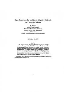
Fig. 1. Performances of csbj augmented with watched data structures on real-world instances.

5.2

Quantifier Watching

In two literal watching in SAT solvers, the two literals allow us to detect when a clause only contains one item, as well as when it is empty. In quantifier watching, we only need to know when the quantifier is empty, and for this, only one watched q-variable is needed per quantifier. The invariants for q-variable watching are: 1. The quantifier is empty and so removed. 2. There is one watched unassigned q-variable in the quantifier. When we remove the watched q-variable, qold , the rules are as follows: 1. Search left and right for an unassigned q-variable, qnew . (a) If qnew exists, watch it. (b) If qnew does not exist, remove the quantifier.

6

Experimental Analysis

We implemented the above ideas in a QBF solver featuring both conflict and solution directed backjumping [6]. In order to test the effectiveness of the watched data structures, we run the 5 different versions of the solver:

Watched Data Structures for QBF Solvers

9

3qbf − 30 vars − 4 lits

1

10

csbj wq 2wl 3wl wcl % True

0

CPU TIME [SEC]

10

−1

10

−2

10

0

5

10

15 20 25 CLAUSES/VARIABLES

30

35

40

Fig. 2. Performance of csbj augmented with watched data structures on random problems with 4 literals per clause

1. 2. 3. 4. 5.

csbj represents the basic solver with the standard data structures, csbj+2wl is csbj plus two literal watching, as described in § 4.1, csbj+3wl is csbj plus three literal watching, as described in § 4.2, csbj+wcl is csbj plus watching clauses, as described in § 5.1, and csbj+wqt is csbj plus watching quantifiers, as described in § 5.2.

All the versions implement the same heuristic. In particular, the literal occurring in most clauses is chosen, and ties are broken by selecting the literal with the smallest index. We considered all of the real world problems available at www.qbflib.org as of 1st May 2003. The problems considered are the Ayari family, the Castellini family, the Letz family and the Rintanen family, giving a total of 322 problems. Of these 322 problems, all the solvers (i) timed out on 93, and (ii) were able to solve 28 in 0 seconds. The results on the remaining 201 problems are shown in Figure 1. In all the figures, on the y-axis there is the time taken by each procedure to solve the number of instances specified on the x-axis. The time out is 7200s. We run the exeriments on a farm of eight identical PCs equipped with a Pentium IV 2.4Ghz processor, and 1024MB of RAM (DDR 333Mhz), running Linux RedHat 7.2(kernel version 2.4.7-10). As it can be seen, neither the two nor the three literal watching structures cause a speed-up in the performances. One reason could be that the average length of clauses on these problems is 3.8. On the positive side, we see that watching clauses provides a significant boost; for example, to solve 167 instances

10

Ian Gent et al. 3qbf − 30 vars − 8 lits − 3 exist

3

10

csbj wq 2wl 3wl wcl % True

2

CPU TIME [SEC]

10

1

10

0

10

−1

10

−2

10

0

5

10

15 20 25 CLAUSES/VARIABLES

30

35

40

Fig. 3. Performance of csbj augmented with watched data structures on random problems with 8 literals per clause

out of the 201 considered, csbj+wcl takes 10s, while the other solvers take 100s. We have considered also instances randomly generated according to model B of [7], with 3 alternations, 30 variables per alternation, 3 existentials per clause, with a total clause length varying between 4 and 12 and a clause to variable ratio from 1 to 40. The results of these experiments can be seen in figures 2, 3 and 4. We see that the clause watching is consistently good in all these graphs. Literal watching does not appear to affect the performance with shorter clauses, but starts to show a good increase in performance as the clause length increases. Watching Quantifiers never shows an increase in performance on these experiments. There appears to be no difference in performance between watching 2 and watching 3 Literals. Indeed, when assigning a watched literal in a clause, in the worst case, both the 3 and the 2 watching literals algorithms have to scan the whole clause. On the other hand, when all but one of the existential literals are negatively assigned, the 3 watching literal algorithm does not need to scan the list of existential literals. This advantage does not produce any significative speed-up on this test set, in which each clause contains only three existential literals. The results for clause watching are not too surprising. It is well known that in QBF the pure literal heuristic plays an important role. Detection of pure literals is difficult however, since we normally need to check every literal in a clause when the clause is removed. Clause watching removes

Watched Data Structures for QBF Solvers

11

3qbf − 30 vars − 12 lits

2

10

csbj wq 2wl 3wl wcl % True 1

CPU TIME [SEC]

10

0

10

−1

10

−2

10

0

5

10

15 20 25 CLAUSES/VARIABLES

30

35

40

Fig. 4. Performance of csbj augmented with watched data structures on random problems with 12 literals per clause

this need. Additionally, most variables have many occurrences in large enough formula, giving rise to large c-literal lists. This means that many clauses will be removed with no work being done. The results for literal watching are what we would expect; with smaller clauses, the watched literal pointers are likely to be chosen with a high probability. As the size of the clauses increases, this probability becomes smaller and so the algorithm operates more efficiently. This is due to the fact that if a literal is not watched, then no work will be done when it is removed. This is similar to the results seen in SAT, where watching literals in larger clauses (i.e. learned clauses) is more effective than watching literals in small clauses. Finally, the results for quantifier watching are also not surprising. In QBF solvers, there is not a lot of work done on the prefix. Additionally, quantifier watching performs the same operations as the standard data structure.

7

Conclusions

We have presented four new watched data structures for QBF solvers. We have implemented and evaluated these implementations on both structured problems and randomly generated problems. The experimental analysis shows that watched data structures do not slow down the solvers significantly. Moreover, watching clauses gives consistently good results on all problems, and watching

12

Ian Gent et al.

both 2 and 3 literals gives better results as the size of the clauses increase, as would be expected from previous results in SAT. Watching quantifiers almost never helps to increase the performance of search in the problems we have observed. Finally, it is well known that in QBF, pure literal detection plays an important role. In SAT, it is a common belief that detecting and assigning pure literals does not pay off. Nevertheless, we think that clause watching could be used to increase the efficiency of pure literal detection, and so prove ultimately that pure literals may be of some importance also in SAT search.

Acknowledgements The work of the authors in Genova is partially supported by MIUR and ASI.

References 1. Davis, M., Putnam, H.: A computing procedure for quantification theory. Journal of the ACM 7 (1960) 201–215 2. Davis, M., Logemann, G., Loveland, D.: A machine program for theorem proving. Journal of the ACM 5 (1962) 3. Zhang, H., Stickel, M.E.: An efficient algorithm for unit propagation. In: Proceedings of the Fourth International Symposium on Artificial Intelligence and Mathematics (AI-MATH’96), Fort Lauderdale (Florida USA) (1996) 4. Moskewicz, M.W., Madigan, C.F., Zhao, Y., Zhang, L., Malik, S.: Chaff: Engineering an Efficient SAT Solver. In: Proc. DAC. (2001) 5. Lynce, I., Marques-Silva, J.: Efficient data structures for fast sat solvers. In: Proceedings of the 5th International Symposium on the Theory and Applications of Satisfiability Testing (SAT’02). (2002) 6. Giunchiglia, E., Narizzano, M., Tacchella, A.: Backjumping for Quantified Boolean Logic Satisfiability. Artificial Intelligence 145 (2003) 99–120 7. Gent, I., Walsh, T.: Beyond NP: the QSAT phase transition. In: Proc. AAAI. (1999) 648–653