Prologue iv. 1. The PER-approach - criteria to rank threats to aquatic ecosystems. 1. 1.1. ... 71. 1.6.2. Marine eutrophication. 73. 1.6.2.1. Effect-load-sensitivity. 79 ii .... Volume. WaleI' exclmoge. Sec:ch1depth. Topograph1cal openness . ⢠- n â¢. - " ..... general index of lake trophy) and oxygen concentration in tbe bottom water.
WATER POLLUTION - methods and criteria to rank, model and remediate chemical threats to aquatic ecosystems
Lars Håkanson and Andreas Bryhn
Part 1. The PER-approach - criteria to rank threats to aquatic ecosystems Part 2. Introduction to aquatic ELS-modeling
Uppsala University Department of Earth Sciences SWEDEN
Printed at Geotryckeriet Uppsala, 2008
Contents Prologue 1. The PER-approach - criteria to rank threats to aquatic ecosystems 1.1. Introduction and aim 1.1.1. Background on chemical threats, especially metals 1.1.2. The PER-concept 1.2. Ecosystem analyses - basic concepts 1.2.1. Defining ecosystem boundaries 1.2.2. Ecosystem indices 1.2.3. Environmental threats 1.2.4. Target ecosystems 1.2.5. Regression models and mass-balance models 1.3. Acidifying substances 1.3.1. Background 1.3.2. The geographical perspective 1.3.3. Acidification and metals 1.3.4. The time perspective 1.3.5. Summary - acidification 1.4. Metals, 1.4.1. Brief background on metals 1.4.1. Mercury 1.4.1.1. Effects variables for mercury in aquatic ecosystems 1.4.1.2. Geographical perspective 1.4.1.3. Effect-load-sensitivity 1.4.1.3.1. Practical use of ELS models in contexts of remediation 1.4.1.4. Time perspective 1.4.1.5. Cause and effect - a chemical theory 1.4.1.6. Remedial measures 1.4.1.7. Summary - mercury 1.4.2. Radiocesium 1.4.2.1. Effect variables 1.4.2.2. Geographical perspective 1.4.2.3. Effect-load-sensitivity 1.4.2.4. Time perspective 1.4.2.5. Summary - radiocesium 1.5. Chlorinated organics 1.5.1. Background 1.5.2. Effect-load-sensitivity 1.5.3. Geographical perspective 1.5.4. Time perspective 1.5.5. Summary - chlorinated organics 1.6. Nutrients 1.6.1. Introduction to eutrophication 1.6.2. Marine eutrophication 1.6.2.1. Effect-load-sensitivity
ii
iv 1 1 6 9 12 12 14 15 16 21 23 23 24 28 30 32 32 32 33 33 34 35 38 42 45 48 50 50 50 54 54 56 58 59 59 62 66 69 71 71 71 73 79
1.6.2.2. The geographical perspective 1.6.2.3. The time scale 1.6.3. Summary - coastal eutrophication 1.6.4. Lake eutrophication 1.6.4.1. Effect-load-sensitivity 1.6.4.2. Area and time perspectives 1.6.4.3. Summary - lake eutrophication 1.7. Conclusions - a ranking of the threats 2. Introduction to aquatic ELS modeling 2.1. Background and aim 2.1.1. The role of prediction 2.1.2. An unambiguous definition of scientific method 2.1.3. Testable predictive models 2.2. Ecosystem sensitivity 2.2.1. Basic hydrodynamic principles and processes for coastal areas 2.2.2. Fundamental sedimentological principles and processes for coastal areas 2.2.3. A coastal sensitivity index (SI) 2.2.4. Lake sensitivity 2.3. Time and area compatibility of data 2.4. Statistical aspects of regression analysis 2.4.1. The ecometric matrix 2.4.2. Confidence intervals and frequency distributions 2.4.3. Prairie's "staircase" 2.4.4. Other statistical concepts and aspects 2.5. Variability and uncertainty 2.5.1. Variability within and among aquatic ecosystems 2.5.2. The sampling formula and uncertainties in empirical data 2.6. Principles determining the predictive success of ecosystem models 2.6.1. The highest possible r2 from Emp1-Emp2; re2 2.6.2. Highest reference r2; rr2 2.6.3. Comparing model predictions with re2 and rr2 2.7. Dynamic and static ecosystem modeling 2.7.1. The classical ELS model - lake eutrophication 2.7.2. ELS modeling of coastal eutrophication 2.8. Model testing 2.8.1. Calibration and validation 2.8.2. Sensitivity tests 2.8.3. Uncertainty tests using Monte Carlo techniques 2.8.4. Uncertainty and sensitivity analysis as tools for structuring ELS models 3. Epilogue Literature references
84 85 85 86 86 90 90 92 95 95 95 95 96 102 102 105 108 110 110 115 115 117 119 119 122 122 124 126 127 131 132 133 133 137 149 149 152 154 161 164 165
Reaching the goal is certainly important for the ride but it is the travelling itself that gives content and pleasure to the stride. (after Karin Boye)
iii
Preface to the edition of 2008 Humans have altered the aquatic environment in a large number of ways, and we regularly get exposed to a multitude of information about various environmental problems via mass media and other sources. These problems vary in terms of severity, geographical spread and duration. Small problems can indeed be solved by individuals, while more complex and widespread problems need large-scale abatement strategies from communities of various sizes and extents. Environmental management concerns the latter type of problems and a basic purpose of environmental management is to direct time and effort towards large environmental problems rather than small and/or imaginary ones. There are two old proverbs that wittingly illustrate which strategies we should avoid if we as professionals really want to achieve something substantial in practice and make a change; one of these proverbs is "not seeing the forest for the trees", and the other one is "straining out gnats while swallowing camels". This book aims at defining methods for pointing out the "camels" among problems in the aquatic environment and at providing tools to prevent, or at least decrease, the swallowing of these camels. To do this, it is crucial to have a system of criteria to structure, analyze and dimension the problems. Subjective approaches are inadequate to the challenges of environmental management. Fully objective scientific methods and results are generally only applicable for specific substances in specific contexts. This book focuses not on the conditions at specific sites but at the ecosystem level, on effect-loadsensitivity (ELS) analysis, on geographical patterns (distribution over area and time), and on practically useful models to aquatic ecosystem management The examples concern the major threats to aquatic ecosystems, such as acidification, eutrophication and contamination and the case studies deal with Swedish lakes and coastal areas. Many of the principles, however, apply to other types of ecosystems, countries or regions. It is often argued that the quality of science is related to the possibility to make meaningful predictions. This argument would give chemistry and physics a pool position in the scientific community and, for example, economics, a low rating. Robert Peters (Peters, 1991) has convincingly shown that many aspects of ecology would belong to the same category as economics, or even theology. But how would predictive ecology rate? This book can be classified as an example of predictive ecology. It has long been argued that due to the complex nature of ecosystems, it will never be possible to predict important target variables, especially not with more comprehensive dynamic models. This book will demonstrate that those arguments are no longer valid. The key lies in the structuring of the predictive models. The aim of this book is to discuss just that and to carry out these discussions within a specific framework where the ultimate aim is to produce meaningful tools for practical water management This book is mainly based on the first two chapters in "Water Pollution" by Lars Håkanson (1999). The second chapter has been revised by Andreas Bryhn and Lars Håkanson in 2008 and now includes examples from Andreas Bryhn's (2008) PhD thesis as well as from "Tools and Criteria for Sustainable
iv
Coastal Ecosystem Management" by Håkanson and Bryhn (2008) - on behalf of some deleted parts of the previous edition of this book. The selection of examples does not mean that the authors disregard the fact that much important related research has been carried out elsewhere by scientists not cited in this book. The point is instead that the case-studies exemplified in this book very well fulfill the purpose of efficient ELS analysis and that data from these examples can be easily distributed by us without permission from other researchers. Some readers may fear that some of the information in this book is out of date, since many references concern conditions as they were during the 1990s. However, the fact is that the roots and extent of virtually all of the mentioned problems have changed very little since then. Eutrophication in the Baltic Sea is persistent. Great advances in combating lake eutrophication were made in the 1970s and 1980s, although much of what remained in the 1990s still remains in 2008 with respect to this problem. Severe and widespread ecosystem effects from lake acidification are still routinely documented although sulphur emissions have drastically decreased. The recovery process from lake acidification is apparently enduring and non-linear. Similarly, high concentrations of some harmful pollutants are still evident in a very large number of lakes and coastal areas despite the fact that much effort has been spent on remediating these problems. The possible exception is radiocesium contamination, a problem which has a low ranking in this book based on information from the 1990s - and the low ranking remains in 2008. The potential ecological risk (PER) value should have decreased somewhat compared to the already low value from 1999, because of the diminishing effects from the Chernobyl accident in 1986, which even at that time were rather limited in the Swedish aquatic environment compared to effects from other problems. Thus, the methodology used in this book, alongside the ecosystem processes, the facts on the ground, and the ranking of chemical threats are still indeed utterly relevant. Part 1 of this book corresponds to 1 week of full-time studies. The focus is on the PER-system, a broad, holistic diagnostic system to structure and rank chemical threats to aquatic ecosystems. A central part of the PER-system concerns effect-load-sensitivity models (ELS), but part 1 does not discuss mathematical and/or statistical aspects of ELS-models. A basic knowledge on aquatic systems may, however, be helpful to understanding the text. Part 2 also corresponds to 1 week of full-time studies. This part concerns the basic elements of ELSmodels, especially dynamic mass-balance models and statistical regression models. Knowledge of basic statistics and mathematics is needed to fully understand this text. The book thus corresponds to 2 weeks of full-time studies.
v
1. The PER-approach - criteria to rank threats to aquatic
ecosystems 1. 1. Introduction and aim A few introductory figures will be used to illustrate the basic approach of the flfst part of this
tex~
the PER-
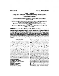
system (Potential Ecological Risk) to structure, analyse and rank chemical threats to aquatic ecosystems. The effect-load-sensitivity analysis (ELS) is an important part of this system. Given a certain threat (load = dose) to a complex ecosystem, crucial questions are: • Which are the target effect variables? and Why? • How can chemical threats to ecosystems be quantitatively ranked? • How is it possible to develop general, validated, predictive ELS-models for the target effect variables based on as few, simple and readily available driving variables as possible? • How can such ELS-models be used as tools to optimise remedial strategies so that the costs for these measures can be quantitatively related to the environmental benefit? • How can such Imowledge be accessible to people responsible for environmental management? All chemical threats cannot be equally important. Subjective criteria to rank are insufficient How is it possible to develop and apply more objective and scientifically warranted criteria to rank chemical threats to aquatic ecosystems? That is the key issue addressed in section 1 of this book. One and the same load of a pollutant may cause very different effects in ecosystems of different sensitivities (= vulnerabilities). In this book, many examples related to the major chemical threats to aquatic ecosystems, such as acidification, eUlTophication and toxic contamination, will be given. Crucial questions are: How are effect, load and sensitivity variables operationally defined? How is the ecosystem defined? The complicated nature of ecosystems makes it very difficult indeed to carry out causal, mechanistic analyses concerning the quantitative linkages between a given threat (like a contamination of nutrients) and variables expressing ecosystem effects. This means that it is very important to define the specific goais and to apply a slTUctured analysis to reach tilOse goals. This is what this book is all about. The problems in complex ecosystems may seem insurmountable, and we will use an initial example to il!uSlTate this. The rest of the book deals with methods to handle such complexities to reach certain defined goals in ranking, predicting and remediating water pollution. Fig. 1.1 exemplifies that tile salinity is a most important abiotic sensitivity factor for the biology in coastal areas. The salinity of the water influences water slTatification, mixing, and hence also the distribution and effects of chemical pollutants. The salinity may also be regarded as a water chemical "cluster" variable in the sense that there are many other water chemical variables that are causally or functionally related to the salinity, like the hardness of the water. Also tile oxygen concenlTation is a most important abiotic variable (see upper right corner of fig. 1.1): The number of species and individuals of the bottom fauna decrease markedly as the load of organic matter increase, and the oxygen concenlTation in tile sediments decrease. So. ulere exist a clear and direct relationship between a "simple" abiotic variable, 02-concenlTation. and lllrget effects. like ule extinction of key functional organisms of Ule bottom fauna.
1
Ecological effect variables
=== ==""'
lem}
Increased contounlnation of organic materta.l.3 Decreased oxygCl COncentration OSlOl:S:l.02S~
SalInJty (%o}
Conductivity Alloilinlty
No
Hardness ......._-------~" Phytoplankton Algae Sallnlty Zoop1a.nk1on
CHEMISTRY
Ca
K
Phosphorus
Fe pH
Fish
BIOLOGY
Peripbyton
Chlorophyll
Oxygen Depth
COASTAL ECOSYS1EM
Bottom fauna
Coastal_
Saiimentation
PHYSICS Volume
Sec:ch1depth Topograph1cal openness
WaleI' exclmoge
1~70_1 ~1B~ I
Water depth (m)
.
--.. "
.•
-
n •
-
3·15_
0-3
"
EroSion
'0 0
...'"os
.
r.lD.!!portatlon: "=un
..
000
•••
so
Exn=ely valuable area
• •• Exn=ely valuable area
Valuable
a=
Iofauna production
Chemical threat. e.g.. from nutrients in coastal areas
(-)
Extremely
v:;?;
tD
valua Ie
~
Fig. 1.1. Illustration of the complex interactions between various chemical, biological and physical factors that may be used to characterize a coasial ecosystem ("Everything depends on everything else"). Example: Top left: The relationship between salinity and number of species. Redrawn from Remane (1934). Top right: The relationship between load of organic malerial, oxic conditions and benthic communities in a marine environment. Redrawn from Pearson and Rosenberg (1976). Lower left: The ETA-diagram (erosion, transportation, accumulation). From Hiikanson and Jansson (1983). Lower ri"ht A model to estimate the fishery biological value of a given coastal area. Redrawn from Hllkanson and Rosenberg (1985). Figure from Hiikanson (1991b).
2
Fig. 1.1 (lower, right) shows that the organic content of the sediment, the sediment type, the water depth and the topographical openness of the coast are linked to the production capacity (the ratio between the production and the biomass). At large water depths (15-70 m) the production of bottom animals is rather low (= 1). At shallow waters the production can be very high, especially in semi-enclosed bays with mixed sediments and in estuaries. This depends on the type of the sediments, Ille habitat for Ille bottom fauna And the sediment type depends largely on the relationship between the effective fetch and the water depth (see fig. 1.1, lower left diagram). The effective fetch is a measure of the free open water surface over which the winds may act upon the waves; the larger the effective fetch, the higher the waves, the larger the wave energy and Ille greater the capacity of the waves to erode and transport the material on the bottom. It is evident that most of the variables illustrated in fig. 1.1 are more or less related to each other in an extremely complex web of relationships. To establish such relationships quantitatively, it is essential to use a rational and structured analysis, and this is what the following section would like to convey. Another motive for this book is to highlight problems concerning causal analyses, i.e., the problem in science to differentiate between cause and effect. Fig. 1.2 offers an example of this concerning an important issue in water management: Effects of land-use, in Ibis case extensive lumbering, on water quality, in this case lake water
colour. It is evident Illat many activities in the catchment area influence the runoff of substances from land to water, e.g., coloured substances, like humic materials, metals and nutrients. The aim here is neilller to discuss this problem nor to exatrtine the processes regulating the transport of water, ions, substances and materials from the catchment, into rivers and lakes. The aim is simply to give one example of tlle importance of understanding the concept of cause and effect, and the need for validated predictive models. Fig. 1.2A illustrates the month-to-month variation in lake colour in lake 2106, Stora Kr6ntjfun. Because the catchment area of ulis lake was extensively lumbered during late 1986 and early 1987, it is tempting to conclude Ulat ulOse extensive and easily identifiable operations caused the drastic increase in lake colour observed in fall 1986. That surmise would, however, be more wrong than right. Fig. 1.2B demonstrates that more or less exactly Ule same seasonal pattern in lake colour could be seen in another lake, lake 2105, Hoimsj6n. There were no timber operations at all in that catchment area during these years. The increased values of lake colour during fall, and the general pattern in lake 2105 during 1986, is not linked primarily to forestry but to regional climate and hydrology. It is likely Illat tree-harvesting increases the transport of coloured substances to lakes. But it is also a fact Illat such increases cannot be clearly distinguished from other factors in this case. Fig. I.2C shows that lake colour fluctuated markedly among different years (1986 to 1989) in lake 2106 depending on fluctuations in
precipitation, temperature. etc. The lesson from this example is that verbal "causal explanations" for certain phenomenon are temptingly easy when only one or few factors (= facts) are known. In fact, causal explanations of ecosystem level phenomena are very difficult. The concentrations of a given chemical variable (e.g., lake colour) or the amount of some biological variable are so frequenUy multiply determined that we should suspect facile explanations. The answer to this scientific question depends in ecosystem contexts very much on the scale in focus and On Ule availability of quantitative models which include all the key processes. Had such a model been available, it would be possible to conduct simulations to see if it is realistic to surmise !bat the land-use operation in this example is likely to be responsible for Ule increase in lake colour and nOl, e.g., increased runoff from heavy precipitation.
3
Lake 2106. Stofa Krontjiirn
A ........ 180
'a.S-
r--
Lumbering
160
'00 140
.§.
120 100 80 60 u 40 .I: n1 20 ....l
S o ao
---------~'"
~,
~--
2
3
4
5
199&
~ Effect oflumbenng?
6
7
8
9
10
II
12
Month
5a.
200
.§.
160 140 120
J-
100
'00
5
'8
"
.I:
j
B.
180t-_-~"
80 60 40 20
Lake 2105. Holmsjon ---1986
No cutting or ditching
0+--+--+--+--+--+--+--r--+-~__~4
2
3
4
5
6
7
8
9
10
II
12
Month ......... 180
'Sa.
'00
.§.
5
o '0o
"
.I:
'"
....l
160
---1986
140 120
-----1987
100
80 60 40 20
------1989
2
3
4
5
6
7
8
9
10
II
12
Month Fig. 1.2 A. Seasonal variability in lake colour (based on monthly data) in lake 2106 during 1986. Extensive cutting operations were carried out in this catchment area during fall 1986 and early 1987. B. Seasonal variability in lake colour (based on monthly data) in lake 2105 in 1986. No cutting operations were carried out in this catchment area.
C. Seasonal variability in lake colour (based on monthly data) in lake. 2106, over four years, 1986 to 1989. Based on Hilkanson and Peters (1995). There are at least three different approaches based on three different scales to !be issues discussed in this book: 1. The mesocosm-scale concerns artificial but realistic micro worlds (see fig. 1.3). 2. The ecosystem-scale concerns real, natural ecosystems of a given extent in area (0.01 10 1000 km 2 ) and time (days to years).
3. The multi-media-scale including water, biota, sediments, aunosphere, i.e., large geographical areas or long periods of time (Mackay, 1979; Mackay and Paterson, 1982). The focus of this work is at the ecosystem scale, and not at other smaller or larger scales.
4
V ft
r.!........... .·.......... :.:.: ........... ~ . .............
c
,
· .......... . .. ......... ... ... ·....... .......... ........ ... .. ...........
........... .·............ ........... . . . . . . . . . .... ........... ........... . . . ..... . . . ., ....... . . . . . ...
A
=Reservoi r
B = Si phon
C = Ges trep
Fig. 1.3. An example of a mesocosm. A model of the shallow-water ecosystem of the Baltic in an outdoor basin (8 m 3). The most sensitive key functional organisms for a given chemical contamination are the target organisms. The concentrations that cause effecLS on the target organisms are the critical concentrations. From Hiikanson (1990a). Table 1.1. Various chemical ulreaLS and some examples of ecological effecLS. There are also many physical threaLS to aquatic ecosystems, like the building of dams, piers and marinas, and many biological threats, sucb as the intrnduction of new species. Chemical threat
Ecological effects
1. Acidification
Increase in fUamentous algae Reduced reproduction of crustaceans, snails, bivalves and roach
2. Eutrophication
Decrease in Secchi depth Increase in cbloroJlhyll-a and Hypolimnetic oxygen demand'
3. Contamination 3.1. Metals
Increased concentration in fish for human consumption
3.2. Radionuclides 3 '1 Qroanic toxins
Decrease in reproduction of key organisms, e.g .. zooplankton, benthos and fish
The effect variable is a key concept in this approach. It is of vital importance that tile reader realises what is meant and not meant by the effect variable. The effect variable can be identified by mesocosm studies and then applied in the real world, the ecosystem. A mesocosm is a reproduction of the real ecosystem (e.g., a given lake type) that is as close to reality as possible in a reasonably large "laboratory scale" (Landner, 1989; Lehtinen et al .. 1996, 1998). The mesocosm should contain tile fundamental functional groups which form and characterize the actual ecosystem. In this connection, the purpose of the mesocosm is to study, under controlled conditions, the substance of interest in order to see (1) which parts of the ecosystem are first damaged and (2) the concentrations at which the damage occurs. Naturally, it is not possible to simulate in a mesocosm everytiling tim bappens in nature, such as the influence of weather, wind, currents and other animal species than those included in the mesocosm. However, it is important that tile mesocosm studies lead to identifying target effect
variables and critical concentrations because this is essential for studies in real, natural ecosystems, the target scale in practical water management and in tilis book.
5
So, tbis book focuses on tile ecosystem-scale, and on tbe major chemical threats to aquatic ecosystems (table
l.l): 1. Acidification,
2. Eutrophication, and
3, Contamination (of metals, organic toxins and radionuclides). • In acidification research, tbe target effect variables could be measures of reproduction damage to the most sensitive fish species (like roach), and target operational variables could be natural or preindustrial average values of lake pH and/or alkalinity. This information is important in remedial liming because there is no benefit to raising pH above tbe natural level and because excessive liming increases cost needlessly. The economics of liming are a major concern in Sweden where the costs for lake liming to control the effects of antbropogenic acidification now exceed 150 million Swedish SKR (about 20 -25 million U.S. dollars) per year. In tbe U.S.A .. tbe narurallevel was a target variable, because of the intense debate about whetber cultural acidification had even occurred. • In eutrophication, likely target variables are mean, representative ecosystem values of chlorophyll-a (a practical, operational measure of algal biomass and an indicator of primary productivity), or Secchi depth (as a general index of lake trophy) and oxygen concentration in tbe bottom water. The concentration of phosphorus in lakes can be used to predict all tbese target variables for lake eutrophication. • In Ecotoxicology, tbe target variables might include mean ecosystem concentrations of toxic substances in fish destined for human consumption (such concentrations are often used to set guidelines, blacklisting limits and environmental goals) and operationally defined, ecological effects on key organisms, like mortality, reproduction and abundance of important functional groups in defined ecosystems. • In Radioecology, tbe goal may be to measure and predict tbe concentrations or activities of radionuclides in (1) water used for irrigation and (2) in fISh for human consumption. The emphasis is not prediction for specific instances or samples (e.g., for Fish B from location A at time X) but ratber to get a good quantitative picrure for larger areas over longer periods of time, Le., for entire ecosystems.
1.1.1. Background on chemical threats, especially metals This book will use mercury and radiocesium as type elements and lakes and coastal areas as type ecosystems to illustrate many of the fundamental principles and processes regulating tbe spread, biouptake and ecosystem effeclS of contaminates in general. Mercury belongs to a group of elements often referred to as heavy metals (Le., metals with a density> 5/cm 3). These metals generally form oxides and sulphides which are often very hard to dissolve, and Illey tend to be bound in stable complexes witb organic and inorganic particles, Ille "carrier particles". TIle great interest in heavy metals in aquatic ecotoxicology derives from the fact that some of Illese elements are supplied to water systems in great excess by man, and tilat some of them are hazardous to the aquatic life because (see Bowen, 1966; Forstner and Muller, 1974; Forsmer and Witunann, 1979; Salomons and F6rsmer, 1984): • Tbey can disturb enzymatic systems because of the high electro-negative affinity for reactive groups on ille enzymes, like amino or sulfhydryl groups. • They can form stable complexes with essential metabolites. • They can catalyse ille breakdown of such metabolites. • They can permeate the membranes of cell. • Metals can also substitute oiller elements wiill important functions in Ille cell metabolism.
6
Table 1.2. Tbe abundance of various elemenlS (in ppm) in igneous rocks, soils, fresh water, land planlS and land animals (from Bowen, 1966). Igneous rocks Ag Al As Cd Co Cr Cu Fe Hg Mn Mo
Ni Pb Sn
V Zn
om 82,000 1.8 0.2 25 100 55 56,300 0.08 950 1.5 75 12.5 2.0 135 70
Soils 0.1 71,000 6.0 .0.06 8.0 100 20 38,000 0.03-0.8 850 2.0 40 10 10 100 50
Fresh water 0.00013 0.24 0.004 0; if At = 0, tilen this is not a coastal area but a lake near the sea). For such areas, a significant portion of the materials suspended in the water can "escape" from the coastal area to the open water area or to surrounding coastal areas. This is not the case in the same way for lakes. So, coastal areas with small mean depths will generally bave coarse bottom sediments with small amounts of fine materials of organic and inorganic origin causing high water turbidity when resuspended. It is always important to define the presuppositions of any model. When and where will it apply? The definition of the ecosystem boundaries is one crucial aspect of this for ELS-models for coastal areas.
1.2.2. Ecosystem indices In environmental management it is important not to use personal viewpoints as criteria to rank threats as a basis for action, but to have a more objective approach. There is a growing awareness that much better individual "indicators" and aggregated "indices" of environmental health are necessary because they alone could provide a rational structure for decision-making in the environmental sciences (Bromberg, 1990; OECD, 1991). An index (an aggregated measure) is generally distinguished from an indicator (a single variable), and an ecosystem (a single instance, like a lake or a field) from an ecosystem type (the summation of several to many ecosystems). This book discusses two different types of environmental indices: PER, in section I, and LEI (the Lake Ecosystem Index), in section 4. PER is a general, holistic index Calculated from the geographical extent and duration of a defined effects variable (E or Ecrit). LEI is calculated from changes in biomasses of key functional organisms related to chentical remedies, which can alter these biomasses relative to defined natural (= reference) conditions. These two systems will, hopefully, be a step
to~vard
a more objective platform for dimensioning environmental
problems. Certainly, the complexities involved in establishing simple, practical and meaningful ecological indices or effect variables sometimes seem insurmountable. Still, the benefits of even crude indices like PER are so great that they are well worth pursuing. So long as one can clearly state ones criteria, theories and evidence in these complicated matters, then these components can be discussed, tested and improved. A frame of reference is required to assess the status of the environment. Since 1987, many countries have accepted "sustainable development" as a goal for environmental and econontic policy. The term was introduced in the final report of the Commission for Environment and Development (the Brundtland Commission). However, this phrase is empty unless it is defined in terms of operationally measurable properties, desired goals and relevant data. There are alternatives to choosing ecosystem as the basis for environmental typology (Mackay and Paterson, 1982; O'Neill et al .. 1982; Cairns and Pratt, 1987). Instead, one might use different geographic areas or different media such as air, water and soil. There is, however, a clear international trend towards consideration of tile "healtil" of the different ecosystems (Bailey et al., 1985).
14
1.2.3. Environmental threats Tbe environmental threats to life on this planet include: Chemicals involved I.
2.
Climate change Reduction of the ozone layer
3. 4.
Acidification Air pollution
5.
Eutrophication Contamination of metals & radionuclides Contamination of organic toxins Health effects and inconveniences Changes to the rural landscape areas worthy of protection Reduced biological diversity Introduction of exotic and new organisms Over-exploitation of natural resources
6.
7. 8. 9. 10.
II. 12.
C02, etc. 02, freons, etc. S,N
S, NOx, Pb, etc. P, N, etc. Metals and radionuclides DDTs, PCDs, dioxins, etc. CO, Pb, S, etc. Xenobiotics Xenobiotics
Ten of these twelve threats involve chemicals. A set of ecological effect variables is expected to reflect such threats and the extent to which they affect the ecosystem. Note the difference between biological effects for individual animals or organs and ecological effects for entire ecosystems. Practically useful, operational effect variables should be: measurable, preferably simply and inexpensively clearly interpretable and predictable by validated quantitative models internationally applicable relevant for the given environmental threat representative for the given ecosystem. The effect variables or indices must be chosen so that the "distance" between the present environmental status and an identified environmental goal can be determined. Ideally, environmental effect variables should be comprehensible without expert knowledge. In fact, one reason to develop such measures is so that politicians and the general public can understand the present condition and future changes in the environmenL The creation of an ecosystem index like PER requires aggregation of information. For example, if the indices for all ecosystems in a region are averaged, this figure is then a regional ecosystem index. A still higher level of
aggregation is obtained if one sums (or averages) the regional indices for each ecosystem type (for lakes, forests, agriculruralland, etc.) into a single regional or national environmental state index. An aggregated index of environmental health would complement the picture of the country's economic development given by the GNP (gross national product). An environmental state index of this kind could be compared with a consumer price index; environmental indicators would correspond to different items, the national environmental index for a given ecosystem type would be similar to the value of a class of goods. Ecosystem indices would have the advantage of expressing the environmental status simply, but they simultaneously pose problems in that a great deal of valuable information is lost in aggregating the individual measures. This disadvantage is reduced if one knows exactly what an index represents, and if one can access these
15
individual components as required. Ideally, Ibe same basic framework would be used at bOlh Ule national and regional scales. However, since problems and priorities cannot be completely congruent at different levels, Ibe framework may be adapted to Ibe different requirements of different levels. Tbe national level may address largescale Ibreats, perbaps originating outside Ibe country, like acidification of soil and water, whereas Ibe region can address more local problems, like Ibe eutrophication of lakes. A crucial question is: How could Ibis be achieved in practice? The following parts of Ibis book will give one avenue to this very difficult goal.
1.2.4. Target ecosystems An environmental index must be based on Ibe status of some crucial characteristics of chosen ecosystem types, sucb as: 1. Forests
2, Agricultural land 3. Natural land 4. Freshwater
5. Coastal areas and 6. Urban areas.
These are the six basic ecosystem types. As pointed out, it is extremely difficult to distinguish cause and effect in natural ecosystems. One cannot base Ibe PER-number or the ELS-model on a full understanding of Ule ecosystem. In complex ecosystems "understanding" at one scale (e.g., Ule ecosystem scale) is generally related to processes and mechanisms at Ibe next lower scale (e.g., the scale of individual animals andIor plants), and the-explanation of phenomena at this scale is related lO processes and mecbartisms at the next lower scale (e.g., the scale of the organ), and so on down to the level of the alOm and beyond. In environmental management, the predictive ecologist must often find a balance between answering interesting, often important, questions of understanding, and delivering a practical tool to society. If an ecosystem index were based on a causal analysis of what takes place at the cellular level, then at levels involving organs, individuals, populations, and finally at the ecosystem level, one would wait an eternity before the index could be developed. For the foreseeable future, ecosystem indices like PER are more likely lO be based an practical considerations of predictive power and sampling ease, rather than full causal priority. What, then, does the strategy look like if one wants to develop an ecosystem index like PER in practice" The ftrst problem is that each ecosystem type, e.g., fresh waters, is not a single entity. It consists of many sub-ecosystems (fig. 1.7). A general resolution about the base of this approach is probably impossible, but questions about Ule appropriate hierarcbicallevel of analysis are relevant to specific Ulfeats. Fig. 1.7 lists Ibe 12 general environmental Ulfeats mentioned earlier. If one starts with the threat to fresh waters, it is clear that contamination of, e.g., metals/radionuclides Ibreaten fresb waters and that these Ibreats might be manifested in, e.g., reduced biological diversity and contaminated fish. It is also clear that some of these 12111rcats are not relevant to fresh waters. "EveryUling does NOT Ibreat everything elsc"!
16
Ecosystem
Fresh water
Soil water
In-flowareas
Surface water
Lakes
l0ut-flowareas\
Target ecosystem for metal contamination
Mesotrophic
t tt ~
"» ~ "c: S 0
u '1:
.
"t: .c "u .!l
.5"
"0. '" 0 s 01
.c
~
0
.S""
" c
0
~
1
2
t t t t t t t t
u .g" '" '"
~
'0
c:
0 '"0. s 0
'0
'"
.~
0;
'"
4
t
'c
.S! .c
S
"'"
"
u
"g
.!< '0
.0
0
'c
g.
] -
%
0 ~
5.4
Sulphur and nJtrogen
Ix
0.:35
B 0.30-0.35 [j
0.25-0.30
('{ Q
0.20-0.25
V0
o
=--·"'II",!I""'II."'i!i"'=-1 j
O~~~~~~~~~~~~~~LJ
U. n=26
100 90..E·
WLL n=23
~
DAL n=4
Se
n=7
IF
n=B
(n=ll)
Lake liming
1 SD Error
'
80j----------------------------1
80 g), small perch « 12 g) and pike when fallout is 50 kBq/m2 , theoretical water retention time I year and water conductivity 4 mS/m. Lower: The same for char and brown trout in Swedish mountain lakes. From Hakanson et al. (1992). model predicts the initial empirical concentrations rather well the "tail" of the curve is not realistic. This motivates wby aboutIO years should be added to the time scales given in fig_ 1.39. The model calculations given in this figure indicate, e.g., that in year 2010, the Cspi-values will. on average, be in the range 100-300 Bq/kg ww within the most exposed areas in Sweden. The maximum Cs-concentrations in pike in this year should be below 1500 Bq/kg ww. In the year 2020, almost all lakes should have Cspi-values lower than 20 Bq/kg ww. From recovery models andlor from empirical time-series of dala, one can determine values for the ecological halflives for cesium in fish after the Chernobyl event. Tbe ecological balflife reflects the actual decrease in contaminant concentration for fish in real ecosystems, while the biological halflife reflects the decrease in individual fish if they are place in uncontaminatedenvironrnents and the decrease is regulated by melabolic activities. The new dynamic model (section 3.1) gives an initial ecological halflife, from month 30 when the peak value of 28,000 Bq/kg ww is attained to month 70 when half that value is attained, of about 40 months for pike in the Finnish lake, Iso Valkjarvi, which has a long theoretical water retention time of 3 years (fig. 1.40). Note that this initial ecological halflife has been determined relative to the year when the maximal Cs-concentration
57
2000
2010
1990
2000
2020 2010
Cs·137 tn pike
(Bq/kg ww)
Cs·137 in pllte (Bq/kg ww)
~ :lOO~OOO
ri
o
1$'JO~3000
IB
:100·1$00
Q
0< 300
Cs·137 In pIke (Bq/kg ww)
101)-300 60-100
o
'~20
0«
090
2-10
>10 6-10
30-40
10-15
4-6
40-60
AO
>15
25 em) .. Coastal areas outside the range afthe model parameterS
Fig. 1.59. An ELS-model for coastal eutrophication where tbe concentration of chlorophyll-a is used as an operational effect variable and tbe concentration of total-N (TN) as a load or response variable. The model is also discussed in section 2. 2. 02Sat depends on botb load factors (table 1.8 gives a list of all such factors) and sensitivity factors linked to the size and form (the morphometry) of tbe coast. "The way tbe coast looks regulates how the coast functions". It should be noted that the mean 02Sat-value is NOT a constant. but a variable, and that a model based only on
morphomeuic parameters can NOT be used for site-specific predictions of time-dependent y-variables. The empirical model presented in fig. 1.60 is based on nuuient concentrations (total-N and total-P; load or rather response variables) and morphometry to predict long-time summer averages of 02Sat for entire and well-defined coastal areas.
One very important question concerns the definition of the coastal ecosystem, i.e., where to place the boundaries toward the sea andlor adjacent coastal areas. It is crucial to use a technique thal provides an ecologically meaningful and practically useful defmilion of the coastal ecosys!em. The coastal boundaries are, in tilis context, operationally defined by means of tbe "topographical bottle-neck !echnique" calculated from the exposure (or the openness toward the sea and adjacent coastal areas), see fig. 1.6.
80
Table 1.8. Variables for eutrophication effect and load (concentrations are expressed as mean values for JuneSeptember and load variables as mean values for 2 years), morphometric parameters and Statistics for 23 Baltic coastal areas. From Hiikanson (1994). Symbol
Variable
Units
Mean
Min.
Max.
m mg om-3 gom-2o day-1
3.6
1.0
6.9
2.76
0.90
9.60
7.53
1.07
17.56
gom-2odal" 1 mgol- 1
25.85 7.06
5.31 1.05
82.53 10.00
%
67.0
8.5
98.1
m0o -m-3 m0oe m- 3 m0oe m- 3 mg om- 3
335
256
417
27
14
52
23
14
31
4
2
12
14,979
3656
81,501
Eutrophication effects Secc
Secchi depth
Chi
near-surface chlorophyll-a
SedS
near-surface sedimentation
SedB 02B
near-boltom sedimentation
02Sat
near-bottom 02 saturation
near~boltom
oxygen conc.
Nutrient concentration
TN
near-surface total-N
near-surface inorganic-N TP near-surface total-P near-surface inorganic-P IP Nutrient load IN
Ntot
total N load
ANtot
total N load (area-weighted)
kg Noy-1 kg N okm- 2oy-1
4023
1532
19,585
PtOt
total P load
kg poy-1
1472
total-P load (area-weighted)
kg N okm- 2o y-1
492
93 27
6956
APtOt
3177
Size parameters
Dmax
maximum depUl
m
22.6
11.1
46.9
a
water surface area bottom area section area towards the sea water volume
km 2
4.71
1.05
14.15
km 2
4.49
0.92
13.90
km 2
0.014
0.001
0.082
km 3
0.033
0.006
0.18
Ab At V
Form parameters
Dm
mean depUl = Via
m
7.6
3.8
13.8
xm
mean slope
%
4.83
2.21
8.17
Dr
relative depUl = Dmax o,Jrr/20 o,Ja
%
1.12
0.46
2.68
F
shore irregularity form factOr = 30DmlDmax
190.5
104.2
507.4
1.05
0.57
1.47
Yd
%
Special parameters
E
exposure = 1000AtiAb
0.39
0.045
1.27
Ff
filter factor
km 3
6.73
0.059
30.71
MFf
mean filter factor
km 3
1.32
0.012
6.49
BA
proportion of A-areas
%
19.5
80.9
BET
QroQortion of ET-areas
%
80.5
0 19.1
81
100
&t
For mean depth 100
= 7.6 m. filter factor = 6.7 km3 and volume = 0.33 km3
"0 0
1: 90 n>
0-
-ci 0
SENSITIVITY VARIABLE Theor. deep water ret. time (Td In deys)
80
'-
0-
-" n>
'"CO ..J
.c 70 C>
50
'">D
~
\0
0
~ ~
0 0
~
RESPONSE FUNCTION (TN + 100TP) (mg/m3)
Step Step Step Step Step
1: Nutrient response function (TN+10"TP) 2: Theor. deep water retention time (Td) 3: Mean depth (Om) 4: Fitter factor (Ff) 5: Coastal volume (V)
r2-value 0.49 0.76 0.89 0.91 0.93
Data from 23 Baltic coastal areas Model: 02Sat= 1OO~SIN{ 14.827 -4 ,4648.~LOG(TN+ 1 O~T P)-O.403 "LOG{ 1 + Td)-1 ,04S"LOG(Dm)-O,021 ~FI+O,275·LOG(V))
Fig. 1.60. An ELS-model using the oxygen saturation in deep water, 02Sat, as opemtional effect variable for Baltic coastal areas; critical concentration, "ladder" and model (see section 2 for model derivation). The results shown in fig. 1.60 give 02Sat versus a load function plus sensitivity parameters. One can note that 02Sat may be predicted quite well from the load function (1N+ I O*TP) plus four morphometric (sensitivity) parameters: The higher tile load of both N and p. the lower 02Sat; the longer the theoretical deep water retention time (Td), the more sheltered the coast is (given by the filter factor, Ff; see fig. 1.63 for definition), the deeper and larger tile coastal area and the lower the filter factor, the lower 02B. The r2-value after five steps is 0.93. The most powerful predictor is the nutrient function. Note that in models of this kind one can often replace the model variables (tlle x-variables) with related variables from the same cluster or functional group, e.g., Ff may be replaced by tile section area; the load function (1N+lO*TP) could be replaced by other types of load functions. Since "everything is related to everything else" in ecosystems like these, it is generally difficult or impossible to give clear-cut causal explanations why a certain xvariable is linked to a certain y-variable. Models should be built upon simple, easily accessible, logical variables which show a minimum of inter-dependence.
82
Manne eutrophication Nutrients
(phosphorus and
r::-::71
Areas with low
~
Areas with
oxygen
~ concentrations «
nitrogen)
2 mgJU
lam1nated sedIments
and no bottom fauna
Finland Sweden
o
2 3 (em)
Increased ccntamlnation of organic materials Decreased oxygen concentration Polen
Germany Fig. 1.61. Illustration of the areal distribution of the eutrophication problem in marine areas surrounding Sweden (based on Ambia, 1990); on the west coast, low 02-concentrations occasionally appear in bottom water; on the east coast, laminated sediments occur over vast areas; and an illustration of ecological effeclS on bottom fauna from increased organic load (oxygen consumption) in sedimenlS (based on Pearson and Rosenberg, 1976). From Hakanson (1994). The model in fig. 1.60 should NOT be used for other types of coaslS. It cannot, e.g., be used for coastal areas dominated by heavy tides. Many factors could potentially influence 02Sat, the effect variable in this case. It is easy 10 speculate and qualitatively discuss such relationships. With empirical data it is possible to quantitatively rank such factors and derive predictive models based on just a few, but the most important, faclOrs influencing 02Sat (for coasts of !be given type). The given model could (statistically) explain 93% of the variability in the given y-variable among !be 23 coastal areas. A "naturai" 02Sat could be estimated from the model, if it is possible to estimate "natural" (or reference) background values of TN and TP. If the actual 02Sat-value of the coast differ from such a "natural" value, then !bose divergences may be discussed in a quantitative manner.
83
Fig. 1.62. Extension of laminated surficial sediments in the Baltic Proper. Modified from Jonsson (1992). 1.6.2.2. The geographical perspective Fig. 1.61 illustrates why marine eutropbication is sucb a problem: Very large areas along the Swedish west coast bave bottom areas where the concentration of oxygen occasionally decreases below the critical limit (Eerit) of 2 mg/l, or 02Sat = 20%. A less scbematic map based on empirical measuremeDiS is given in fig. 1.62. Many benthic animals die if the 02-concentration is lower than 2 mg/l (fig. 1.61 rigbt), bioturbation is halted, and laminated sediments appear. The figure also sbows that very large areas in the Baltic Proper bave laminated sediments. Recent studies (Per Jonsson, pers. comm.) bave also demonstrated that laminated sediments appear over larger and larger areas also within the coastal zone. Tbis is alarming since the coastal zone is regarded (see Hakanson and Rosenberg, 1985) as a "nursery and pantry" for the open water areas. Tbe eutropbication conditions in the open water areas of the Baltic are governed by the tributary nutrient fluxes to the Baltic, and by the bydrodynamic conditions, such as the coastal currents and the water exchange. The conditions in the coastal zone are dynamic and strongly influenced by the conditions in the open water areas (a typical water tlllUover time for a coastal area is 2-4 days). Also sbeltered bays deep within archipelago areas are strongly influence by the bydro 0. C 0.-
-0
:I:
$
m
"
:I:
"E n; g
"
c: 0 c
*
a:
C>
c:
C 3:
[
~
w
~
al
"
c: :;
a:
c:
c:
n;
;;;
:E
Ern
.2 0
0.
e '5
UJ
0
c: .!!!
c:
"'0
E
c: -U 0
0 0 0
X
....0
~
"
13 8. w
g"
E
Fig. 1.68. Different causes for the reduction andlor extinction of fISh communities in Swedish lakes. Note that acidification in most important among these causes, but that also eutrophication has implied significant changes in the structure of fish communities and that many other causes than chemical threats, like hydropower constructions, ruined spawning areas and introduction of alien species, have changed the fish communities. From EPA (1997). spill, and that such accidents may be treated separately or taken together in the PER-analysis. This is a matter of definition of the presuppositions. In table 1.10, the evaluation concerns just this particular accident. The PERnumber for this case-study is 56 (E
=7, A =2 and T =4).
The results in table 1.10 are open to debate and improvements!
93
..,.
\0
56
PER= E*A*T 700 240 72 216 300 560
-PER ranking priority for action I 4 6 5 3 2
Areal distribution: Duration In time: l=no ecosystems widl E = 10 and/or E = Eerit 1= no effects 2=a few ecosystems with E = 1O!Ecrit «25 lakes or coastal areas) 2= effects (E = 10/Ecrit) for less dlan 1 month 3= more Ulan 1 month 3=several ecosystems widl E = 10/Ecrit (25-100 lakes) 4= more than 1 year 4=many ecosystems with E = 1O!Ecrit (100-400) 5= more than 10 years 5=most ecosystems in a region with E = lO!Ecrit 6;;;:ccosystems in many regions wilh E;::; 10/Ecrit 6;::; more than 20 years 7=more than 25% of Swedish lakes or coastal areas with E = IO/Ecrit 7= more Umn 40 years 8=more than 50% of Swedish lakes or coastal areas widl E = IO/Ecrit 8= more than 80 years 9=more than 75% of Swedish lakes or coastal areas widl E = 10 9= more than 160 years IO=alllakes or coastal areas in Sweden wiUl E = lO/Ecrit 10= effects (E = 10/Ecrit) for mOre than 320 years
4
10 10 6 6 5 7
(T)
Duration iii Ume
/
Note 1. For mercury contamination widl E = 3, the A- ,md T-values arc determined for the guideline limit for the target variable, Hgpi = Ecrit = 0.5 mg Hg/kg ww. Note 2. For radiocesium with E = 2, Ule A- and T-values arc determined for the guideline limit for the target variable, cesium in fish for human consumption, Ecrit =1500 Bq/kg ww. Note 3. For organic contamination with E = 6, A and T are determined for the "critical" limit related to EOCI-concentrations in surface sediments of 500 ~g EOCI/g org. material. Note 4. As a comparison to the cases treated here, data are also given related to the Tesis oil spill (from Kineman et aI., 1980).
Effect variable: 1=00 known or likely ecosystems effects 2=unlikely ecosystems effects using statistical methods 3=likely but low ecosystems effects using statistical methods 4=probable ecosystems effects using statistical medlOds 5=small real ecosystems effects 6;;;:clear real ccosystcms effects 7=substantial real ecosystems effects 8=large real ecosystems effects 9=very large real ecosystems effects 10=lOtal collapse of real ecosystems
2
7
Marine/coastal
Tsesis oil spill
6
8 6 6 8
10 3
Lake Lake Lake Marine/coastal Lake Marine/coastal
Acidification Mercury contamination Rndiocesi urn comamination Organic toxin contamination Eutrophication, phosphorus Eutrophication, phosphorus and nitrogen 2 6 10 10
Erfeet vadabl' (E)
Ecosystem
Swedish 3guatic ecos;),stems Threat Areal distribution (A) 7
Table 1.10. A compilation of PER-criteria to rank the chemical threats to Swedish aquatic ecosystems
discussed in this work.
2. Introduction to aquatic ELS modeling 2.1. Background and aim Aquatic ecosystems are very complex webs of physical, chemical and biological interactions (fig. 1.1). It is generally both costly and laborious to describe their characteristics, and to predict them is even harder. To develop scientific programs of conservation, management and remediation is an even greater challenge. Every aquatic ecosystem is unique, and yet it is impossible to study each system in the detail necessary for case-by-case assessment of ecological threats, and proposals for remedial measures. In this situation, quantitative ELS models are essential for predicting, making environmental assessments and directing intervention strategies. 2.1.1. The role of prediction There are two important reasons to spend time and effort at quantifying important environmental features and processes. Formulating quantitative descriptions aims at representing aquatic ecosystems the way they appear, and as closely to the "truth" as possible. Quantitative prediction is necessary for testing assumed scientific relationships; whether a change in one ecosystem variable may affect another variable. Thus, predictions obviously have great importance for environmental management. Environmental managers, policymakers, and the general public often have a considerable interest in knowing what the probable environmental effect will be of a certain policy or measure, such as liming or building sewage treatment plants. The ability to predict important goal variables, such as pH, the Secchi depth or the algal bloom intensity (as measured by Chl) in aquatic systems is thus very useful in practice as a communication tool between natural scientists and the rest of the world. Furthermore, high predictive power is an important scientific goal in itself. The certainty with which we can predict changes in water quality from changes in external factors, such as nutrient loadings, is a direct, quantitative indicator of how well we understand scientific relationships (Peters, 1991). This certainty is commonly referred to as the predictive power, or the forecasting power. An alternative approach to predictive models is the use of conceptual models, which is still attractive among some environmental analysts. A conceptual model can be a scheme over important features in an ecosystem, such as fish, nutrient concentrations, etc., with arrows indicating the causal paths in the ecosystem; i. e., to indicate how one ecosystem feature is influenced by others. However, a conceptual model does not convey any quantitative information about what happens to the ecosystem if external factors (climate, pollutants, large-scale fishing, etc.) change compared to present conditions. Thus, the complete structure of a conceptual model is often difficult to test against empirical data, because there is no direct connection between a conceptual model and empirical indicators. Instead, its credibility can to some extent be established indirectly (indirectly tested) by empirically testing measurable theories derived from the model. However, within the field of lake restoration, the success record of conceptual models has been relatively meager (Peters, 1991). Conversely, quantitative, predictive methods have thus far been instrumental in massive and successful programs of eutrophication and acidification control in many lakes around the world. Thus, ELSanalysis of aquatic systems relies on predictive modeling because of its greater scientific potential. 2.1.2. An unambiguous definition of scientific method If one agrees that science has a unique and important role in society, and that it is not a complete waste of resources to spend large sums of governmental and private money on scientific research, then this insight should lead one to conclude that the unique status of science requires that it be defined in an
95
unambiguous manner. There are many variants available in the philosophy of science which in one way or another defines science as "something that scientists do" (Peters, 1991). According to such definitions, we would be able to consider astrology, alchemy and various holy scripts as science, since many scientists have been involved in those fields during history. However, if we admit that these fields have generated very limited scientific success and predictive power over the years compared to the primary parts of, e. g., physics, medicine and ecology, then we apparently need a different definition of science. To this date, Karl Popper's (1902-1994) widely used demarcation criteria is the only available method which unambiguously separates alchemy and religion from the gravitation theories in physics. These criteria state that (1) the hypothesis or theory has to be supported by some kind of observation and (2) that the hypothesis or theory is refutable (or testable); i. e., that it can be falsified with evidence of the opposite. Using these criteria, hypotheses and theories are repeatedly tested, completely or partially refuted, and improved, thus developing our knowledge in various scientific fields and bringing it closer and closer to the unattainable goal; the truth. Constructs which do not meet Popper's requirements are referred to as metaphysical, or pseudo-scientific. Research fields where irrefutable constructs play a central role may produce excellent descriptions of important and relevant features in their area, although the predictive power regarding important goal variables (and thus the quantitative understanding of scientific relationships) may nevertheless be very poor (Peters, 1991). Yet, metaphysical constructs may very well inspire and promote the development of testable hypotheses, theories and models with high predictive power - although it is important to bear in mind that metaphysical constructs do not have a scientific value of their own (Peters, 1991). 2.1.3. Testable predictive models Predictive power and refutability are crucial components of practically useful ELS models. Such models must satisfy some categorical features that make them simple and reliable tools for environmental management: - they must be characterized by a relevant and simple structure, i. e., involve the smallest possible number of driving (input) variables; - the values of the necessary driving variables should be easy to access and/or to measure; - the models must be validated for many different aquatic ecosystems across a wide range of environmental characteristics (regarding ecosystem size, latitude, climate, maximum water depth, etc.) In broad terms, the parameters used in environmental models may be divided in two categories: 1) variables for which site-specific data are easily available, such as lake volume, mean depth, water discharge, amount of suspended particulate matter in water, etc.; 2) model constants for which generic (= general) values are used due to the lack of easily measurable site-specific data, e. g., the sedimentation rate of particles and/or rates for internal loading of matter from the sediments. The variables belonging to the first category are often called "site-specific variables", or "environmental variables" or "lake-specific variables". They can generally be measured relatively
96
easily and their experimental uncertainty should not significantly affect the overall uncertainty of the model predictions of the target variable(s). The second category, the "model constants", is sometimes referred to as "calibration constants". They are often difficult to empirically access for each specific system, such as the transfer rates from the sediment to the water, the deposition velocity of X from water to sediments, the migration rate from catchment to lake, etc. The model constants may contribute significantly to the model uncertainty, so their values must be established from extensive, critical tests against data from surveys of many different aquatic systems. It may be mentioned that it is rather common among some environmental modelers to use models whose model constants are not constant but calibrated or tuned differently for different sites. Such practice is, however, very risky because it can support untestable (irrefutable) model structures. A poor model can be calibrated to give good results at one site, and then re-calibrated to give equally good results at another site - but such results are prone to being examples of "the right answers for the wrong reason" (Peters, 1991). Hence, predictions from site-specifically tuned models should be regarded as unreliable and ill-suited for ELS-analysis. Critically validated widely applicable models with high predictive power are difficult to develop. Many generally valid model constants in such models are (see Monte et al., 1997) defined from "collective parameters" (see fig. 2.1.). In many circumstances, the values of such important driving collective parameters integrate many compensatory effects (see fig. 2.1) of the different phenomena occurring in a complex ecosystem where "everything depends on everything else". Examples of such collective parameters in the freshwater environment are the "migration velocities" of the metal or radionuclide from water to sediments, the "effective removal" rates and the "soil permeability coefficient" of a radionuclide from the catchment to a water body (Monte, 1995). Models based on such "collective parameters" show a unique and important feature: their predictions have a relatively low uncertainty despite the large range of the environmental characteristics and the lack of site-specific values of the model variables. The main lesson is that in predictive modeling, it is seldom necessary, or wise, to account for "everything". The difficult task is to omit processes which may add more uncertainty than predictive power to the given target variable. The traditional modeling philosophy is, indeed, based on what has been called a "bottom-up" or an "assembly line" or a "pyramidal" structuring of the set of the occurring processes (see fig. 2.2). It is assumed that some fundamental processes, belonging at the top vertex of the logical pyramid, may be modeled in terms of logical-mathematical primary principles from which all other natural processes may be derived. One can also call this structure "Euclidean-like" since the first model of this kind was developed by the ancient Greek mathematician Euclides. Euclidean geometry is indeed the mathematical model of the physical space. This classical modeling approach is based on the principle that the knowledge of nature may be derived from the principles of such primary models.
97
Fig. 2.1. Illustration of the concept "collective variable". The figure shows an integration process where a target substance and/or animal and/or effect variable (y) has a certain pathway (from 0 to 15 according to the given isolines) in the given ecosystem where the x-variables can influence y. The frequency distribution illustrates the variability for x and the characteristics value (=median). "Minus-effects" will be balanced by "plus-effects" and the characteristic x value may be used to best describe and predict how x influences y.
Environmental models based on collective parameters are structured differently, more similar to a web than to a pyramid. Each process is indeed related to a variety of other phenomena and there is no reason to use few of them as fundamental starting points for understanding and predicting all the others. If it is possible to find processes that may be modeled by means of mathematical formulae based on collective parameters, this approach may be tested - the approach which yields the highest predictive power should be the preferred one. A variety of past experiences (see Peters, 1991; Håkanson and Peters, 1995) demonstrate that complex models based on general principles are often more uncertain, and yield less predictive success than simpler models based on collective parameters. In a strict sense, there is no such thing as a general (= generic) ecosystem model, which works equally well for all ecosystems (of a give type) because all models need to be tested against reliable, independent empirical data and the data used in such validations must of necessity belong to a given
98
restricted domain. If this domain is equal to the entire population of ecosystems of the given type, then and only then, is the model generic in the strict sense. The complexities of natural ecosystem always exceed the complexity and size of any model. Simplifications are always needed, and this entails problems. There are dynamic mass-balance models available which have been tested over such wide ranges (for, e. g., radiocesium) that it is tempting to label them generic, but there will always be an ecosystem with properties outside the given domain for which the model would yield poor predictions. This is why modeling can be pictured as a two-sided coin: One needs the equations as well as the range where the equations apply.
Fig. 2.2. Schematical illustration of hierarchical modes of thinking in predictive modeling. The target y-variables in this example are radiocesium in fish eaten by man and Cs-concentration in lake water (from Håkanson , 1997).
The aim of this section is to present some fundamental structural components for some of the ELS models discussed in the first part of this book. The next section will give different types of more comprehensive models based on the modeling approach using collective parameters. There are three specific goals in this section: 1. To present the basic components of a dynamic mass-balance model for lakes using differential equations. This is the backbone of the famous Vollenweider (1968) model and many following models. If these basic elements are properly understood for one element for one type of ecosystem (like phosphorus for lakes), then the same approach can be used in all analogous contexts. Since basic mass-balance models of the Vollenweider-type are very simple and do not account for many important processes, there are also strong reasons to discuss models which account for (and predict), at least, some additional processes to inflow, outflow and net sedimentation, like internal loading (substance fluxes from the bottom sediments) and seasonal variations. The aim is to give a technical account of
99
methods to build models of the ELS-type, which are used in practical contexts, like in the PERanalysis, but the aim is NOT to give a thorough compilation of methods to test models. Such reviews of testing methods can be found in Håkanson and Peters (1995). 2. To present the basic elements of empirical/statistical ELS modeling. The example given here uses nutrients in coastal areas, and the aim is to go through the steps behind the ELS model presented in fig. 1.60 (using the oxygen saturation in the deep water as the operational effect variable for coastal eutrophication). If the steps in this derivation are understood, they can be applied in many similar contexts. 3. To discuss some important concepts of ELS models, namely time and area compatibility of data, the ecometric matrix and some statistical aspects related to regressions, and a section on sensitivity and uncertainty analysis, two fundamental principles of model testing (see Hinton. 1993; Hamby, 1995; IAEA, 1998). The intention here is NOT to write a literature review ("who did what") but to cover fundamental structural components of ELS models ("how it works", "how to structure aquatic ecosystems for predictive models", etc.). Only a few key literature references are given in the text. Many factors may influence how an effect variable varies among aquatic ecosystems. The ELS analysis aims at identifying the most important factors in this respect. Frequently, there are no causal explanations of phenomena that can be established statistically beyond dispute. One of the advantages of the empirical/statistical approach is that it provides a possibility to rank factors exerting influence on an effect variable so that future research can be concentrated on these factors, Naturally, when using models for the ecosystem level (for entire lakes, coastal areas, etc.), it is not possible to describe phenomena at the individual, organ or cell levels. All methods have their limitations. The following sections will present different types of ELS models. All these models, however, have three common features: They all aim to predict a defined target effect variable; they are all based on operationally defined load and effect variables; and they are all meant to be practically useful in lake management e. g., to simulate effects from remedial strategies. On the other hand, they are all different in the following principal ways: 1. There is a classical modeling approach (see fig. 1.66) where a simple dynamic mass-balance approach is used to calculate a concentration for a chemical, which is related to a target effect variable by means of a regression. This is the approach presented in section 2.7, the Vollenweider- and OECD models for lake TP concentration (see fig. 1.65) and the regression between TP concentration in lake water and maximum volume of phytoplankton (PP: see fig. 1.67). 2. There is a more comprehensive general dynamic model structure available for some substances (e. g., radiocesium and phosphorus). In addition, this structure may in the future be applied to more substances, such as dioxins, PCB or nitrogen. This model structure includes many of the components illustrated in fig. 2.3.
100
Fig. 2.3. The LEEDS model. A general, dynamic model for phosphorus in lakes, including a phosphorus budget for Lake S. Bullaren (with a fish farm producing 500 tons/year). Arrows indicate phosphorus fluxes while boxes indicate phosphorus masses. From Håkanson (1999).
3. There is an empirical (=statistical) regression model structure. The derivation of this model uses specific steps to structure the empirical data before the statistical analysis (which is stepwise multiple regression analysis in this example). One example is the model for the oxygen saturation in deep water of coastal areas (O2Sat), which is presented in section 2.7.
101
There are also various mixes of these three structures available, such as a dynamic model structure based on an empirical model, and a dynamic model structure transformed from an empirical model. These are not covered here but are exemplified in Håkanson (1999). Brief summary - ELS models should be general and testable. - High predictive power is instrumental to successful modeling. - Predictive models may be very useful tools for deciding how to restore damaged aquatic ecosystems. - Important steps in the development of dynamic models are calibration, validation, uncertainty analysis and sensitivity analysis.
2.2. Ecosystem sensitivity The difference between aquatic ecosystems in sensitivity to pollutants and the importance of sensitivity was repeatedly stressed in the first chapter of this book. This section will go more into detail as to what determines the sensitivity of lakes and coastal areas. We will start with coastal areas since there is a special and outstandingly influential factor that affects the sensitivity of coastal ecosystems, namely conditions in the outside sea. This factor is of course not relevant at all for lakes, while many other sensitivity factors are quantified in a corresponding way for both lakes and coastal areas. 2.2.1. Basic hydrodynamic principles and processes for coastal areas A coastal area may de defined and characterized in many ways, for example, according to territorial boundaries, pollution status, vertical temperature-based or salinity-based stratification (thermoclines/haloclines), etc. One fundamental and very broad way of characterizing the entire system is according to physical geographical zonation into: 1. The drainage area; also called the catchment area or, in American literature, the watershed. The rain falling on this area will, in due course, find its way to the open water areas. The drainage area of the Baltic Sea covers 1,700,000 km2, which is more than 4 times larger than the entire water area (415,266 km2). Due to the climatological and geographical differences between the catchment areas of the different rivers, the water transport (and the chemical characteristics of the water) is very different in different rivers. There are significant seasonal variations in the river discharge. The maximum runoff generally occurs in the spring during the thawing period. 2. The coastal zone; the zone inside the outer islands of the archipelago and/or inside barrier islands. This is the zone in focus in this section, and for the following ELS models. The retention time of the water and the characteristics of the different types of pollutants may vary significantly between coastal areas. The coastal zone is of special importance for recreation, fishing, water planning and shipping and a zone where different conflicts and demands meet. The natural processes (water transport, flux of material and energy and bioproduction) in this zone are of utmost importance for the entire sea. It often referred to as the "pantry and a nursery" for fish, shellfish and other marine organisms. 3. The transition zone; the zone between the coastal zone and the deep water areas. This is by definition the zone down to depths where episodes of resuspension of fine material occur in connection with storm events and/or current activities (at about 50 m water depth in the Baltic; see fig.
102
1.49). The conditions in terms of water dynamics, distribution of pollutants (like nutrients, metals and chlorinated organics), suspended and dissolved materials in this zone are of great importance for the ecological status of the entire system. This zone dominates geographically the open water areas outside the coastal zone in the Baltic. 4. The deep-water zone; by definition the areas beneath the wave base. In these areas, there is a continuous deposition of fine materials. It is the "end station" for many types of pollutants and these are the areas where conditions with low oxygen concentrations are most likely to occur. Many factors influence the water exchange in coastal areas (fig. 2.4). Emissions of nutrients or toxins from point sources cannot be calculated into concentrations without knowledge of the water retention time. If concentrations cannot be predicted, it is also practically impossible to predict the related ecological effects. Thus, it is important to introduce some basic concepts concerning the turnover of water in coastal areas.
Fig. 2.4. Schematic illustration of key processes regulating water exchange in coastal areas (from Håkanson et al., 1986).
The water exchange varies in time and space in any given coastal area. It can be driven by many processes, which also vary in time and space. The importance of the various processes will vary with the topographical characteristics of the coast, which do not vary in time, but vary widely between different coasts. The water exchange sets the framework for the entire biotic life; the prerequisites for life are quite different in coastal waters where the characteristic retention time varies from hours to weeks. The water retention is also a direct determinant of how sensitive a certain coastal area is to local pollutant emissions compared to the influence from the open sea waters outside. Factors influencing the water exchange are:
103
The freshwater discharge (Q; given in volume per time unit) is the amount of water entering the coast from tributaries and groundwater per time unit. In small bays with large tributaries (estuaries), the Q-factor may be the most important factor for the water retention time. Tides. When the tidal variation is larger than about 40 cm, it is a key factor for the surface water retention time. The tidal range is only about 3 cm in the southern Baltic Sea. Water level fluctuations always cause a flux of water. These variations may be measured with simple gauges. They vary with the season of the year and are important for the water retention time of shallow coastal areas. Thus, the mean depth is a useful coastal parameter. Layer boundary fluctuations. Fluctuations in the thermocline (temperature boundary) and the halocline (salinity boundary) may be very important for surface and deep water retention times, especially along deep and open coastal waters. Local winds may create water exchange in all coastal areas, especially in comparatively small and shallow coastal sections. Thermal effects. Heating and cooling, e. g., during warm summer days and nights, may give rise to water level fluctuations which may increase the water exchange. This is especially true in shallow coastal waters since water level variations are particularly linked to temperature alterations in such areas. Coastal currents (see fig. 1.48) are large, often geographically concentrated, shore-parallel movements in the sea close to the coast. They may have an impact on the water retention time, especially in coasts with a large topographical openness. The theoretical water retention time (Tw) for a coastal area is the time it would take to fill a coast of volume (V) if the water input from rivers is given by Q and the net water input from the sea is R., so that Tw = V/(Q + R). This relationship does not account for the fact that the real water exchange normally varies temporally, areally and vertically. There are several methods of determining or estimating the water exchange (see Håkanson et al., 1984): - The freshwater input to a bay may be used as a "tracer", and the salinity or the conductivity of the water may be used to calculate the water exchange by means of mass-balance equations. - Instead of using the freshwater as a tracer, one may also use real tracers, like dye tracers (e. g., rhodamine, a red dye). The dye tracer method requires quite a lot of special equipment and trained staff. - The direction and velocity of water currents may be measured quite simply with inexpensive socalled current meters, which automatically measure the mean direction of the flow and water velocity for the period of registration. If several current meters are placed in a given section area, the water exchange can be determined for the coastal area
104
- The water level may be measured by different types of gauges (permanent - moveable, continuously recording - manually handled). The water exchange can subsequently be determined from gauge data (differences in water level with time) if the area and volume of the coast are known. One fundamental abiotic factor that, together with the morphometry (i. e., the size and shape), sets the framework for the marine organisms is the salinity (fig. 1.1). The salinity in the open water areas outside the Swedish coastal zone varies from about 2-4 ‰ (=psu) in the Bothnian Bay, via 4-6 ‰ in the Bothnian Sea and 6-8 ‰ in the Baltic Proper, to values in the range of 20-30 ‰ in the Kattegat and Skagerrak. The deep water at any site is always more saline than the surface water. Between 50 and 70 m there is a fairly rapid increase in salinity. This steep inclination in salinity is called the halocline. Beneath it one finds significantly saltier and denser water masses. During summer, there is often a zone with a steep gradient in temperature in and outside coastal waters. This gradient is called the thermocline and the water above the thermocline is often referred to as the surface water and the water beneath the thermocline as the deep water or the bottom water. This means that in late summer, one finds warmer, less saline water on top of colder water with approximately the same salinity. During winter, the temperature increases steadily from about 2°C at the surface to about 4°C near the bottom. These two boundary layers, the thermocline and the halocline, are acting as interfaces for the transport of water and pollutants carried by the water. In the coastal zone, the thermocline is generally at a water depth of about 10 m (Persson et al., 1994; see fig. 2.5 for illustration). The theoretical deep water retention time is generally longer than that of the surface water, and the deep water is often exchanged episodically. The mixing between surface water and deep water is generally very limited during stratified conditions, but extensive during homothermal conditions (see Persson and Håkanson, 1996).
Fig. 2.5. Illustration of thermal stratification of a coastal area (from Carlsson et al., 1998).
2.2.2. Fundamental sedimentological principles and processes for coastal areas As a background for the following modeling sections, we will also give a brief discussion on some fundamental principles and processes for coastal sedimentology. The sediments reflect what is happening in the water mass and on the bottom - they may be regarded as a tape recorder of the historical development and are often called "the geological archive". The sediments also affect the conditions in the water via, e. g., resuspension and diffusion processes and by the fact that the animals living in the sediments play a fundamental role in the ecosystem. By extracting sediment cores and conducting a number of analyses, information is obtained on changes that have taken place in the ecosystem (see Jonsson, 1992).
105
The grain size and/or the composition of the material are often used as criteria to distinguish different sediment types. Alternatively, one can differentiate between different sediment types by means of functional criteria (like erosion, transportation and accumulation) of coarse sediments (friction material) or fine sediments (cohesive material). Thus, regarding bottom dynamic conditions (erosion, transportation and accumulation), we will use the following definitions (from Håkanson, 1977): Areas of erosion (E) prevail where there is no apparent deposition of fine materials but rather a removal of such materials, e. g., in land uplift areas (see fig. 2.6) or on steep slopes (E-areas are generally hard and consist of sand, gravel, consolidated clays and/or rocks).
Fig. 2.6. Present-day land uplift in the Baltic Sea region. Values in mm/yr. From Voipio (1981).
Areas of transportation (T) prevail where fine materials are deposited periodically (areas of mixed sediments). This bottom type dominates the open parts of the Baltic, where wind/wave action regulates the prevailing bottom dynamic conditions (see fig. 2.7). It is sometimes difficult in practice to separate areas of erosion from areas of transportation.
106
Areas of accumulation (A) prevail where the fine materials are deposited continuously (soft bottom areas). These are the areas (the "end stations") where high concentrations of pollutants may appear.
Fig. 2.7. The ETA-diagam giving the relationship between the effective fetch (the free water surface over which winds influence waves), the water depth and the potential bottom dynamic conditions. DE/T is the water depth separating E- and T-areas. DE/T can be predicted from the given equation.
Geochemically, fine sediments behave differently as compared to coarse materials. From the basic Stokes' equation for settling particles (see fig. 2.46 later), as well as for convenience, the limit between coarse and fine materials can be set at a particle size of medium silt (0.06 mm). The generally hard or sandy sediments within the areas of erosion and transport often have a low water content, low organic content, and low concentrations of nutrients and pollutants. The conditions within the T-areas are, for natural reasons, variable, especially for the most mobile substances, like phosphorus, manganese and iron, which may react rapidly to alterations in the chemical "climate" (given by the redox potential) of the sediments. Fine materials may be deposited for long periods during stagnant weather conditions. In connection with a storm or a mass movement on a slope, this material may be resuspended and transported up and away, generally in the direction towards the A-areas in the deeper parts, where continuous deposition occurs. It should be stressed that fine materials are rarely deposited as a result of simple vertical settling in natural aquatic environments. They move to a much greater extent sideways - the horizontal velocity component is at least 10 times larger, sometimes up to 10,000 times larger, than the vertical component for fine materials or flocs which settle according to Stokes's law (see Bloesch and Burns, 1980; Bloesch and Uehlinger, 1986). Thousand-year-old sediments influence the Baltic ecosystem today. When the old bottom rises after having been depressed by the glacial ice (fig. 2.6), they will eventually reach the wave base, which is the water depth above which the waves can resuspend the sediments. The wave base depends on the effective fetch, and the duration and velocity of the wind; during storms, it may reach water depths of about 50 meters in the Baltic Proper (outside the coastal zone). So, as a result of land elevation, the old sediments deposited hundreds and thousands of years ago will be resuspended. In this way, the carbon, nitrogen and phosphorus contained by these sediments, as well as metals and mineral
107
particles, will again enter the ecosystem of the Baltic, perhaps thousands of years after they were originally deposited onto the bottom in a considerably calmer environment Sediment surveys have demonstrated that as much as 80 % of the material sedimenting onto the deep bottoms may be old eroded material (see Jonsson, 1992). When nutrient fluxes from land uplift to the Baltic Sea waters have been accounted for, the nutrient mass-balance there has been substantially revised - land uplift apparently influence nutrient concentrations much more than nutrient fluxes from land. 2.2.3. A coastal sensitivity index (SI) The sensitivity of coastal areas can be expressed in quantitative terms, using the Sensitivity Index (SI) for coastal areas, which was developed by Håkanson and Bryhn (2008). This index is valid for coastal areas with a marginal influence from tides, which, for instance, is the case along the coast of the Baltic Sea. The exposure (Ex, or the topographical openness) was defined in fig. 1.6 as: Ex = 100 · At / Ab
(2.1)
where At is the section area (in m2, see fig. 2.8 for definition) and Ab = the enclosed coastal surface area (m2).
Fig. 2.8. Illustration and definition of the section area and the topographical openness or exposure, which are used to define a coastal area.
The definition process includes drawing the borderlines so that Ex attains a minimum value (see fig. 1.6). The Ex value of the defined coastal areas is of fundamental importance to the sensitivity with respect to pollutants, and Ex is therefore included in the sensitivity index. Furthermore, the relative prevalence of ET bottom areas determines the upward transport of pollutants from sediments and can be derived from another morphometric parameter, the dynamic ratio (DR). DR is, in turn, calculated from the surface area and the mean depth: DR = √Ab/Dm
(2.2)
The relationship between DR and the relative prevalence of ET areas is illustrated in fig. 2.9. At a threshold value of DR=0.25, ET areas are particularly scarce. At DR0.25, ET areas are instead to a much greater extent influenced by winds and waves, and particle are thereby resuspended from sediments by these forces.
Fig. 2.9. The relation between the dynamic ratio (DR) and the proportion of bottom areas dominated by erosion and transport processes (ET). The threshold value of 0.25 is used in the following sensitivity index to separate deep areas from shallow coastal areas. From Håkanson and Bryhn (2008).
Thus, very enclosed areas, areas with very steep shores and very shallow coastal areas should be most sensitive to nutrient loading. This is expressed in a simple manner in by eq. 2.3, which defines the sensitivity index (SI, dimensionless) from Ex and DR. If DR ≥ 0.25, then SI = √((DR/0.25)/Ex) and If DR < 0.25, then SI = √((0.25/DR)/Ex)
(2.3)
DR generally varies between 0.06 and 6 and Ex varies between 0.002 and 1. By accounting for the definition of SI (eq. 2.3), SI will generally vary between 0 (not sensitive) and 100 (extremely sensitive areas). The class limits of SI are given in table 2.1. Table 2.1. Sensitivity of coastal areas based on the sensitivity index (SI) Sensitivity class Not sensitive Moderately sensitive Sensitive Very sensitive Extremely sensitive
SI 0-1 1-5 5-10 10-50 >50
In a dataset of 478 Baltic Sea coastal areas (see Håkanson and Bryhn, 2008) regarding surface area, section area and mean depth, the sensitivity index varied between 0.69 (not sensitive) to 116 (extremely sensitive); the frequency distribution was positively skewed and the mean value was higher (5.7; sensitive) than the median value (3.8; moderately sensitive). In this dataset, there were 2 (0.4%) "extremely sensitive" coastal areas, 50 (10.5%) "very sensitive" coastal areas, 121 (25.3%) "sensitive"
109
coastal areas, 301 (63.0%) "moderately sensitive" coastal areas and 4 (0.8%) "not sensitive" coastal areas according to the sensitivity classes in table 2.1. The class limits and the categories in this table could and should, of course, be discussed. However, the definition of the sensitivity index is well motivated by empirical data and process-based dynamic modeling. Since the exposure and the dynamic ratio are easy to define and understand, SI is also easy to apply in practice in coastal management. Using geographical information systems (GIS) based on digitized bathymetric data, the SI may rather easily be calculated for any given coastal area. 2.2.4. Lake sensitivity Lake surveys also display a wide range with respect to sensitivity. The exposure (Ex) is irrelevant for lakes since there is by definition no substantial water inflow from the sea to lakes. However, the water retention time, as well as the dynamic ratio and other parameters that regulate sediment processes, all determine the sensitivity of both coastal and lake ecosystem responses to anthropogenic activities. At present, there is no sensitivity index available for lakes, but several examples of varying extents of sensitivity have already been discussed in this book. Some of them are: - Bedrock and soil type determine the sensitivity to lake acidification. - pH, trophic state and morphometry influence the sensitivity to mercury pollution. - Conductivity and water residence time affect the sensitivity to radiocesium pollution. Furthermore, the water residence time influences the sensitivity to eutrophication (section 1.6). More sensitivity factors regarding lake eutrophication will be elaborated in further detail in coming sections. Brief summary: - Water inflow and outflow are very important for the sensitivity to pollutants. - Another influential factor is the relative distribution of bottom sediment types. - The sensitivity of coastal waters can be quantified and ranked using the Sensitivity Index (SI). - Conditions in the outside sea are often decisive for the water quality in coastal areas.
2.3. Time and area compatibility of data Time and area resolution are fundamental concepts in the ELS-analysis. As an example, the time resolution of the effect variable Hgpi will first be examined (fig. 2.10). Hgpi is the Hg-content in 1-kg pike caught during the spawning period, generally in March/April. The value depends on how the pike has lived and what it has eaten during a fairly long period before being caught The Hg-concentration in pike is an integrated value for the entire environment of the pike and its prey (see fig. 2.1). It may be said that the Hg-content in pike has a certain halflife. If the Hg-contamination stops, it would take about 3 years before the Hg-content in 1-kg pike decreases to half its original level (Lindqvist et al., 1991). Note that there are different fish each year in the category defined as 1-kg pike. Thus, the Hg-content in pike depends on the Hg-load supplied to the entire environment and not only to the clump of reeds where the pike was caught, as well as to the biological, chemical and physical conditions in this environment over a long period since these conditions influence the distribution of the Hg-load on different carrier particles and the bioavailability of the Hg-load. The pH of the water is important for the binding of mercury to different types of
110
carrier particles and for how Hg is distributed among different Hg-forms, such as Hg0, Hg+ and methyl-Hg (see section 1.4.1.).
Fig. 2.10. Illustration of time compatible data using the Hgcontent in 1-kg pike as an example. From Håkanson (1990).
It is not, however, the pH of the water when the fish is caught that is of interest but the pH of the water during a long previous period. One must, thus, look for a mean value or a corresponding value for the pH-level which applies for a period before the fish is caught and which is comparable with the time taken to accumulate a given Hg-content in the fish. Since lake pH varies much within lakes at a given time and with season of the year, a mean, median or characteristic long-time lake pH value may also be seen as a "collective" variable. The pike and its prey will move around in the lake and this will cause an integrating effect so that the pH at a certain site at a certain time will have a relatively little predictive power for Hgpi. It is the integrated effect that regulates how the characteristic lake pH influences the actual Hg-concentration in fish. In the same way, one must know which area resolution applies to the effect variable in question. The pike is a stationary predator, but the fish eaten by the pike and the food of such fish come from a much wider area than the area around the home territory of the pike (fig. 2.11). The biological contact area for one pike is frequently the entire lake, or at least an area of several tens of km2. The load and sensitivity variables which can explain why a certain effect variable attains a certain value must then emanate from this entire area. All effect, load and sensitivity variables must therefore be area and time compatible in the same way as Hgpi and pH. It is important in these ELS-contexts to understand that one must often use statistical methods which average the spatial and temporal variability (see fig. 2.1). Each effect, load or sensitivity variable has a certain distribution within the ecosystem during the defined period of time
111
and in this connection one must start from representative mean or median values from such statistical frequency distributions. A very important requirement is to demonstrate that representative mean (or median) values are available. There is nothing remarkable in this but it requires the preparation of a sampling strategy on the basis of these conditions.
Fig. 2.11. Illustration of area compatible data using the Hgcontent in 1-kg pike as an example. From Håkanson (1990).
Consider again the Hg-example, when one catches the pike at a certain time of the year (generally in connection with the spring spawning) in order to catch enough fish and to create standards for time variations. One uses fish which are as close to 1 kg as possible from as many places as possible within the lake. Then one determines an area-typical value for this operational effect variable by means of regression between the Hg-concentration in fish and the fish weight and, finally, standardizes the Hgconcentration to the weight of 1 kg (see fig. 2.12).
Fig. 2.12. Regression between empirical data on fish weight (g ww) and Hg-concentration in fish muscle (mg Hg/kg ww) for 18 pikes caught in April and May 1987 in lake 2201 (Selasjön, Sweden). The r2 value is 0.68, which is a rather typical value for the relationship between Hgpi and fish weight The requested Hgpi value for 1-kg pike is 1.94 in this case.
112
The certainty of the regression, or the statistical correlation between the variables in fig. 2.12, is given by the r2 value, which can be between 0 and 1 and describes the spread of data pairs (the circles in this figure) in relation to the regression line. An r2 value of 1.00 means that all data pairs are located on the regression line, while r2=0.00 means that data pairs are scattered like a bee-swarm. In fig. 2.12, the r2 value is 0.68, which means that the circles are fairly, but not very, close to the regression line. The r2 value will be discussed in more detail in coming sections. Mercury concentrations in water are generally low and expensive to determine. In order to establish the Hg-load one could, in the ideal situation, place a number of sediment traps at different sites in the lake for several years and analyze the material collected in the traps for Hg (fig. 2.13). This may be measured as total-Hg or different fractions of Hg, such as methyl-Hg (Lindqvist et al., 1991). Naturally, very little of the mercury found in the sediment traps will enter the fish. The mean Hgcontent from the sediment traps will provide an integrated and indirect measure of the Hg-load to the lake for the registration period.
Fig. 2.13. Schematic illustration of how time and area compatible data for effect, load and sensitivity variables may be obtained from field investigations in natural lakes using sediment traps. From Håkanson (1990).
Most water chemical and sediment variables vary with sampling location and time within a lake. One can ask: Which variant of such a variable should be chosen in a model? Fig. 2.14 presents the basic issue: How to establish the most time-compatible variants of lake variables. There are four xvariables in fig. 2.14 and one y-variable. All these variables appear with different seasonal patterns. There are small-scale (daily-weekly) and large-scale (monthly-seasonal) variations. Assume that y depends on these x-variables, in the same way that Hgpi depends on Hg-load and pH or Secchi depth depends on color and total-P (see Håkanson and Peters, 1995). Which variants of the variables would be most compatible with, say, monthly mean Secchi depth? From fig. 2.14, one can note that the highest r2 value exists between y and x3 (r2 = 0.99), while the lowest value is found between y and xl (r2 = 0.83). We have already stressed the concept of time compatibility as very important in ecosystem studies and ELS modeling. Some substances are conservative in the sense that they rarely take part in lake processes (like chloride), but most substances are reactive in the sense that they may be altered in the system by physical, chemical and biological processes. The reaction time may differ very much between substances and different forms of the same substance. Because of such complicated interdependencies, it can be very difficult to make predictions at the ecosystem level.
113
Fig. 2.14. Principal illustration of time compatibility. From Håkanson and Peters (1995).
The problem is illustrated with real data in fig. 2.15. Lake total-P affects the production of plankton and algae, and hence also water clarity and Secchi depth (see table 1.6). If one uses the long-term mean Secchi depth (Sec36, the mean value from 36 months, in m) as a y-variable, one can ask which variant of total-P should be used to produce the predictive model with the highest r2 value. Fig. 2.15 tries to answer that question. There are significant differences among the different variants - from r2 = 0.02 to 0.47! The best model is based on mean values of lake total-P from three months (TP3/12), where the last month is month 12 (Dec). The representativity of lake data on total-P is much higher during late fall and winter than during spring and summer due to the fact that the variability in phosphorus values is high during spring (peak in water discharge) and summer (peak in production).
114
The same question about time-compatibility could and should be asked for all target variables related to all model variables in all ecosystems, especially when empirical ELS models are concerned.
Fig. 2.15. The relationship (r2 values) between long-term (3 year) mean Secchi depth (Sec36 in m) and different variants of lake total-P (in µg/l): totP3/11 denotes a mean value of lake total-P from three months where the last month is month 11 (November). Based on data from 1986 to 1989 from 25 Swedish lakes. From Håkanson and Peters (1995).
Brief summary: - All explanatory variables (x-variables) used must be representative in both space and time in relation to the target variable (y-variable) that is being predicted. - x-variables should be ranked according to predictive power with respect to the target variable. The higher the predictive power, the better the model.
2.4. Statistical aspects of regression analysis 2.4.1. The ecometric matrix It is important to know why a given effect variable, like the Hg-content in fish or the reproduction damage to key functional fish species, varies among and within lakes. To empirically answer this question, the actual effect, load and sensitivity variables must be determined for several lakes. The data must be time and area compatible and these data can then be compiled into an ecometric matrix (fig. 2.16). In this example, data from 22 different Baltic coastal areas have been used. The selected target E-variable is a standard effect variable in contexts of eutrophication, the concentration of chlorophyll-a The load variables are mean concentrations of total nitrogen (TN in mg/m3), inorganic nitrogen (IN in mg/m3), total phosphorus (TP in mg/m3) and inorganic phosphorus (IP in mg/m3), all of which could, potentially, influence the primary production and, hence, the values of chlorophyll-a. Note that the values given in this ecometric matrix are not fluxes (dimension = g nutrient per time unit) but the resulting concentrations. The data (see table 1.8) were sampled during July, August and September from several sites in each coastal area (see Wallin et al., 1992 for further information about these coastal areas, the analysis methods and the sampling program). This is the period of the year when the primary production is usually the highest. The basic purpose of the ecometric analysis is to use empirical data like these to make a quantitative ranking of how the load and sensitivity variables influence the variability in the target effect variables. The task in this case is to determine how characteristic coastal mean chlorophyll concentrations vary among the given areas.
115
Fig. 2.16. The ecometric matrix in two fashions. Upper: An ecometric matrix for chlorophyll-a as a standard operational variable for eutrophication effect, load variables (concentrations of total and inorganic nitrogen and phosphorus) and two morphometric variables (section area, At; and accumulation area, BA) using data for 22 Baltic coastal areas. Lower: The general set-up of an ecometric matrix.
So, one important question is: How much of the variation among the coastal areas in the effect variable (from 0.90 to 4.59 in fig. 2.16) can be statistically explained by the variation in the given load and the sensitivity variables? This can be tested in several ways, e. g., pair-wise (bi-variate) regression analysis or by stepwise multiple regression analysis (the latter will be discussed in a subsequent section). The results from a pairwise regression are given in fig. 2.16. One can note that the r2 value is very high indeed between chlorophyll and total nitrogen (r2 = 0.89). The r2 values are much lower for the other tested load variables (0.52 for IN. 0.31 for IP and 0.04 for TP). These r2 values emanate from linear regressions using the actual values.
116
2.4.2. Confidence intervals and frequency distributions The regression between values of TN and Chl from Fig. 2.16 is displayed in fig. 2.17A together with the 95% confidence intervals (CI) for the predicted (individual) y values. Note that these confidence intervals for the predicted y values (CI = f(SD); SD = standard deviation) are much wider than the confidence interval for the mean y value (CI=f(SD/√n)).
Fig. 2.17. A. The relationship between actual values for chlorophyll-a (Chl) versus total nitrogen (TN) in 22 Baltic coastal areas. The figure also gives frequency distributions, MV/M50-ratios, 95% confidence intervals for the predicted y and the mean y, and the r2 value of the regression (0.89). B. The relationship between log(Chl) and log(TN) illustrating the benefit in of using a log-transformation of these x- and y-variables. The r2 value is 0.91. C. The relationship between chlorophyll and inorganic phosphorus (TP) and an illustration that negative values may appear for the predicted y-variable if the 95% confidence bands are wide apart. D. The regression equation between log(Chl) and log(TN) and a comparison between modeled values and empirical data. The figure also gives the "staircase" related to the 95% confidence bands.
From this figure, one can also note that neither the effect variable (Chl) nor the load variable (TN) are perfectly normally distributed. A good measure of this is the character (the skewness) of the frequency distribution, and a simple, useful numerical value of the degree of normality of the frequency
117
distribution is the ratio between the mean value (MV) and the median value (M50), which should be as close to 1 as possible for a normal frequency distribution (disregarding special distributions, like U-distributions). It is worth noting that skewed distributions yield unreliable r2 values, so a high degree of normality is indeed desirable. A large number of water chemical variables are log-normally distributed (Håkanson and Lindström, 1997), and for such variables the log-transformation is a standard procedure to obtain a better normality of the distribution. From fig. 2.17B, one can note that the MV/M50 ratio is 1.04 for log(Chl) and 1.00 for log(TN), and that the r2 value has increased from 0.89 to 0.91 by performing this transformation. This increase in normality and the corresponding increase in the r2 value is one evident gain. Another major benefit is illustrated in fig. 2.17C (giving the regression between chlorophyll and inorganic phosphorus), which shows that negative 95% confidence interval values may appear if the confidence intervals are wide apart, which is the case if the r2 value is low and/or the number of analyzed data (n) is low. Such statistical relationships will be discussed in the following section, and this figure is meant to motivate that section. There is a large number of transformation types available, that can suit different types of frequency distributions (Box and Cox, 1964). Some common transformations intended to improve the normality of distributions are the logarithmic (either log10 = log, as in the example above; or ln =logn), or different exponentials like √x = x0.5, x0.2, x-1, 1/(x+const), etc. The data could also be ranked relative to the highest and/or lowest numerical value in the series, in which case non-parametric statistical tests can be performed. Certain transformations (like ex) maximize the weight of high values in regressions. Others, like log(x), minimize the weight of high values. Returning to fig. 2.17, the log-log regression between chlorophyll and total nitrogen (log(Chl) = 2.78·log(TN)-6.66) is displayed in fig 2.17D. Very good estimates of chlorophyll-a concentrations during the summer period in Baltic coastal areas can be obtained from this equation, provided: 1. The coastal areas have been defined according to the topographical bottle-neck procedures (discussed in section 1.22.) and 2. The TN values fall within the ranges given in table 1.8 (i. e., between 335 and 417 mg TN/m3). 3. The TN values emanate from the same coastal type (glacial, archipelago coasts not influenced by tides). This empirical regression model is only applicable under these conditions. All models for complex ecosystems apply in a defined domain represented by the range and characteristics of the sample used for deriving an empirical model or used for validating a dynamic model, and the model cannot be used for other ecosystems without due considerations to this fundamental domain. Fig. 2.17D also contains a "staircase" related to the 95% confidence intervals for the individual y. The idea behind this "staircase" (see the coming section) is to show that if modeled values are compared to empirical data, then the r2 value should be as high as possible and the confidence bands as narrow as possible.
118
2.4.3. Prairie's "staircase" Yves Prairie (1996) has produced some very useful results illustrating the practical utility of models for predictions of individual y values, here referred to as Prairie's: "staircase". If the confidence bands are wide apart when modeled values are compared to empirical data, then the model can produce totally useless predictions for individual y values. The usefulness of the predictions is directly related to the number of steps, or classes obtained in the "staircase" (see Fig. 2.17D). The number of steps is in turn related to the given r2 value, as illustrated in fig. 2.18.
Fig. 2.18. The relationship between the number of classes (NC) and the r2 value when modeled values are compared to empirical data, as given by Prairie's "staircase".
The number of classes (NC) may also be determined by the statistics (the statistical certainty, p, and the number of data used in the regression, N). If the 95% confidence bands are used, then the relationship between the number of classes (NC) and the r2 value obtained when empirical data are compared to modeled values can be approximated by NC = 1.32 · (1-r2)-0.5
(2.4)
Fig. 2.18 gives the relationship between NC and r2 for different N values, and one can note that if N > 6, eq. 2.4 gives a good description of the relationship. The important message in fig. 2.18 is that the number of classes increases very rapidly for r2 values higher than about 0.75, and models yielding r2 values lower than that are more or less useless for predictions of individual y values (but not necessarily for mean y values in regional modeling where more uncertain predictions in individual lakes can be accepted, see Håkanson, 1991). 2.4.4. Other statistical concepts and aspects Regression analyses could be performed for many reasons, e. g., to compare values predicted from models (generally x) with empirical data (y), to test hypotheses about relationships, and to develop statistical/empirical models. Many textbooks examine regression analyses (see, e. g., Draper and Smith, 1966; Cooley and Lohnes 1971; Mosteller and Tukey. 1977; Pfaffenberger and Patterson.
119
1987; Newman, 1993). The aim of this section is to present a very brief summary of some basic concepts that must be understood in contexts of ELS modeling. The issues of normality and high r2 values have been discussed in the previous sections. There are linear regressions (y = a · x + b), non-linear regressions (like y = a · log(x) + b) and multiple regressions (like y = a ·x1 + b · log(x2) + c · eX3 + d). The x- and the y value may either be either single values or functions (like x = a · z1 + b/z2). Two fundamental characteristics of any regression analysis are the number of data (N) used in the regression and the range of the x- and y-variables. They should be considered carefully, because very different assumptions are implied in building predictive regression models if: (1) the empirical data base is very small (N < 10), small (N < 30) or large (N > 100), and/or (2) the range in the x- and y-variable is small relative to the entire possible range of the variable. The slope of the regression line is given by the constant a in the regression equation y = a·x+b. The intercept, b, is the y value when x = 0. Regression analysis may be a rather straight-forward and extremely useful method to find the line that best fits the data. This is often indicated by: - The best-fit regression line between one x-variable and one y-variable (simple linear regression), or between several x-variables and one y-variable (e. g., by stepwise multiple regression analysis). - The correlation coefficient (r), or its squared value, r2. r2 is called the coefficient of determination or the degree of explanation since perfect fit, 100% statistical explanation, exists when r2 = 1, and no statistical explanation at all is obtained if r2 = 0. - The p-level. The probability level gives the statistical significance of the regression. Usually, one would like to know whether variation in x is significantly linked to variation in y. The r2 value is highly dependent on the number of analyses (N), the range, the transformation and the residual scatter. If the other characteristics are constant, the level of statistical significance (p) in the correlation or regression is related to both N and r2. The statistical derivation of this is left to statistical textbooks. A nomogram (fig. 2.19) relating the values of r2, N and p, illustrates these relationships. If the x- and y-variables are normally distributed, then the p value can be read directly from this graph. In this nomogram, it has been emphasized that the 95% confidence level (p = 0.05) is often used as a default criteria for significance, but the 90% and the 99% levels are also common. - The variance and standard deviation of the sample. The variance is simply the average of the square of the deviations from the mean value; if the mean value of the population is unknown. The standard deviation (SD) is the square root of the variance; it may be considered as the "average error" because it is the average distance between the values of y predicted by the regression line and the observed values of y in the data set used to develop the regression. This statistical concept is fundamental to defining the confidence limits around predicted individual y values (fig. 2.17) or to approximating them (since ±2·SD gives the 95% confidence interval for individual values in the frequency distribution). The standard deviation and variance are relatively independent of range and n, once the sample size is above about 30.
120
Fig. 2.19. The relationship between the coefficient of determination (the degree of statistical explanation, r2), the number of data-pairs in the regression (N) and the statistical level of significance (p).The nomogram has been derived by means of test series and the plevel of 0.05 is marked since this is a general (95%) level of significance. From Håkanson and Peters (1995).
Another important aspect of regressions is illustrated in fig. 2.20 using the relationship between chlorophyll and total-N for Baltic coastal areas. The regression equations are NOT the same if the axes are reversed. The slope is 2.78 in fig. 2.20A (log(Chl) = 2.78·log(TN)-6.66) but 3.03 in fig. 2.20B when log(Chl) is put on the x-axis and log(TN) on the y-axis. This is one crucial aspect of regressions. A consequence of this, one should always, as common practice, put empirical data on the y-axis, and modeled values on the x-axis. Likewise, target variables should always be on the y-axis when plotted against explanatory variables.
Fig. 2.20. Regressions between chlorophyll-a concentrations and total-N (for 22 Baltic coastal areas) where the x- and y-axes are reversed. Note that there are uncertainties associated with all data on both axes (and not just the illustrated data point).
121
This information may be crucial in interpretations of empirical data: would the y-variable in fig. 2.20 actually change with a factor of 3.03 or with a factor of 2.78 when the x-variable changes? Using this operational approach, the answer to that question is 2.78. It is also indicated in fig. 2.20 that there are always uncertainties related to sampling, transport analytical procedures and within-area variations for ALL empirical water chemical variables. Brief summary: - An ecometric matrix is a practically useful means for structuring information and displaying data. - A high degree of normality is needed for distributions of all variables in regression analysis. - Many water quality related variables display log-normal distributions and therefore need to be logtransformed in a regression analysis. - To consider a regression reliable, the r2 value should be at least 0.75. - The statistical significance of a regression depends on the r2 value and the number of samples. - Target variables in statistical models, and empirical data during model testing, should always be yvariables in regression plots to get consistent r2 values.
2.5. Variability and uncertainty 2.5.1. Variability within and among aquatic ecosystems An important objective in ELS modeling is to distinguish between variability in effect, load and sensitivity variables within and among ecosystems (fig. 2.21). The questions concerning variability "within and among" is fundamental for understanding issues related to compatible and representative values of lake variables. The problem addressed in this section is illustrated in table 2.2 with lake temperature data. The variability of an ecologically important variable within an ecosystem, CVw, is defined as the coefficient of variation (= the relative standard deviation, CV = SD/MV) based on data from the given lake: The CVw of lake temperature is 71.9% for lake 701. The variability among ecosystems (= lakes). CVa , is defined from the coefficient of variation between data from different lakes: It is 101.29% in the top row of the CVa-column in table 2.2. Table 2.2. Definition of variability (= coefficient of variation; given in %) within lakes (CVw) and among lakes (CVa) using data on lake temperature from five lakes. Lake
MVw SDw CVw
701
702
703
704
705
MVa
SDa
CVa
4.2 4.0 6.8 15.4 20.1
8.5 4.2 3.1 1.5 1.4
1.5 0.8 1.5 10.0 11.6
15.9 18.8 16.5 15.7 11.0
0.7 9.6 11.8 14.8 18.0
6.16 7.48 7.94 11.48 12.42
6.24 7.07 6.21 6.04 7.32
101.29 94.56 78.24 52.62 58.93
10.1 7.3 71.9
3.7 2.9 77.7
5.1 5.3 103.5
15.6 2.8 18.2
11.0 6.6 59.7
Håkanson and Peters (1995) have presented compilations of such CVw- and CVa values for many lake variables and discussed the rationale for such CV values in contexts of ecosystem modeling. Results from that compilation are given in fig. 2.22 for six standard lake variables; surface water temperature,
122
pH, total-P, color, Secchi depth and conductivity, based on data from four years of monthly sampling in 25 Swedish lakes. As expected from this geographically restricted area of the world, there are no significant differences between CVw and CVa for temperature. The median value for the CV of temperature is even higher within lakes than among them. In contrast, median values for the CV values of pH, color, lake total-P, Secchi depth and conductivity (and also Fe- and Ca-concentration, alkalinity and hardness, see Håkanson and Peters, 1995) are much higher among lakes than within. The greatest difference in CVa and CVw exists for conductivity; the smallest (except temperature) for pH and alkalinity.
Fig. 2.21. Illustration of (A) how variable climatic conditions will create time-dependent variations in effects variables, like 02Sat, and (B) how the variation in mean values in O2Sat among coastal areas may be related to variations in morphometric characteristics among coastal areas. An aim of this section is to derive an empirical model yielding an r2 value that is as high as possible when modeled values for 02Sat are compared to empirical data (C).
If CVa is much greater than CVw, then good predictive models for water chemical variables (like conductivity and hardness) can be developed from readily available map parameters describing the catchment area (such as soil type, bedrock type and land use) and the lake morphometry (e. g., form
123
and size parameters), see Håkanson and Peters (1995). The variability within ecosystems is very important because it determines the representativity of samples, as discussed in the next section.
Fig. 2.22. Box-and-whisker plots (showing 10th. 25th, 50th, 75th and 90th percentiles plus outliers) of coeficients of variation (CV; in %) for the variability within and among lakes for lake water temperature (°C), pH, total-P (μg/l), color (Col, mg Pt/l), Secchi depth (m) and conductivity (m S/m). Based on monthly data from 24 Swedish lakes in Håkanson and Peters (1995).
2.5.2. The sampling formula and uncertainties in empirical data If the variability within an ecosystem is large, many samples must be analyzed to obtain a given level of certainty in the mean value. There is a general formula, derived from the basic definitions of the mean value, the standard deviation and the Student's t value, which expresses how many samples are required (n) in order to establish lake mean value with a specified certainty (Håkanson, 1984b): n = (t·CV/L)2 + 1
(2.5)
where t = Student's t, which specifies the probability level of the estimated mean (usually 95%; strictly, this approach is only valid for variables from normal frequency distributions), and CV denotes the coefficient of variation within a given ecosystem (we will not discuss CVa values in the following, so CVw is, for simplicity, written as CV hereafter). L is the level of error accepted in the mean value. For example, L = 0.1 implies 10% error so that the measured mean will be expected to lie within 10% of the expected mean with the probability assumed in determining t. Since one often determines the mean value with 95% certainty (p = 0.05), the commonly used t value is 1.96 (from statistical tables), so that eq. (2.5) can be re-written as: n = (1.96·CV/L)2 + 1
(2.6)
124
The relationship between n, CV and L is illustrated graphically in fig. 2.23. This figure also gives typical CV values for many lake variables discussed in this book, like radiocesium concentration in fish, water and sediments (from Håkanson, 1998). Hg-concentrations in fish, and many water chemical variables (from Håkanson and Peters. 1995). Many of these CV values will be used in subchapter 2.8 in uncertainty tests using Monte Carlo simulations.
Fig. 2.23. The sampling formula. Nomogram showing how many samples must be analysed (n) to establish a characteristic mean value with a given uncertainty or error (L) and a given confidence level (p=0.05). CV is the coefficient of variation. Characteristic CV values relaIed to mean annual dam for different variables are also given, L = 0.1 (i. e., 10% of the mean).
If the CV is 0.35, about 50 samples are required to establish a lake-typical mean value for the given variable provided that we accept an error of L = 10%. It one accepts a larger error, e. g., L = 20%, fewer samples would be required. Since most variables in most lakes and coastal areas have CV's between 0.1 and 0.5 (fig. 2.23 and table 2.3), one can calculate the error in a typical estimate. If n = 5 and CV = 0.33, then L is about 33%. Since few monitoring programs take more samples, this calculation has profound implications about the quality of our knowledge of aquatic systems. It shows that for most water variables, existing empirical estimates are only rough measures of the area-typical mean value. This is especially so for total-P (CV = 0.35), and to a lesser extent for Secchi depth (CV = 0.15), conductivity (CV = 0.1) and pH (CV = 0.05). The same argument can be made for any given variable for any given ecosystem. Table 2.3 gives typical CV values for some important variables in coastal ELS modeling. The CV values are often on the same order of magnitude for lake and coastal area variables, e. g., Secchi depth, CV ≈ 0.15-0.2 and chlorophyll, CV ≈ 0.25. Note, however, that CV for total-P is significantly greater for lakes (CV ≈ 0.35) than for coastal areas (CV ≈ 0.16). The main reason for this may be that total-P is the short-term limiting nutrient in lakes where it participates in many biological reactions. This increases the variability. One reason for some of the high CV values has to do with the fact that there are large differences in analytical reliability for different variables (see Håkanson et al., 1990b. for further information).
125
The average uncertainty related to analytical procedures (CV) is only about 0.075 for the Hgdetermination. Lake pH can also be determined with great reliability. The average analytical CV value for pH is about 0.02. This represents the combined effects of errors in all phases of sampling, sample preparation and analysis. Determinations of conductivity, hardness (CaMg) and the Ca-concentration are also generally highly reliable. Color, Fe concentration, total-P concentration and alkalinity have much higher methodo1ogical/analytical CVs (0.15-0.2).
Variable Secchi Chl TN IN TP IP SedS SedB O2-conc. O2Sat
Table 2.3. Average number of samples in individual coastal areas (n), coefficients of variation (CV = SD/MV) and the calculated statistical error (L) at 95% confidence level for different water quality and sediment hap variables (based on Wallin et al., 1992).
n 12 7 7 7 7 7 5 5 12 12
CV 0.19 0.25 0.13 0.31 0.16 0.28 0.58 0.50 0.26 0.25
L (%) 11.4 20.3 10.3 25.0 13.0 22.6 46.1 39.8 15.1 14.8
It is important to remember the uncertainty in empirical data when one derives empirical models or calibrates and validates dynamic models using empirical data. Since one rarely has very reliable empirical data, one cannot expect to obtain models which explain all the variability in the target effect variable. The uncertainty in the empirical determinations of variables for which relatively few samples have been analyzed may produce marked divergences between modeled and empirical data. In such cases, wide divergences may not necessarily indicate errors and deficiencies in the models but could reflect deficiencies in the empirical base. This is the focus of the next section. Brief summary: - Variables with higher variability among lakes than within lakes can be predicted with high certainty using map parameters. - The mean value error depends on the number of samples taken and on the coefficient of variation for the variable in question. - Empirical data are not "cut in stone" but their uncertainty and variability could and should be accounted for. - Many factors (sampling and analysis methods, physical, biological and chemical processes, etc.) influence empirical data. - Model uncertainty should be compared with the uncertainty in empirical data.
2.6. Principles determining the predictive success of ecosystem models If an ecosystem model is tested against an independent set of data, the achieved r2 value when modeled values are compared to empirical data (y) will depend on the uncertainty in the empirical y value (i. e., the uncertainty in the y-direction) and on the structuring of the model, i. e., which processes and model variables are accounted for, how this is done, as well as the empirical uncertainty of the model variables (i. e. the uncertainty in the x-direction).
126
The aim of this section is to highlight fundamental principles and factors regulating the predictive success of ELS models. Three types of r2 values will be discussed: 1. The highest reference r2 (rr2), which will be defined here. 2. The empirically based highest r2 (re2), which is determined from a regression analysis when two parallel empirical data sets of y values are compared (Empl vs Emp2). 3. The highest achieved r2 when modeled y values are regressed against empirical y values (r2). Ecosystem models can never be expected to yield high predictive power if the target variable (y) cannot be empirically determined well and/or if the model is based on driving variables (x) yielding a high coefficient of variation (CV). A key question in predictive ecosystem modeling is: How high is the highest potential predictive power for a given target variable y? It is evident that many factors have to be considered, e. g., sampling (such as the number of samples), analysis (e. g., the precision in determining y), model structure (e. g., how and which x-variables are included), the reliability of the model variables and the statistical methods used to define predictive success. In this section, these issues will be discussed from a top-down approach and data from lake ecosystems will be used to exemplify the principles. Top-down here means that we will start with the target variable (the y-variable) and try to rank the factors influencing the predictive success of y. We will also use the r2 value (from regressions where modeled values are compared to empirical data) as a standard criterion of predictive success since this is a widely used concept in ecosystem modeling. The benefits and disadvantages with the r2 value are probably better known than for, e. g., predictive power, functional distance and/or CI. 2.6.1. The highest possible r2 from Emp1-Emp2; re2 One way to determine the highest possible r2 of a predictive model is to compare two empirical samples. The variables in these two samples should be as time and area compatible as possible: they should be sampled, transported, stored and analyzed in the same manner. Fig. 2.24 covers some fundamental concepts in this context. Fig. 2.24A gives empirical data for the target variable y on both axes, i. e., Empl vs. Emp2, when the dataset has been divided into two randomized subsamples that capture the same uncertainty as the full dataset does. There are uncertainties for all these values, and this case concerns a uniform CV value of 0.35. The uncertainty associated with the given target variable is illustrated by the uncertainty bars, which are equally large in all directions because Emp1 and Emp2 describe the same thing. This uncertainty will evidently influence the result of the regression, such as the r2 value and the confidence intervals. If CV for y is large, one can NOT expect a model to predict y well. The r2 value from a regression between Emp1 and Emp2 as in this example (fig. 2.24.A) is the definition of re2, "the empirically highest r2". Fig. 2.24B shows a normal model validation when modeled values are put on the x-axis. The empirical uncertainty associated with y remains the same on the y-axis but the uncertainty in the xdirection is related to the uncertainty associated with the model structure and the uncertainty of the
127
model variables (x). Generally, one would expect the model uncertainty to be larger, or much larger, than the uncertainty in empirical data (on the y-axis in Fig. 2.24B). This means that the r2 value in the regression in fig. 2.24B is likely to be lower than re2 (the r2 value obtained in the Empl-Emp2 comparison in fig. 2.24A). The residual value, R2 = 1-r2, must then be higher in fig. 2.24.B than in fig. 2.24A. re2 may be seen as one approach to answer to the crucial question of how far it is possible to reduce residual uncertainty. The minimum residual uncertainty in modeled data can only be achieved by building/structuring the model in the best possible manner by accounting for the most important processes/model variables and by omitting the relatively unimportant processes/variables which add more to the model uncertainty than to the predictive success (see Håkanson and Peters, 1995; Håkanson, 1995c for a more detailed discussion on optimal model size).
Fig. 2.24. Illustration of some fundamental concepts related to the question of "the highest possible r2" of ecosystem models. A. Empirical data for the target variable y on both axes, i. e., Empl vs. Emp2. B. Empirical data on the y-axis and modeled values on the x-axis.
Fig. 2.24 illustrates a rather simple scenario for empirical/statistical regression models which produce one y value for one ecosystem (e. g., a lake). However, many ELS models yield time-dependent predictions (time series) of y, where the data in the time series are not independent of each other. Fig. 2.25 illustrates this situation. We have empirical data of the target y-variable and the empirical
128
uncertainties associated with y (the CV value is also in this case set to 0.35) and the series of modelpredicted data (which can be expected to be even more uncertain) on the y-axis and time on the x-axis.
Fig. 2.25. A comparison between one empirical data series with uncertainty intervals (CV = 0.35) and modeled values in a time series from a dynamic model.
In fig. 2.25, we have illustrated a situation where the predictions fall within the empirical confidence bands for all months except for June. July and August, i. e., a situation where the model structure is systematically inadequate. By changing (excluding and/or including) equations and/or model variables, it may be possible to obtain a better fit between empirical data and modeled values for the summer period. The fit can be expressed by the r2 value, but also by various measures of the difference between modeled values and empirical data. Such a comparison is given in fig. 2.26A. We can note that the r2 value is very low in this example (0.012) in spite of the fact that the model gives rather accurate predictions - illustrated by the fact that the mean error (Diff = (M-E)/E, M = modeled value, E = empirical data) is just 0.11, i. e., 11%. This illustrates a well-known drawback with the use of r2; r2 depends on the number of data and the range of the data in the regression. The r2 value increases with a widening data range if the relative prediction error remains the same. This is illustrated in fig. 2.26B. The data from fig. 2.26A is given by the cluster called "Lake 3". In contexts of ecosystem modeling, i. e., when the ultimate aim is to have a general model covering the entire range of the target variable y, it is evident from fig. 2.26 that the r2 value is not an adequate statistical indicator for time series of dependent data from a certain site with a small y-range. In such cases, one can preferably use, e. g., the Diff value. The r2 value could, on the other hand, be used as a criterion for the fit for the entire data set. Fig. 2.26B illustrates that this hypothetical model yields very good predictions (r2 = 0.979) over the entire range. To address the key question about the highest predictive power and the relative role of the empirical uncertainties in y and the model structure, fig. 2.26C highlights an important aspect. A time series from a fourth lake ecosystem (called Lake 6) has been included along with the three lakes given in fig.
129
2.26B. One can note that the model structure of this dynamic model cannot cope with the conditions prevailing in Lake 6. The r2 has also dropped to 0.645. A comparison between two data sets for all four lakes for y (Empl vs Emp2, such as in fig. 2.24.A) gave an r2 value of 0.92 under defined statistical conditions, like CV for y = 0.35. This means to that it would be possible to improve the model significantly, from r2 = 0.645 to an r2 higher than 0.9 if a better model structuring would be used.
Fig. 2.26. A. A regression between empirical data (Emp3 on the y-axis) and modeled values (Mod3 on the x-axis). The r2 value for these 12 data is 0.012 and the Diff value 0.11. B. A comparison between data series including two additional lakes (Lakes 4 and 5). The overall r2 value has now increased to 0.979. C. The same three lakes and a new data series from Lake 6. The model gives poor predictions for Lake 6 but good predictions for the other three lakes, so the model structure is at least partially falsified and should be improved. A direct comparison between two empirical data series (Empl versus Emp2) yields an r2 value (re2) of 0.92, so the poor results for Lake 6 is not due to deficient empirical data but to a suboptimal model structure.
To illustrate the basic approach to determine re2, we will use fig. 2.27, based on data from 70 Swedish lakes (from Håkanson et al., 1990a). Data concerns the target operational variable in mercury research, the Hg-concentration in fish for human consumption (1-kg pike; values in mg Hg/kg muscle; abbreviated as Hgpi). At least 4 fish are included in each sample, i. e., at least 8 fish per lake. The Emp1-Emp2 regression in fig. 2.27 gives at hand that re2 for Hgpi in this range of lakes is 0.86. The following sequence (compiled from Håkanson and Peters, 1995) of values for re2 regarding some water quality related variables has been determined from two sets of mean values, each representing 6 samples from different months from 1986 from 25 lakes. Variable Temp re2 0.76
Total-P 0.85
Secchi 0.90
Fe 0.95
130
Ca & pH 0.96
Alk, color & CaMg 0.99
Temperature data yielded, as might be expected, the lowest value (0.76), and color one of the highest (0.99). These data also suggest something about the reactivity and/or temporal variability of these variables, which is important information in establishing representative values for larger areas and longer periods of time (like annual or monthly mean values). The more reactive and changeable the variable, the more difficult it is to establish representative empirical data of the given variable.
Fig. 2.27. Determination of "the empirically highest r2" (re2) for the Hg-concentration in 1kg pike (Hgpi) from a regression between two parallel samples from 70 Swedish lakes.
The main point here is that one should never hope to explain all of the variation in any ecological variable. It is interesting to note that total-P, which is a fundamental state variable in practically all lake contexts, displays rather high variability and low re2 (0.85). 2.6.2. Highest reference r2, rr2 The highest reference r2, rr2, presented here is meant as a simple, practical tool in ELS modeling to obtain a highest reference r2 only to related to the variability in the target y-variable. rr2 is thus complementary to re2 and is used for the same purpose: to estimate how high predictive power we can expect to get for a model which targets a certain water variable. The task is to define a formula of the type: rr2 = f(CV)
(2.7)
where CV is the coefficient of variation for the y variable. The derivation of the following expression for rr2 (from Håkanson and Peters, 1995) is based on sampling formula (eq. 2.6) and the equation for the 95% confidence interval (CI) for individual y values from a number (N) of independent validations. CI is a function of N, r2, and the range of y, while the sampling formula provides the mean value error level (L) as a function of CV and n. If CI is set equal to L and if n and N are set to 10, and if the minimum value in the range (ymax-ymin) is assumed to be small in comparison to ymax, and if ymax is set to 1 (which is valid for relative values), then:
131
rr2 = 1 - 0.66 · CV2
(2.8)
This is the definition of the requested highest reference r2 value, rr2. The equation is graphically shown in fig. 2.28. It is valid for actual (i. e., non-transformed) y values.
Fig. 2.28. The relationship between "the highest reference r2" (rr2) and the characteristic coefficient of variation for variability within (CV) ecosystems.
It is evident that there are many assumptions involved in this derivation. The whole idea is to try to make simplifications motivated from the perspective of ELS modeling where it would be very useful to have one reference r2 related to the inherent uncertainty in the target y-variable. The practical use of rr2 and re2 will be shown in the following parts of the book, starting with the next section. 2.6.3. Comparing model predictions with re2 and rr2 The OECD model (see fig. 1.64) is an empirical modification of the basic Vollenweider model, and it has yielded the hitherto highest r2 value of 0.86 (for log-transformed data) when tested for 87 lakes covering a wide range (TP concentrations from 2.5 to 100 μg/l = mg/m3) for lakes with theoretical water retention times from 0.1 to 100 years). The r2 value for actual (untransformed) data is probably lower, about 0.82-0.83. The two driving variables in the model are the mean annual TP concentration of tributary water (Cin) and the water retention time (Tw). This is a very simple model indeed, and, in fact, too simplistic for many important lake eutrophication problems (for which this model is nevertheless often used). Fig. 2.29 illustrates the determination of re2 for lake TP concentrations. Two parallel sets of empirical annual mean values are compared. One series (Emp1) of data from months 1, 3, 5, ..., the other data series (Emp2) of data from months 2, 4, 6, ... Thus, there are 6 data (n = 6) for each mean value in Emp1 and Emp2 and 25 (N = 25) lakes in the regression. The empirically based r2 value, re2, is 0.85. It is evident that this value depends on the available data set (on n and N). This value can be compared to the r2 value obtained for the actual data (and not the log-uansformed data) for the OECD model of about 0.82-0.83. A quick comparison from a statistical perspective would then indicate that the OECD model is "very good". There are, however, as already stressed, several ecosystem arguments against simplistic empirical models, such as the OECD model. This will be further elaborated using uncertainty analysis in section 2.7.
132
Fig. 2.29. Illustration of "the empirically highest r2" (re2) for the total phosphorus concentration. This regression is based on parallel data sets of 6 samples (n) from 25 Swedish lakes (N). Revised from Håkanson and Peters (1995).
As emphasized before, the highest empirically based r2 value of 0.85 depends very much on the quality of the two empirical data sets (Emp1 and Emp2). The highest reference r2 (from eq. 2.5), is rr2 = 1 - 0.66 · 0.352 = 0.93 (if the characteristic CV for TP is set to 0.35; see fig. 2.23), and this may be a more relevant general reference value for the highest r2 value one can expect to achieve for models to predict TP concentration in lakes. Table 2.4 gives a compilation of r2, rr2 and re2 values for effect variables and ELS models discussed in this book and also question marks where data are missing. Table 2.4. Compilation of highest possible "empirically based r2 values" (re2), "highest reference r2 values" (rr2) and highest achieved r2 values (r2) from models (empirical and/or dynamic) discussed in the PER-analysis for the given chemical threats to aquatic ecosystems. re2 Highest Static (s) or Chemical Lake (L) Effect variable CV rr2 modynamic (d) threat or coast deled r2 model (C) Acidification ? ? L ? Change in roach biomass (?) ? ? s 0.05 0.42ab 0.998 0.96a Mean annual pH 0.86cd 0.85d Mercury s, d 0.25 L 0.96 Hg conc in fish ?d 0.98d Radiocesium d 0.22 L 0.97 Cs conc in fish ? 0.96e Eutrophication L s 0.25 0.96 Chl-a conc 0.91c ? Eutrophication C s 0.25 0.96 Chl-a conc 0.93c ? Eutrophication C s 0.25 0.96 O2 saturation Metals (Cd, ? ? ? ? ? Pb, etc.) a) Håkanson and Peters (1995); b) based on map parameters; c) this book; d) Håkanson (1999); e) Peters (1986).
Brief summary: - Two quantitative concepts, re2 and rr2, have been presented that can be used to determine the highest potential r2 values for regressions between modeled and empirical data. - re2 is based on a comparison between empirical datasets, Emp1-Emp2. - rr2 is based on the CV value. - Both re2 and rr2 differ for different water quality variables, which means that these can be modeled with a varying degree of certainty.
2.7. Dynamic and static ecosystem modeling 2.7.1. The classical ELS model - lake eutrophication This section deals with the classical modeling approach for ELS models using the basic mass-balance model and an empirical regression for the target effect variable. The following section will give the basic elements of empirical ELS modeling. The concepts discussed in these two sections are
133
fundamental for a proper understanding of how ELS models are built, their structure, potential and limitations. The basic mass-balance model for the flow of matter, or in this example total phosphorus (TP), to and from a lake, may be described by the following differential equation (see also fig. 2.30): V · dC/dt = Q · (Cin-C) - KT · V · C
(2.9)
where V = the lake volume (in m3); dC/dt = the change in substance concentration (dC; in g/m3 or similar) in lake water per unit of time (dt; usually in weeks, months or years); C = the concentration (in g/m3 or similar) of the substance in lake water; often, as here, set equal to the outflow concentration, Cin = the average concentration (in g/m3 or similar) of the substance in tributaries (flow adjusted so that all tributaries are given weight to the average according to their water flux contribution) Q = the tributary water discharge to the lake (m3 per time unit) KT = the turnover rate of the given substance C in the lake; this rate has, as all rates, the inverse of time (1/week, 1/month, 1/year or similar) as a dimension
Fig. 2.30. The basic components of the mass-balance equation of a substance for a lake. Q is the water discharge to the lake (Qin = Qout). The concentration of the substance in the inflow is abbreviated Cin and in the lake and its outflow C. KT is the rate of sedimentation (1/time). v is the settling velocity (length unit/time), V is lake volume, area is lake area and dC the change in concentration during the time dt. From Håkanson and Peters (1995).
The lake may be envisioned as a reactor tank (fig. 1.65) with complete mixing during the calculation time (dt). The simplest way of solving this equation is to assume steady-state conditions. That means that one conserves mass and puts Qin = Qout = Q. The lake water retention time (or residence or turnover time, Tw, in time units; generally days, weeks, months or years) is defined as the ratio between the lake volume and the water discharge, i. e.: Tw = V/Q. This is the time it takes to fill a compartment of volume V if the water discharge to the compartment is given by Q; alternatively, Tw can be seen as the average time that a water molecule remains in the lake. Q could be taken from time-series of measured values or from models (see, e. g., Håkanson and Peters, 1995; Abrahamsson and Håkanson, 1998). If mean (monthly, annual, etc.) values are used for Q, one generally refers to Tw as the theoretical water retention time.
134
The retention time of a chemical or a given suspended particle (Tr; in time units) is defined in the same way, as: Tr = V · C / (Q · Cin)
(2.10)
The relationship between the water retention time (Tw) and the substance retention time (Tr) is important. Tw is by definition equal to Tr for water and for conservative or non-reactive substances, i. e., substances which do not change (settle, evaporate or transform in the lake). Tr < Tw for most allochthonous (=coming from the catchment) particles and for pollutants which are transported to the lake from the catchment and then distributed in a typical pattern with lobes of decreasing concentration gradients with distance from the source of pollution, or from the tributary river mouths. By making a steady-state assumption, i. e., by setting dC/dt = 0, one may solve eq. 2.9: C = Q · Cin / (Q + KT · V) or C = Cin / (1 + KT · Tw)
(2.11) (2.12)
Many management models for TP do not account for internal loading, i. e., the transport of TP from sediments back to water, since this is governed by so many factors that have historically been considered difficult to quantify. Eq. 2.12 may seem like a straight and simple approach to estimate C (the lake concentration of TP) but this approach would generally give poor predictions because: 1. It requires data on the net settling rate for total phosphorus (KT, or Rsed) which is very difficult to determine, since, by definition, only the particulate phase of phosphorus, and NOT the dissolved phase, is physically involved in the sedimentation process, and KT for particulate phosphorus is not constant but variable. 2. It requires data on the tributary concentrations of TP ( Cin = CTPin), which are less difficult but costly to get since they also vary considerably, and a large number of important but small tributaries and groundwater inflow makes the task even more tedious. To obtain reliable, representative monthly or yearly mean values for a lake model, a large number of inflow samples must be collected and analyzed. In one of the first nutrient load models for lakes, presented by Vollenweider (1976), the basic massbalance equation was somewhat altered. Empirical data indicated that a better prediction of C for TP could be obtained by the following formula: CTP = CTPin / (1 + √Tw)
(2.13)
In this expression, there is no KT, and instead of using KT · Tw, one has √Tw = Tw0.5, which gave better predictions when empirically tested. Instead of accounting for more processes, Vollenweider did it the other way around: He simplified the basic mass-balance approach, omitted KT - or, rather, he approximated KT with 1/√Tw .
135
In eq. 2.13, one would still need data on CTPin One way to circumvent the demanding requirement of having CTPin as a driving parameter is to use the following expression: CTPin = SRP · TW / Dm
(2.14)
That is, CTPin is assumed to be a function of SRP, the specific runoff of TP from land per unit of area and unit of time (generally mg TP/(m2·yr), multiplied by Tw and divided by the mean depth (Dm) to get the proper dimension for CTPin (in mg TP/yr). Equations 2.13 and 2.14 may occasionally provide useful predictions of CTP, but still, one would need data on SRP, which in fact may be just as difficult to obtain as it is to get data on CTPin. A better prediction of CTPin can in some cases (but not systematically) be obtained by the following model (OECD, 1982: see fig. 1.64): CTP = 1.55 · (CTPin / (1 + √Tw))0.82
(2.15)
It is run by means of the same driving parameters as the Vollenweider model but uses three empirically based constants instead of one; 1.55, 0.5 and 0.82. CTPin and CTP represent mean annual concentrations. As already mentioned, there are several major drawbacks with models of this type: 1. They use mean annual values, hence they do not account for seasonal variations in important fluxes, rates and state variables. 2. They do not account for internal loading, which is very important, particularly in recovering or degrading lakes where conditions are very far from steady state; i. e., the models predict poorly in many lakes for which the load models are often needed the most 3. They do not differentiate between bioavailable (= dissolved) and non-bioavailable (=particulate) fractions of phosphorus. Operationally, this separation is generally done by filtering through a 0.45 μm filter. 4. They treat the important question concerning the lake water retention rate in a very simplistic manner, and 5. They do not provide a direct quantitative link to ecological effect variables. Table 2.5 lists 17 models of the Vollenweider-type for predicting mean annual lake TP from different empirical variables and morphological parameters. The reason for this multitude of models is that these models are, evidently, too crude and uncertain to be useful for many lake management applications in individual lakes, like evaluations for permits to run fish farms. Many of the models in table 2.5 have been developed for certain regions or for specific lake types in order to increase model precision. Despite the many attempts to produce better models, only minor improvements have been achieved compared to the original Vollenweider model. It therefore seems unlikely that this kind of model approach can ever be significantly improved. A more appropriate model structure is needed! TP is a crucial variable in lake management because many other target variables can be predicted from it. The maximum volume of phytoplankton (PP in mm3/l) can be calculated from CTP from the following regression (see fig. 1.66):
136
PP = 0.01191 · CTP1.512
(2.16)
The two equations 2.15 and 2.16 constitute one variant of a classical ELS model for lake eutrophication based on both dynamic modeling and empirical regression analysis. The critical PP value of 5 mm3/l and/or the alarm level of PP = 10 mm3/l may be used as general Ecrit value in the PER-analysis, although the best value would be obtained by comparing present PP values with preindustrial values at each site, since natural ecosystems may also be naturally eutrophic. Table 2.5. Vollenweider-type models to predict annual mean lake TP concentrations (mg/m3). L = areal TP load (mg/m2·yr). Dm = mean depth, KT = lake water retention (or sedimentation) rate (dimension 1/yr). KP = TP retention (or sedimentation) rate (1/yr), q = areal water load (m3/(m2·yr)), v= sedimentation velocity (m/yr), a = areal calculations and vl = volumetric calculations. From Meeuwig and Peters (1996). Model Calculations based on TP1=0.8·L/Dm·(0.0942·(L/Dm)0.422+KT TP2=0.49·L/(Dm·(0.0926·(L/Dm)0.510+KT where v=11.26+1.2q TP3=L·(1-(v/(v+q)))/z·KT a where v=12.4 TP4=L·(1-(v/(v+q)))/z·KT a where KP=0.94 TP5=L·(1-(KP·(KP+KT))/z·KT vl where KP=0.162·(L/Dm)0.458 TP6=L·(1-(KP·(KP+KT))/z·KT vl TP7=L·(1-(KP·(KP+KT))/z·KT where KP=0.129·(L/Dm)0.549 vl where KP=10/Dm TP8=L·(1-(KP·(KP+KT))/z·KT vl where v=2.99+1.7q TP9=L·(1-(v/(v+q)))/z·KT a where R=1/(1+KT0.5) TP10=L·(1-R)/z·KT vl where R=1/(1+0.747·KT0.507) TP11=L·(1-R)/z·KT vl where R=0.426·e(-0.271·q) +0.574·e(-0.00949·q) TP12=L·(1-R)/z·KT a TP13=L·(1-24/(30+q))/z·KT vl TP14=L·(1-R)/z·KT where R=0.201·e(-0.0426·q) +0.574·e(-0.00949·q) a TP15=L·(1-R)/z·KT where R=1/(1+0.614 · KT0.491) vl TP16=0.603·L/(Dm·(0.257+KT)) where KP=0.65 TP17=L·(1-KP/(KP+KT))/z·KT vl
The areal and temporal extent of the selected Ecrit values may then be calculated, e. g., using a map of Sweden with characteristic CTP values for many lakes from the national monitoring program, and using the models just given together with a modern GIS-program like ArcGIS (GIS = Geographical Information System). The user must then also define which PP values may be set to E = 9 (very large ecosystem effects) and to E = 10 (total collapse of a natural ecosystem). 2.7.2. ELS modeling of coastal eutrophication This section contains an example of how the cause and prevention of an environmental threat, coastal eutrophication, can be quantitatively predicted by means of ELS modeling. The target variable is O2Sat, the oxygen saturation. It should be stressed once more that it is NOT possible to make simple adjustments of lake models of the Vollenweider- and OECD-types to coastal marine areas, because the physical conditions are fundamentally different there compared to lakes (see 2.2). The surrounding sea often has a profound influence on coastal ecosystems. A typical water retention time for lakes is about 1 year; for coastal areas it is about 2-4 days! A low mean depth in a lake implies significant resuspension and a high internal loading; in an open coast, it implies a low internal loading of nutrients since the bottoms would be dominated by coarse and hard deposits with a low nutrient content (see fig. 1.6).
137
From the complex hydrodynamical and sedimentological conditions described in 2.2.2., one might get the impression that the complexity prevents models of high predictive power to be developed. This will be tested in the following section. The working hypothesis is that many factors can, potentially, influence the oxygen saturation of the deep water (O2Sat). By using empirical data and a structured analytical procedure, the aim is to show that one can make a ranking of the factors influencing the variability among coastal areas in characteristic mean O2Sat. This is also a general structure which can be used to derive any empirical ELS model. The utilized data are summarized in table 1.8. Fig. 2.31 illustrates the organization of the project that generated the data used in this work, starting with definitions of coastal ecosystem boundaries at the topographical bottlenecks, via digitatisation of bathymetric charts, GIS calculations of morphometric data, derivations of empirical models for key parameters like theoretical surface water retention time (Ts), deep water retention time (Td) and bottom dynamic conditions to the development of ELS models. The mean summer oxygen saturation in the bottom water (i. e. the water beneath the thermocline) will be used as the target variable and the operational effect variable (O2Sat in %). From fig. 2.32 one can see that there exists a very close and logical relationship between the O2 concentration (in mg O/l) and the O2 saturation (in %). This means that the simple approximation O2-conc = 0.1·O2Sat may be used to predict reasonable values for the O2 concentration. When the O2 concentration is lower than about 2 mg/l, and O2Sat lower than about 20%, many key functional benthic groups die or leave (fig. 1.61). It is then, naturally, convenient to develop ELS models based on an operational chemical effect variables like O2Sat but then one must demonstrate the biological/ecological significance and relevance of such variables. This is quite clear from fig. 1.60. The general avenue (see Håkanson and Peters, 1995) to derive an empirical ELS model will be followed in this section. There exist data on the selected y-variable, O2Sat, from 23 Swedish Baltic coastal areas. The following model derivation is based on these arguments: 1. One important aspect of statistical analyses of empirical data like these is that they enable a quantitative ranking of the factors that actually influence the variability of the target y-variable. All factors cannot be of equal importance, and this exercise will provide such a ranking. Results will, however, only apply for areas belonging to the given coast type (glacial coasts without tide) and NOT for all coast types around the world. 2. From the already cited literature (see section 1.6), one would expect that nitrogen would be at least as important as phosphorus for eutrophication effects in Baltic coastal areas. Is this relevant also for O2Sat? 3. It is possible to derive practically useful empirical models for O2Sat. The arguments given in section 2.4.3 (see fig. 2.18) clearly demonstrate that models yielding r2 values lower than about 0.75 (and p values higher than about 0.05) are practically useless for predictions in individual coastal areas.
138
Fig. 2.31. Illustration of the structuring of coastal ELS modeling (modified from Wallin et al., 1992).
4. It is evident that variables regulated by climatic conditions, like long-time and short-time variations in temperature, precipitation, deposition of nitrogen and resuspension, would be important for the
139
variability in O2Sat within coastal areas (see fig. 2.21). But what relative importance should one give to the constant morphometric characteristics, not in relation to site-specific conditions, but to the mean, area-characteristic conditions during one month and/or one season of the year?
Fig. 2.32. The relationship between empirical mean values of the O2 concentration (in mg O2/l) and O2 saturation (in %) from 23 Baltic coastal areas for data from the summer period (July-September).
If it were possible to quantify this, then it would also be possible to say that x % of the variability in mean O2Sat could be attributed to the defined, constant morphometric parameters and the rest of the variability to variables. Such knowledge, and the possibility to predict and quantify, would certainly provide a better basis for understanding causation and possible remedial strategies. One very important prerequisite for this model concerns the definition of the coastal ecosystem, i. e., where to place the boundaries toward the sea and/or adjacent coastal areas. It is most important to use a technique that provides an unambiguous, ecologically meaningful and practically useful definition of the coastal ecosystem boundaries. The coastal limitation lines are, in this context operationally defined at the topographical bottle-necks so that the exposure (Ex) toward the sea and adjacent coastal areas is minimized (see section 1.2.1 and particularly fig. 1.6). The aim here is to predict mean summer values of O2Sat for entire and well-defined coastal areas. It should be noted that summer is the time of the year when the climatic conditions are likely to create the lowest values for O2Sat in this part of the world, so it is interesting to try to predict the worst possible conditions. Procedure checklist: 1. Frequency distributions. O2Sat appears with a negatively skewed frequency distribution (fig. 2.33A). This means that suitable transformations to obtain a more normal distributions is, e. g., log(O2Sat+0), since O2Sat may be equal to 0 and log(0) is not mathematically defined, or arcsin(O2Sat /100), see fig. 2.33B. But other transformations, like (O2Sat)2, may also produce a more normal frequency distribution than the original one given in fig. 2.33A. The degree of normality is here given by the ratio between the mean value (MV) and the median value (M50). This value should be as close as possible to unity. It is 0.94 for the untransformed values of O2Sat and 1.02 for the arcsin-transformed values. During periods of very high primary production, O2Sat may attain values
140
higher than 100% (up to about 125%). If the arcsin transfomation is used, O2Sat values higher than 100 should be set to 100.
Fig. 2.33. Histograms for O2Sat (figures A and B), total-P (fig. C), total-N (fig. D), a load function, log(TN+10·TP) (fig. E), the mean depth [log(Dm); fig. f], modeled values for the theoretical deep water retention time [log(1+Tdmod); fig. G], and gross sedimentation in near-bottom sediment traps [log(SedB); fig. H]. Based on data from 23 Baltic coastal areas. The ratio MV/M50 indicates the degree of normality of the frequency distribution.
The model is meant to be used for predictions for the entire population of coastal areas out of which these 23 areas have been selected as a sample. This means that the transformations that are likely to best represent the population should be used in this predictive model. From fig. 2.33, one can also see the frequency distributions of some interesting load variables: - total-P (TP, fig. 2.33C; MV/M50 = 0.991), - total-N (TN, fig. 2.33C; MV/M50 = 0.995),
141
- a load function [log(TN+10·TP), fig. 2.33E, MV/M50 = 0.998]. Other load functions, like (TN+x·TP), (TN·TP)x have also been tested, but these tests are not given here. The figure gives frequency distributions also for some other variables which will be used later: - the mean depth Dm in m; MV/M50 = 0.97 for [log(Dm)], which is a well known and useful morphometric form parameter, - modeled values for the theoretical deep water retention time (Tdmod in days; fig. 2.33G. MV/M5O = 1.53). This model emanates from Persson and Håkanson (1996). It is a regression model based on extensive measurements using a colored dye (rhodamine) and the factors regulating the change in dye concentration, C(t) between measuring events are included in the Td model. Td is first empirically determined from: Td = -dt / ln (C(t) / C(t-1))
(2.17)
where Td = the turnover (or retention) time (days); dt = the time between measurements (days); C(t) = the quantity of dye after the time (t) (lines); C(t-1) = the quantity of dye at the previous measurement (liters). The following regression gives Tdmod: Tdmod = exp(7.72 - 2.93 · MFf - 29.26 / xm - 0.60 · ln(Ex)) (r2 = 0.82, n = 15, p < 0.001)
(2.18)
The mean filter factor (MFf in eq. 2.18) is an expression for how the coast outside the given coast functions as an energy filter for the given coastal area; the filter factor was defined in fig. 1.63A, and the mean filter factor is the filter factor (Ff in km3) divided by the number of openings. The smaller the value for MFf, the denser the coast outside the coast, the more efficient the energy filter, and the longer the deep water turnover time (Td). The exposure (Ex) was discussed in sections 1.2.1 and 2.2. as a major determinant of the sensitivity of coastal waters. The smaller the Ex value, the closer the opening towards the sea and/or surrounding coastal areas, the smaller the wave energy impact in the given coastal area, and the longer the theoretical deep water retention time, Td. The mean slope (xm, in %) is defined according to Pilesjö et al. (1991). Very deep coastal areas with large mean slopes are likely to have a larger volume of deep water and the theoretical deep water retention time is likely to be longer than in coastal areas with smaller mean slopes. Note that it is very difficult to transform these Tdmod values (fig. 2.31G) into a more normal frequency distribution, because, there are many coastal areas with weak thermal stratification where it is difficult to separate the deep water from the surface water and where the empirical Td values are set to 0. Some Baltic coastal areas only mix once every spring and fall, and this means that the theoretical maximum value for Td is about 120 days. Thus, there are no values for Td larger than 120 days in this dataset.
142
Also, note that the logarithmic transformation can NOT be used for Tdmod because log(0) is not mathematically defined. Instead, log(l+Tdmod) is used. The amount of material deposited in near-bottom sediment traps (1 m above the bottom: SedB in g dw/(m2·day)). The traps were placed at 2-3 sites in each coastal area. They were out for about 7 days at least 2 times during the period July to September in each coastal area. Obviously, the sedimentation of material with an organic content of about 10-20 % influences the oxygen consumption, concentration, and saturation. The higher the organic load, the lower the value for O2Sat (see also fig. 1.56 and fig. 1.61). 2. r-rank matrix. The aim of the following step is to provide a first screening of the factors influencing O2Sat. Table 2.6 gives an r-rank matrix based on linear correlation coefficients, r (the r value shows positive and negative relationships which the r2 values do not), for O2Sat versus different variables assumed to influence O2Sat. High r values appear between O2Sat and some of the other operational effect variables, especially Secchi depth (r = 0.68), sedimentation in near-surface sediment traps (SedS, r = -0.65) and chlorophyll concentrations (r = -0.50). These high r values indicate that good predictive models for O2Sat may be derived. It is interesting to note that TP and TN both show high and significant negative r values versus O2Sat. -0.49 and -0.46; and that the deep water retention time, Td, shows a strongly negative r value against O2Sat, r = -0.69. Table 2.6. An r-rank table for O2Sat versus different effect, load and morphometric (sensitivity) variables. A. Effect variables B. Load variables C. Sensitivity variables Ntot -0.02 O2Sat 1.00 Fl 0.48 IP -0.16 O2 conc 0.99 BET 0.46 Ptot -0.22 MFf 0.39 Secchi 0.68 SedB -0.41 ANtot -0.22 Ff 0.36 APtot -0.30 A 0.27 Chl -0.50 IN -0.43 Ab 0.25 SedS -0.65 At 0.10 TN -0.46 V 0.06 TP -0.49 Dmax 0.04 Wb -0.02 E -0.08 Dr -0.26 Ts -0.29 Abbreviations are given in table 1.8 Dm -0.33 r values > 0.45 or < -0.45 (p < 0.05) Xm -0.43 for n=23 are bolded Ba -0.46 Vd -0.53 Td -0.69
3. Stepwise multiple regression. Stepwise multiple regression means that successively more model variables (xi) are included in the regression, taking into account the interrelationships among the xivariables by means of their partial correlations coefficients. This means that variables from the same clusters are not included in the model. Ideally, models of this kind should only contain variables expressing different logical and mechanistically relevant functions and the xi-variables should emanate from different clusters of related variables (or families). Stepwise multiple regression requires advanced statistical software such as Statistica, SPSS, or the freely downloadable software R (www.rproject.org).
143
Such a regression is presented in table 2.7. It should be interpreted like this: the "Step 1" row describes the x-variable with the strongest explanatory power, x1, which in this case is log(TN+10·TP). The equation including only y and x1 is given in the same row. The "Step 2" row describes x2, which is the x-variable which adds the most explanatory power to the model in Step 1. In this case, it is log (1+Tdemp). This procedure continues until there are no x-variables left which add any explanatory power to the regression. Table 2.7 includes five x-variables, although it is often the case that fewer xvariables than that are accepted at the 95% confidence level. The equation in the final step is the model with the highest r2 value and will hereafter be referred to as "the O2Sat model". Table 2.7. A "ladder" for a transformation of the operational effect variable O2Sat. The y-variable is arcsin(O2Sat/100). F=4. Based on data from 23 coastal areas. Model Step x-variable r2 1 0.49 log(TN+10·TP) y=15.6-5.38·x1 2 y=13.14.39·x1-0.325·x2 0.76 log(l+Tdemp) log(Dm) y=11.8-3.59·x1-0.351·x2-1.04·x3 3 0.89 y=13.2-4.15·x1-0.401·x2-0.905·x3-0.012·x4 Ff 4 0.91 y=14.8-4.46·x1-0.403·x2-1.0263x3-0.021·x4+0.275·x5 log(V) 5 0.93
One can note from Table 2.7 that O2Sat may be predicted quite well (r2 = 0.49) from the load function (TN+10·TP). It is interesting that both nutrients are included in the model (and not just nitrogen). Furthermore, the total concentrations of the nutrients (TN and TP) are used rather than the inorganic fractions (IN and IP), although the latter are often promoted as more biologically relevant in many eutrophication contexts. IN and IP are more reactive than TN and TP, which implies that they vary more and that it is more difficult to access reliable collective data of these variables. This can explain why IN and IP add much less to the predictive power of this model for O2Sat than TN and TP. It is also interesting to note that the concentration variables (TN and TP) are included in the model rather than the fluxes (Ntot, Ptot, ANtot and APtot). This is logical and reflects the fact that the concentrations are the results of many internal processes regulating the response of a given nutrient load to a given coastal area (internal loading, stratification, mixing, etc.). The concentrations are good collective variables in this context. The most important morphometric parameter is also logical, the mean depth (Dm), which reflects many aspects of the coastal character. Ff and Td also entered the regression, indicating that the more sheltered the coast is, the longer the theoretical deep water retention time, Td, and the lower the O2Sat. The r2 value is 0.93 for the model (table 2.7) which indicates high predictive power (see section 2.4.3). 4. Clusters and functional groups. Predictive models should not only be built upon simple, easily accessible, logical parameters. These parameters should also show a minimum of inter-dependence. If two functionally related x-variables, such as Tdemp and Tdmod, are used in a model, their variability will coincide so that variations in one model will convey very little more information than the variation in the other has already added. A multiple regression or a dynamic model which includes both Tdemp and Tdmod may discourage or eliminate the use of some other x-variable which has the potential to add a considerable amount of new information to the regression. Analysis of clusters (functional groups) is performed to eliminate the use of related variables. Since there is no strict statistical definition of a functional group, a high r2 variable in a regression between two xvariables is often used as an indication that they may belong to the same cluster or functional group. 5. Model range. Table 2.8 gives the range of the model variables. The O2Sat model should NOT be used for coastal areas with characteristics outside these limits because the model has not been
144
tested for such conditions. Furthermore, the model cannot be used for coastal areas dominated by tides, or for coastal areas from other coastal types than the ones from whence the data used to develop the model comes from. If the model in table 2.7 is used for other coastal areas, then calculations must be regarded with due reservations, as hypotheses rather than predictions. Table 2.8. Ranges of model variables for the O2Sat model TN TP TDemp (days) (μg/l) (μg/l) 256 14 0 Min 417 31 126 Max
Dm (m) 3.8 13.8
Ff (km3 0.059 30.7
V (km3) 0.0064 0.18
6. Scatter plots. Fig. 2.34 gives six scatter plots (regression lines, r2 values, and p values for the 23 coastal areas) for empirical data on O2Sat versus some of the most interesting x-variables. From fig. 2.34A which gives the regression between O2Sat and the load function (TN+10·TP), one can note the significant negative relationship (r2 = 0.38; p = 0.0019) and the rather even spread around the regression line. It is evident that there must be a scatter since the empirical data for TN and TP incorporate a certain uncertainty related to sampling and analysis and since many factors beside these nutrieuts affect O2Sat. It is worthwhile, however, to note that as much as 38% of the variability among the coasts in O2Sat can be statistically explained by this load function: the higher the nutrient load, the higher the primary production and the higher the sedimentation of oxygen-consuming materials. The next figure in fig. 2.34 gives the relationship between sedimentation in near-bottom sediment traps (SedB) and O2Sat One can note a statistically significant (r2 = 0.17. p = 0.05) and logical negative correlation. The variables presented in fig. 2.34 are targets in the following statistical analysis. All the variables have also been transformed to increase the normality of the distribution as much as possible. The negative relationship between O2Sat and the percentage of A-areas (BA; r2 = 0.21; p = 0.027) in fig. 2.34C should also be noted: in coastal areas dominated a high wind/wave impact and a low percentage of A-areas (and a high percentage of ET-areas), much of the oxygen-consuming material will be transported rather quickly out of the coastal area and the values for O2Sat are high, and vice versa Fig. 2.34D gives the negative relationship between O2Sat and the form factor; r2= 0.28, p = 0.009. In shallow coasts with a low form factor (fig. 2.34F), the oxygen consuming materials are transported out from the coast, and deep coastal areas with a high form factor can act as efficient sediment traps where the risks of getting low oxygen concentrations and low O2Sat values are high. This is certainly also related to the theoretical deep water retention time, which is illustrated in fig. 2.34E. 7. Highest r2 and unexplained residual. One way of determining the highest possible degree of statistical explanation of a predictive model is to compare two parallel empirical samples (re2), as described in section 2.6. In this case-study, there are no such data available, but it is evident that a significant part of the unexplained residual term [R = (1-r2) = (1-0.93) = 0.07] must be attributed to the fact that the empirical data on O2Sat are somewhat uncertain. The coefficient of variation (CV) is about 0.25 for O2Sat (see Wallin et al., 1992, and table 2.3). So, the highest reference r2 value (rr2) is 0.96 (rr2 = 1-0.66·CV2), see eq. 2.8. This means that the model presented in table 2.7 is very good indeed, under the given presuppositions.
145
Fig. 2.34. Scatter plots illustrating the relationship (regression line, r2 value and p value) between the operational effect variable O2Sat (in %) and the load function (TN+10·TP), sedimentation in near-bottom sediment traps (SedB), the percentage of A-areas (BA), the form factor (Vd), modeled values for the theoretical deep water retention time (Tdmod) and the mean depth (Dm). n = 23.
8. Variants. The mean summer values of O2Sat include data from periods with different variability in O2Sat. It is generally interesting in water management to predict mean summer O2Sat, since this is the period when the lowest values are normally most likely to appear, but also other variants, like the mean value from the winter period or values for defined months, may be of interest. In this section, where the aim has been to link O2Sat to morphometric parameters, it was logical to use a mean value from the longest possible registration period. In this case, no other variants of O2Sat have been tested.
146
9. Outlier tests. The scatter plots given in fig. 2.34 are meant to reveal whether there are any outliers (particularly conspicuous data points that should be omitted) in the data set. Since there are no clear and interesting outliers identified in these scatter plots, further outlier tests have not been conducted. There is a large scatter around all the regression lines in fig. 2.34, but this is the common case and has to do with the fact that O2Sat is not highly related to any single load and/or sensitivity variable, but to a combination of variables. All these model variables are based on extensive samplings, and there is no reason to omit any data. All morphometric data are highly reliable (the error is generally lower than CV ≈ 0.01; see Pilesjö et al., 1991). The uncertainties for the water chemical variables are higher, up to about CV = 0.3 for IP and IN, CV = 0.1-0.2 for TN and TP (see table 2.3). 10. Confidence limits. Fig. 2.35 gives the relationship (regression line, the 95% confidence limits for the predicted y and for the mean y) between model-predicted actual (untransformed) values and empirical data of O2Sat. Note that this example describes an alternative model for O2Sat from Håkanson (1999). It was developed from the same dataset but for a different purpose (see Håkanson, 1999), and the stepwise multiple regression yielded an r2 value of 0.87. The confidence limits for individual y values are rather wide apart and the confidence bands for the mean y values quite narrow. The r2 value of this model is 0.87 when regressed against empirical data, which is just as high a value as was obtained in the multiple regression.
Fig. 2.35. Comparison between empirical data on the operational effect variable (actual value of O2Sat in %) and model-predicted values (model from Håkanson, 1999), and 95% confidence limits for the predicted y and the mean y. Note that the slope and the intercept of the regression line are close to the ideal line y = x. The r2 value is 0.87, the same as for the multivariate regression behind the model.
11. 3D-plots. Fig. 2.36 gives a 3D-diagrams where two of the model variables are given on the x- and z-axes while the other model variables are kept constant The figure illustrate how this model predicts O2Sat. The higher values of the nutrient load function, the longer the theoretical deep water retention time, the lower the values of O2Sat (fig 2.36, which gives the model in table 2.7). The 3D-diagram neatly illustrates how the model variables influence the target y-variable. 12. Conclusion. Many factors could potentially influence O2Sat in Baltic coastal areas. It is easy to speculate and qualitatively discuss such relationships. With empirical data, it is possible to quantitatively rank such factors and derive predictive models based on just a few, but the most important, factors influencing O2Sat (for coasts of the given type). The tested working hypothesis -
147
"O2Sat depends on both load and sensitivity factors" - is supported by these results, which also indicate which are the most important factors. Another tested hypothesis was: "It is possible to derive practically useful empirical models". The given model could (statistically) explain about 90% of the variability in the given y-variable among the 23 coastal areas. The highest reference r2 value (rr2) is 0.96. The load function and the theoretical deep water retention time are the two most powerful predictors of O2Sat which is certainly mechanistically understandable.
Fig. 2.36. 3D-illustrations of the model for O2Sat graph for the model given in table 2.7.
A "natural" O2Sat could be estimated from the model if it is possible to estimate "natural" background values of TN, TP and/or sedimentation (SedB). If the actual O2Sat value of the coast differs from such a predicted "natural" value, then such divergences may be discussed in a quantitative manner. The results are summarized in fig. 1.60. Brief summary: - Eutrophication and TP concentrations in lakes can be predicted with ELS models, using the TP concentration in tributaries, and the lake water retention time. - Water quality prediction in coastal areas is more complex than in lakes because the water exchange with the sea exerts a great influence. This can partly be accounted for by means of morphometric parameters. - The oxygen saturation on deep bottoms is of fundamental importance to the benthic fauna which needs oxygen to survive. - O2Sat, a eutrophication indicator, could be predicted from load and sensitivity variables. - Stepwise multiple regression is a powerful tool for making static ELS models. - Regression techniques must be complemented by other procedures such as outlier analysis, cluster analysis, transformation of variables, variant analysis, etc. - A model is not valid outside its range, so it is important to document the range thoroughly. - Regression plots with confidence limits and 3D plots are examples of how results can be displayed in a way that makes good sense to other model users.
148
2.8. Model testing This section mainly concerns dynamic ELS models, which are different than the static ELS models described in the previous section in the sense that dynamic models describe changes over time, using differential equations. Dynamic models are widely used in the aquatic sciences, and also in many other scientific fields, from meteorology, soil science and geophysics, to medicine and economics. Thus, the principles described here are not only relevant for this course and for its field of application, but also for many other areas with which environmental analysts make contact. The aim of this section is to give a few examples of two very used methods for critical model testing, sensitivity tests and uncertainty tests. For further literature on this topic for aquatic ecosystem models, see Håkanson and Peters (1995). The idea is not to promote a particular model - there are other models available that are at least equally good as the ones tested here (see Bryhn, 2008 for a review) - but instead to show how critical model testing is done in practice. 2.8.1. Calibration and validation Before it is meaningful to test a model it should be calibrated and validated. Calibration means that a given model set-up is tested against empirical data so that the fit between modeled values and empirical data becomes as good as possible. One example of this is illustrated in fig. 2.37 using the eutrophication model LEEDS for Lake S. Bullaren (fig. 2.3; see Håkanson, 1999 for information on this lake and LEEDS) to test which value of the settling velocity (v) for particulate phosphorus gives the best correspondence between modeled values and empirical data for TP concentrations in water and surface sediments. If the v value is set too high, too much phosphorus will be deposited in the sediments and too little will remain in the water, and vice versa. It is evident that a v value of 500 m/yr provides the best fit in this example. All model variables (such as rates and distribution coefficients) could and should be tested like this, and there are generally several combinations of values for the model variables that can give excellent predictions when calibrated against a set of empirical data in one lake. All such combinations cannot be correct if one seeks the model constants which could be used as default values in model predictions for ecosystems in general. This means that a normal calibration involves iteration. The idea with the calibration procedure is that for each round of iterations the uncertainty in the values for the model variables should be reduced. When the model is duly calibrated, it should be validated, i. e., tested against independent data. It is evident that it is preferable if the calibrations and the validations include as reliable empirical data from as many ecosystems as possible covering as wide a range as possible in model variable characteristics. To illustrate a validation and some inherent problems with models of the Vollenweider- and OECDtype, fig. 2.38 gives a comparison between model-predicted CTP (using the OECD model) and measured CTP for 18 lakes of varying limnological character in the domain of the OECD model (table 2.10). These lakes were not included in the development of the OECD model. The validation gives an r2 of 0.45 for actual values and 0.4 for logarithmic values - i. e., rather poor results.
149
Fig. 2.37. Illustration of calibration. Different values for the fall velocity (v) of particulate phosphorus in Lake S. Bullaren are tested in the LEEDS model (see Håkanson, 1999) to see which v value can best maintain the empirical concentrations of phosphorus in lake water and sediments. The empirical target value for lake water is about 35 μg/l and for surface lake sediments, the target is about 1.5 mg/g dw; sediment concentrations should lie between 1.8 (Max. emp. in fig. B) and 1.2 (Min. emp).
Fig. 2.38 also gives the 95% confidence intervals for the individual y for this regression. This validation indicates that the uncertainty associated with the OECD model is so large that the model is unsuitable for predicting CTP in individual lakes. Models of this type can give good predictions for many lakes, even for most lakes (within the domain of the model), but - and this is important - it is often not possible to predict for which lakes the models do and do not work! Basically, the models of the Vollenweider type should not be used for lakes dominated by internal loading and changing trophic conditions, but it may be difficult to develop operational criteria for this, and it is also difficult to develop criteria for the level of statistical uncertainty that should be applied for the driving variables, especially CTPin. How many samples are actually needed to determine the mean CTPin for the tributaries to a given lake? It should also be noted that: 1. In spite of the fact that the model variables (Tw and CTPin) fall within the model domain, some of the lakes used in this validation may have characteristics outside the range of the OECD model. For example, the lake type may not be appropriate. The given validation may be incorrect for one or two of the 18 tested lakes. This does not, however, affect the general conclusion that the OECD model is too simplistic to provide meaningful predictions of lake TP concentrations, and hence also, lake eutrophication effects, in many lakes. 2. Many of the lakes in table 2.9 probably have a significant internal loading of phosphorus (from resuspension and diffusion). There is a close relationship between internal loading, bottom dynamic conditions and the dynamic ratio (DR = √Area/Dm; see Håkanson and Jansson, 1983). If DR is larger than about 2, more than 50% of the lake is likely to be dominated by areas of erosion and
150
transportation (ETareas). In such lakes, resuspension from wind/wave action is a most important factor for lake TP concentrations.
Fig; 2.38. Illustration of a validation of the OECD model against an independent set of data from 18 lakes.
Table 2.9. Lake data from an international data register. Tw = theoretical lake water retention time; Q = mean annual water discharge; Dmax = maximum depth.; Dm = mean depth; DR = dynamic ratio; CTpin = mean annual total-P concentration in tributaries; CTP = mean annual total-P concentration in lake water. OECD =mean annual CTP calculated with the OECD model. Data from Meeuwig and Peters (1995). Lake Area Vol Tw Q Dm Dmax DR CTPin CTP OECD (106 (no) (km2) (m3·106) (yr) (m) (m) (-) (μg/l) (μg/l) (μg/l) m3/yr) 236 80.3 366 0.25 1464 4.6 6.4 1.97 77 38 39 241 1140 13600 2.2 6182 11.9 61 2.83 95 29 31 242 478 2900 3.3 879 6.1 22 3.60 74 41 23 243 1856 74000 55.9 1324 39.9 128 1.08 49 6 7 244 5648 153000 9 17000 27.1 106 2.77 52 10 13 246 867 8500 1.9 4474 9.8 60 3.00 25 10 11 247 1100 17800 2.7 6593 16.2 98 2.05 30 13 11 248 13.5 206 3.5 59 15.3 87 0.24 68 13 21 250 117.5 887 0.15 5913 7.5 36 1.44 36 34 23 261 1053 11900 0.25 4760 11.3 63.1 2.87 9 6 7 264 42.3 1640.1 13.4 122 38.8 84.1 0.17 49 16 11 271 3.8 55 0.47 117 14.5 30.2 0.13 26 1 14 272 7.4 118 0.47 251 15.9 29.3 0.17 12 4 8 1160 6.1 190 100.9 163 0.03 37 3 11 277 11.5 295 425 189.1 0.68 278 44.5 142.5 0.05 18 7 10 296 5.96 55.5 0.31 179 9.3 16.1 0.26 89 14 43 301 616 60000 10.6 5660 97.4 164 0.25 20 5 6 306 65.1 3300 1.1 3000 50.7 136 0.16 43 16 19 Ranges Min 0.1 1 for OECD Max 100 150 model variables
3. The high r2 value (0.86 for logarithmic TP concentrations) obtained in the derivation of the OECD model can, probably, partly be attributed to the fact that the data used in that work emanate from a scientific project where great efforts were made to ensure the quality of the data. Most data used in practical water management are probably less reliable. This has strong bearings on the predictive
151
success. Many of the values in table 2.9, which emanate from an international data base, are, in all likelihood, of rather poor quality. This is an often encountered problem, especially for many databases available on Intemet and this problem should not be disregarded. 2.8.2. Sensitivity tests Sensitivity analysis involves the study, by modeling and simulation, of how an alteration of one rate or variable in a model influences a given prediction, while everything else is kept constant. This type of analysis plays a dominant role in ecosystem modeling (see Hilton, 1993; Hamby. 1995; IAEA, 1998). This section gives a typical example of how a sensitivity analysis can be performed. The calibration in fig. 2.37 can also bee seen as a sensitivity analysis. The v value has been varied and all other factors kept constant in a simulation to determine how variations in the given model variable influence a given target variable. However, sensitivity analysis is a wider concept and it usually involves, at least, two further steps. Fig. 2.39 gives a sensitivity analysis where the v value from fig. 2.37 has been changed 100 times while all other factors in the LEEDS model have been kept constant. In this case, it has been assumed that there exist a typical, characteristic mean value for v (here 500 m/yr) and a given uncertainty for this value given by a standard deviation, which has been set to 50% of the mean. That is, the CV value bas been set to 0.5 for v. From a frequency distribution with a mean value of 500 and a standard deviation of 250, 100 data have ken selected at random (by a generator in the software Ithink) and used in the LEEDS model to produce the 100 curves for the target effect variable, PP (maximum volume of phytoplankton). It is evident that the predictions of PP are very sensitive to the value selected for the settling velocity (v).
Fig. 2.39. Sensitivity analysis using the LEEDS model in Lake S. Bullaren. The target effect variable is PP and the settling velocity (v) has been varied (mean value 500, CV = 0.5). 100 runs. The figure also indicates that the following comparative sensitivity analyses use data for the month yielding highest PP.
The next step in a sensitivity analysis is often to repeat this type of calculation for all interesting model variables to try to produce a ranking of the factors influencing the target variable. The basic idea is to identify the most sensitive part of the model, i. e., the part that is most decisive for the model prediction. An example of such a comprehensive sensitivity analysis is given for the LEEDS model in fig. 2.40.
152
Fig. 2.40. Results for sensitivity analyses using the LEEDS model in Lake S. Bullaren.
In this case, the following model variables were included in the test the tributary TP concentration (Cin, in fig. A), total TP-emissions from a fish cage farm producing 500 ton/yr of rainbow trout (B), the distribution coefficient for lake water regulating the TP fluxes into dissolved and particulate fractions (Kd, fig. C), the settling velocity (v, fig. D), the concentration of suspended particulate matter in water (SPM, fig. E) and, finally, the theoretical lake water retention time (Tw, fig. F). These sensitivity analyses have been done for the lake TP concentration (lower curves in fig. 2.40) and the effect variable PP (upper curves in fig. 2.40). In these sensitivity analyses all model variables were altered by the same factor (1.5). From fig. 2.40, one can note that from these presuppositions, the TP and PP predictions are most sensitive to the choice of the values for Cin, Kd and v. This is certainly very logical and applies for many substances in many types of aquatic ecosystems because these three model variables regulate two primary fluxes, inflow (Cin) and sedimentation (Kd and v). All other fluxes depend on these fluxes. Fig. 2.41 gives the actual time-series of data for fig. 2.40A. Such time-series must be calculated for all the given model variables before the results can by summarized in the manner given in fig. 2.40. However, it is evident that it is NOT realistic to apply the same uncertainty for all model variables, like a factor of 1.5 in the previous example. There are major differences among model variables in this respect. Morphometric parameters can often be determined very accurately (see Pilesjö et al., 1991); some model variables, like rates and distributions coefficients, can, on the other hand, not be empirically determined at all for real ecosystems, but have to be estimated from laboratory tests or theoretical derivations. This means that the values used for such model variables are often very uncertain. Table 2.10 gives a compilation of typical, characteristical CV values for many types of variables used in ecosystem models. From this table, one can note that model variables like rates and distribution coefficients generally can be given CV values of 0.5. The highest
153
expected CV values appear for certain sedimentological variables, like TP concentration in T- and Esediments. In the following uncertainty tests, we will use the CV values given in table 2.10.
Fig. 2.41. Sensitivity analyses for the tributary TP concentration (Cin) in the LEEDS model for Lake S. Bullaren for the target effect variable, PP (A), and lake TP concentrations (B).
2.8.3. Uncertainty tests using Monte Carlo techniques Two main approaches to uncertainty analysis exist, analytical methods (Cox and Baybutt, 1981; Beck and Van Straten, 1983; Worley, 1987) and statistical methods, like Monte Carlo techniques (Tiwari and Hobbie, 1976; Rose et al., 1989; IAEA, 1989). In this section, we will only discuss Monte Carlo simulations, which are based on generated random values series with user-specified CV values. Uncertainty tests using Monte Carlo techniques may be done in several ways, using uniform CV values, or more realistically, using characteristic CV values (e. g., from table 2.10). For predictive empirical or dynamic ELS models based on several uncertain model variables (rates, etc.), the uncertainty in the prediction of the target variable (y or E) depends on such uncertainties. The cumulative uncertainty from many uncertain x-variables may be calculated using Monte Carlo simulations, and that is the focus of this section. Monte Carlo simulations is a technique to forecast the entire range of likely observations in a given situation; it Can also give confidence limits to describe the likelihood of a given event. Uncertainty analysis (which is a term for this procedure) is the same as conducting sensitivity analysis for all given model variables at the same time. A typical uncertainty analysis is carried out in two steps. First, all the model variables are included with defined uncertainties and the resulting uncertainty for the target variable calculated. Then, the model variables are omitted from the analysis one at the time. The procedure is illustrated in fig. 2.42.
154
Table 2.10. Compilation of characteristic CV values for different types of lake variables. All CV values, except for the model variables, emanate from empirical measurements. CV CV Catchment variables Lake management variables Catchment area (ADA) 0.01 Secchi depth (Sec) 0.15 Percent outflow areas (OA) 0.10 Chlorophyll-a concentration (Chl) 0.25 Fallout of radiocesium (Cssoil) 0.10 Hg concentration in fish muscle 0.25 Mean soil type or permeability factor (SP) 0.25 Cs concentration in fish 0.22 Cs concentration in water 0.30 Lake variables Cs concentration in sediments 0.60 Lake area (Area) 0.01 Mean depth (Dm) 0.01 Climatological variables Volume (Vol) 0.01 Annual runoff rates 0.10 Maximum depth Dmax) 0.01 Annual precipitation 0.10 Theoretical water retention time (Tw) 0.10 Temperatures 0.10 Water chemistry variables pH conductivity (cond) Ca concentration (Ca) Hardness (CaMg) K concentration (K) Colour (col) Fe concentration (Fe) Total-P concentration (TP) alkalinity (alk)
0.05 0.10 0.12 0.12 0.20 0.20 0.25 0.35 0.35
Sedimentological variables Percent ET-areas (ET) Suspended particularer matter conc (SPM) Mean water content for E-areas Mean water content for T-areas Mean water content for A-areas Mean bulk density for E-areas Mean bulk density for T-areas Mean bulk density for A-areas Mean organic content for E-areas Mean organic content for T-areas Mean organic content for A-areas Mean TP-conc. for E-areas Mean TP-conc. for T-areas Mean TP-conc. for A-areas Mean metal conc. fot E-areas Mean metal conc. for T-areas Mean metal conc. for A-areas
0.05 0.20 0.30 0.20 0.05 0.10 0.10 0.02 0.50 0.50 0.10 0.50 0.75 0.35 0.50 0.75 0.35
Model variables Fall velocities Age of A sediments Age of ET sediments Diffusion rates Retention rates Bioconcentration factors Feed habit coefficients Distribution (=partition) coefficients
0.50 0.50 0.50 0.50 0.50 0.50 0.50 0.50
Figures 2.43 and 2.44 give such an uncertainty analysis for a version of the classical ELS model (see fig. 2.45) using the basic mass-balance model for TP and the regression between CTP and PP for data from Lake S. Bullaren, Sweden. The CV values from table 2.10 have been used in this test. These two figures also give results for sensitivity analyses, which can be directly compared to the results for the uncertainty analyses. One hundred runs have been done and the variabilities (including CV) for both CTP and PP have been determined for the year yielding maximum PP values. One can note that the most crucial uncertainty component for CTP and PP is the value used for Cin, the TP concentration in the inflow. The values selected for the settling velocity (v), the exponent for the retention rate (1/Twexponent) or the specific runoff rate (SR) influence TP and PP predictions much
155
less. The uncertainties associated with the morphometric data (CV = 0.01) do not affect the predictions in any significant manner. The figures also give the calculated CVs for the target variables, CTP and PP. These CVs can be used to rank the influence that the model variables have, under the given conditions, on predictions of CTP and PP.
Fig. 2.42. Illustration of the principles of uncertainty analysis using Monte Carlo simulations.
Another aspect of this uncertainty test concerns the value for the settling velocity v for TP. In the classical ELS model, v is set to 5 m/yr as a default value (see fig. 2.45). This is a calibrated value for which Lake S. Bullaren gives the best predictions of the empirical lake TP concentration of about 35 μg/l. This value can be compared to the value used for v in the comprehensive LEEDS model, which is 500 m/yr, a difference of 100. Both values cannot be correct as generic values for the settling velocity for phosphorus in lakes! The value v = 5 is a typical lake-specific variable and it has to be changed for every lake after careful calibrations against lake-specific empirical data. If this value is used generally, the model will yield poor predictions. The value of 500 m/yr in LEEDS, on the other hand, is valid for particulate-P, the only fraction of phosphorus that can settle out in lakes, and it is included in a model structured in such a manner that it could be a used for all lakes. That is, v in LEEDS is supposed to be a model constant to be used in order to avoid the problems with lakespecific model tuning that were discussed in 2.1. The default settling velocity for particulate radiocesium is lower than for particulate phosphorus; only 15 m/yr. Radiocesium is mainly associated with clay minerals of the illite-type, which settle relatively slowly in lakes. Particulate phosphorus, on the other hand, is associated with seston (i. e., dead
156
plankton), large flocs of Fe-Mn-oxides and hydroxides and various types of suspended and resuspended inorganic and organic materials.
Fig. 2.43. A. Uncertainty analyses using the classical ELS model (see fig. 2.45) for TP-concentrations in Lake S. Bullaren. 100 runs. The box-and-whisker plots show the median (M50), quartiles, percentiles and outliers. CV values for the model variables are given as well as calculated CV values for the TP-concentration. B. Corresponding results from sensitivity analyses.
Fig. 2.46 illustrates the relationship between the settling velocity and the grain size according to Stokes' law. Carrier particles of clay-size have relative small v values, in the order of about 10 m/yr. Most particles of silt-size have fall velocities in the range from about 100 to 1000 m/yr. The results given in figures 2.43 and 2.44 are indicative of a typically poorly balanced model since the variability in the target variables (TP and PP) is so highly dependent on the variability in one of the driving variables (Cin). The calculated uncertainties for these 100 runs for the target variables TP and PP are given in the figure, and together with the box-and-whisker plots, they demonstrate that this
157
model and all models of the Vollenweider- and OECD-type, and hence, all classical ELS model for lake eutrophication, are poorly balanced and highly dependent on the reliability of the data for Cin.
Fig. 2.44. A. Uncertainty analyses using the classical ELS model for PP in Lake S. Bullaren. 100 runs. CV values for the model variables are given as well as calculated CV values for PP. B. Corresponding results from sensitivity analyses.
This is nothing new. It is actually the reason why so much effort (see, Dillon and Rigler, 1974, 1975; Nichols and Dillon, 1978; Chap and Reckhow, 1979,1983) have been devoted to developing a good understanding of the processes regulating the tributary flux of phosphorus and the efforts to identify sources for TP-fluxes from catchments. This is the key factor behind poor predictions with respect to lake eutrophication. A well balanced model should NOT be too dependent on the uncertainty related to a single variable. Instead, all the box-and-whisker plots should look alike and the CV values for y should NOT change too much if a model variable is omitted in the uncertainty analysis. An interesting and paradoxical result in Monte Carlo simulations of dynamic models can be obtained if too few runs are made. Then the uncertainty in the target variable can increase when model variables are eliminated in the uncertainty test. This contradicts what can be analytically shown
158
using, e. g., the Gauss approximation formula (see, e. g., Blom. 1989; Jonsson, 1998). It is evident that the more runs, the better the results of the Monte Carlo simulations. If few runs are being made, occasional random outliers can disrupt the overall picture and create erroneous CV values for the calculated target variables. From figures 2.43 and 2.44, one can note that occasional outliers cause totally unrealistic TP concentrations and PP values in Lake S. Bullaren, where the empirical TP values is about 35 μg/l and the corresponding PP value about 3 mm3/l.
Fig. 2.45. The "classical" ELS model. Equations, target variables, lake-specific variables and model variables.
The importance of the certainty of Cin, as demonstrated in fig. 2.43 and 2.44, is further exemplified for PP-predictions using the LEEDS model in fig. 2.47. The figure shows Monte Carlo simulations when CV for Cin has been set to 0.5. This uncertainty analysis involves 15 model variables in LEEDS. Most of them are defined in fig. 2.48 and the CVs used are also given in the figure. Fig. 2.47 gives the results when the uncertainties of all 15 model variables are accounted for. This gives a calculated CV for PP of 54%, which is high. Occasional outliers give PP values higher than the alarm limit of 10 mm3/l. The four box-and-whisker plots in fig. 2.47 were obtained when Cin, v, epilimnetic water temperatures (temp) and the distribution coefficient (Kd) were omitted from the uncertainty analysis. These are the four most important model variables according to this test. The main message from fig. 2.47 is that LEEDS is a well-balanced model. Cin is, however, still the most important model variable for the
159
uncertainty in the PP-predictions, but CV for PP does not decrease more than 14.6 percentage units (from 54.0% to 39.4%) when Cin is omitted.
Fig. 2.46. The relationship between the settling velocity (v of spherical particles) in water, particle diameter and particle density (typical values for humus is = 1.5, clay = 2.4, quarts - 2.7, dolomite = 2.8) as given by Stokes's law (at 20°C).
This means that it is very important to have a reliable characteristic CV value for Cin. Fig. 2.49 gives a frequency distribution for 98 measurements of TP concentrations in tributaries to Lake S. Bullaren (from Håkanson and Johansson, 1995). The median CV value is 0.5, which is used as default CV for Cin in these simulations. This value may be typical just for these tributaries this year (1994). It is, however, likely that CV for Cin is generally greater than CV for C, since the seasonal variations in TP concentrations are likely to vary more in rivers than in lakes. A characteristic CV for C is 0.35, so it is probable that a characteristic CV for Cin for Nordic rivers is about 0.5.
Fig. 2.47. Monte Carlo simulations using the LEEDS model for Lake S. Bullaren. The box-and-whisker plots show the results for the four model variables contributing the most to the uncertainty in the target variable, PP. The characteristic CV values are given as well as the calculated CVs for PP.
160
Fig. 2.48. Monte Carlo simulations using the LEEDS model in Lake S. Bullaren without uncertainties associated with Cin, the main contributor to the overall uncertainty in the target variable, maximum volume of phytoplankton (PP).
To conclude: The uncertainty in Cin is the most important factor in the LEEDS model as well, and when this uncertainty is omitted the uncertainty in PP drops from 0.54 to 0.39. Fig. 2.3 in section 2.1.3 gives a compilation of all major P fluxes in Lake S. Bullaren according to simulations with the LEEDS model. One can note that the typical tributary inflow is about 4000 kg P/yr and the total inflow from the fish farm about 1900 kg P/yr. These are the two most important TP loading fluxes. All other fluxes depend on these two.
Fig. 2.49. The frequency distribution for the 98 empirical measurements of CTPin (Cin in the figure) in tributaries to Lake S. Bullaren, 1994. Modifled from Håkanson and Johansson (1995).
2.8.4. Uncertainty and sensitivity analysis as tools for structuring ELS models An interesting and powerful application of Monte Carlo simulations concerns the use of this method to identify important modeling structures and, hence, Monte Carlo methods can be used as a tool for building predictive ELS models. If one first identifies the most important factor regulating the predictions of a target variable, like Cin for PP, the next step is to omit Cin from the uncertainty analysis and re-iterate the Monte Carlo simulations. This means that the uncertainty associated with this variable is removed and the default value is used in the following Monte Carlo simulations (like
161
Cin = 60 μg/l for Lake S. Bullaren). Then, the Monte Carlo simulations can be used to identify the second most important modeling variable (and the third, fourth, fifth, etc.).
Fig. 2.50. Monte Carlo simulations using the LEEDS model for Lake S. Bullaren for different CV values for Cin (0.5, 0.35, 0.2) and for a situation when the uncertainties associated with Cin are neglected.
The method presupposes that characteristic CV values are used for all model variables, and NOT uniform CVs. This procedure is illustrated in fig. 2.48. The first box-plot describes Monte Carlo runs with all uncertainties (except that of Cin) included. In the other box-plots, the uncertainty of one variable at a time has been eliminated (see fig. 2.42). Thus, fig. 2.48 shows that the second most important model variable for PP in Lake S. Bullaren using the LEEDS model is the settling velocity (v). Omitting uncertainties associated with v reduces the calculated CV for PP from 39.4% to 29.4%. Moving down the ranking list, the third most important model variable for PP is the dimensionless moderator Ybio, which regulates how the light conditions, surface water temperature and water clarity influence PP. The fourth most important model variable is Kd, the distribution coefficient which regulates how much phosphorus is in dissolved and particulate phases. All other model variables contribute less to the overall CV for PP. Figure 2.48 also gives characteristic CVs for the given model variables. One can note that the uncertainties associated with the mixing rate (Mix), the mineralization rate (Min) and the diffusion rate (Diff) contribute relatively little to the CV for PP. This is also the case for all the model variables associated with the fish farm; the feed conversion ratio (FCR), the TP concentration in feed (Pfeed) and in the cultivated rainbow trout (Pfish). A complementary comparative sensitivity analysis for the second, third and fourth most important model variables (v, Ybio and Kd; identified in fig. 2.48) and the two least important model variables (Mix and Diff) is given in fig. 2.51. One can note that the sensitivity with respect to the goal variable (PP) is rather similar for the five variables, although v yields the greatest sensitivity, followed by Ybio. Thus, box-and-whisker plots in the uncertainty and comparative sensitivity analyses of LEEDS (figures 2.47, 2.48, and 2.51), and all the associated CVs for PP in each of fig. 2.47 and 2.48, are also
162
quite similar. This, again, confirms that the LEEDS model is a well-balanced model. Results in these three figures are rather different from the results given in fig. 2.43 regarding the classical ELS model.
Fig. 2.51. Sensitivity analysis using the LEEDS model in Lake S. Bullaren for the three most important model variables and the two least important model variables identified in the uncertainty analysis in fig. 2.48. When the uncertainties associated with Cin are omitted, the main contributor to the overall uncertainty in the target variable, maximum volume of phytoplankton, PP, is the settling velocity.
Brief summary: - The main idea with uncertainty and sensitivity tests is to identify the most important weaknesses of the model. - When the weakest parts of the model have been identified, one should focus future work on strengthening these parts. - The idea is also to omit unnecessary components of the model that add uncertainty but no predictive power. The simpler, the better! - Sensitivity analysis is a method for analyzing the uncertainty in the goal variable from one model variable (x) at a time, while ignoring the uncertainty in the other model variables. - Uncertainty analysis is to study the uncertainty in the target variable from uncertainties in all model variables simultaneously, and comparing the target variable uncertainty from this case to cases during which the uncertainty in one model variable at a time is omitted. - The certainty of the average phosphorus concentration in the tributaries is the single most important determinant of the predictive success of phosphorus models for lakes.
163
3. Epilogue Differences in aquatic ecosystems can be manifested in many ways, by many different aspects of biology, water chemistry and morphometry. All lakes and coastal areas are therefore individual ecosystems, but behind those many individual manifestations, there are structural and functional similarities. The basic questions that this book asks are: - How can different chemical threats to aquatic systems be quantitatively ranked? - Which processes regulate spread, biouptake and effects in aquatic ecosystems of chemical pollutants? - How can the most important environmental problems be modeled and remediated? This textbook is multi-disciplinary in the sense that biological, chemical, geological, geographical, statistical and mathematical terms and concepts have been used, and that different types of variables, models and processes have been discussed. However, this book is also specific in the sense that the focus is on lakes and coastal areas and at the ecosystem scale. The PER approach is meant to be used as a tool to highlight what we know about chemical threats to real aquatic ecosystems and to give an avenue to pose questions in a structured manner towards a defined goal. ELS modeling may be regarded as the "hub of the PER wheel". ELS models should be simple. They can be used to simulate the likely ecosystem effects of remedial measures. To be practically useful, ELS models must yield high predictive power for the defined target effect variable. Ideally, such target effect variables express a change in toxin concentration, abundance, reproduction or biomass of defined key functional organisms, preferably at the highest trophic level. Very often it is not possible to reach that goal, but in the PER analysis it is always important to keep that goal in mind and to be open about how far from the goal the "state-of-the-art" for a given contaminant is. Generally, for practical and economic reasons, one must seek operational effect variables which can be easily measured and modeled in contexts of water management. Some examples of such target variables exemplified in this book are O2Sat, pH, the Secchi depth, Hgpi and Cspi. One can easily find limitations and flaws in the given PER approach and the presented ELS models. We would therefore like to challenge our readers to use their criticism to improve the methods presented in this book, or to develop alternative methods that can do the same trick but in an even more robust manner. As Karl Popper wrote, seeking the truth in order to get as close to it as possible is "one of the strongest motives for scientific discovery". This quest is pursued by means of repeatedly testing and improving theories, methods and models. Furthermore, this quest is not only essential to scientists, but to all practically inclined environmental analysts and managers that are interested in understanding and combating prevailing and future problems in the aquatic environment. Table 2.4 presented a compilation of ELS model achievements regarding r2 values in mod-emp regressions compared to highest possible r2 values for ELS models. There is much improvement left to be done according to this table, and we anticipate that corresponding tables in the future will convey more and higher numbers. Our pious hope is that some of the readers of this book will take part in this endeavor, and that they and others will find the facts and methods in this book practically useful.
164
Literature references Most of this book is based on the first two chapters in Håkanson, L., 1999. Water pollution - methods and criteria to rank, model and remediate chemical threats to aquatic ecosystems. Backhuys, Leyden, 277 p. All references from 1999 and before are listed in Håkanson (1999) and can be downloaded at http://www.geo.uu.se/miljoanalys/pdf/waterpollutionreferences.pdf Additional references are: Bryhn, A. C., 2008. Quantitative understanding and prediction of lake eutrophication. PhD thesis, Uppsala University, 38 p + 5 thesis articles. Håkanson, L. and Bryhn, A. C., 2008. Tools and Criteria for Sustainable Coastal Ecosystem Management. Springer, 2008, 292 p.
165