Wave Digital Modeling of the Output Chain of a ... - Digital Audio Effects

Proc. of the 12th Int. Conference on Digital Audio Effects (DAFx-09), Como, Italy, September 1-4, 2009

WAVE DIGITAL MODELING OF THE OUTPUT CHAIN OF A VACUUM-TUBE AMPLIFIER Jyri Pakarinen, Miikka Tikander, and Matti Karjalainen Helsinki University of Technology, Department of Signal Processing and Acoustics [email protected] ABSTRACT This article introduces a physics-based real-time model of the output chain of a vacuum-tube amplifier. This output chain consists of a single-ended triode power amplifier stage, output transformer, and a loudspeaker. The simulation algorithm uses wave digital filters in digitizing the physical electric, mechanic, and acoustic subsystems. New simulation models for the output transformer and loudspeaker are presented. The resulting real-time model of the output chain allows any of the physical parameters of the system to be adjusted during run-time. 1. INTRODUCTION Although most of audio signal processing tasks are currently carried out using semiconductor technology, vacuum-tubes are still widely used e.g. in Hi-Fi and guitar amplifiers, due to their unique distortion characteristics. Despite their acclaimed tone, vacuumtube devices are often bulky, expensive, relatively fragile, and they consume a lot of power. For this reason, it is not surprising that since the mid-1990s there has been an increasing trend of creating digital algorithms that emulate tube devices. For a comprehensive survey on digital techniques that emulate guitar tube amplifiers, see [1]. As stated in [1], most of the emulation algorithms use a unidirectional signal flow representation of the modeled device, resulting in a relatively simple cascade of filters and nonlinear waveshapers with or without memory. However, real electric circuits (and physical systems in general) are not inherently unidirectional, but the different parts of the system interact with each other via the concept of impedance loading. For example, an audio amplifier will behave differently if loaded with different loudspeakers. This article introduces a wave digital filter (WDF) [2] model of a single-ended triode power amplifier, output transformer, and a loudspeaker. Due to the inherent bidirectional nature of the WDF method, the coupling between different parts of the system is automatically included in the model. This has been illustrated for a triode stage with reactive loading in an upcoming article [3]. The WDF tube stage model is an improved version of the algorithm introduced in [4], so that also the grid-to-cathode current is taken into account. Details on the improved tube stage model are presented in [3], and they are not discussed in this article. New real-time simulation models for the output transformer and the loudspeaker are presented in Sections 3.2 and 3.3, respectively. 2. BASICS OF WDF MODELING As a background, a brief overview of WDF modeling, using lumped linear and time-invariant (LTI) circuit elements and adaptors for element interconnections, is presented. More detailed presentations are available in [2, 5, 6]. Fig. 1 depicts basic lumped circuit elements, showing both electrical symbols and WDF realizations.

R

C

R

L

E

A U

I

H(z)

B

A

A

RP (a) B

RP

0 (b)

A

A z-1

B

RP

z-1

-1

1/2

E

B

B (c)

RP

(d)

(e)

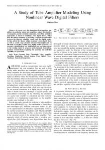
Figure 1: Basic WDF one-port elements: (a) a generic one-port, (b) resistor: Rp = R, (c) capacitor: Rp = T /2C, (d) inductor: Rp = 2L/T , (e) voltage source: Rp = R. Here T is sample period. Fig. 1(a) characterizes a generic LTI one-port element in the electrical domain, for which the Kirchhoff variables (for short, Kvariables) are voltage u and current i. The WDF theory maps these to wave variables (for short, W-variables) a and b at the port by relations (  u=a+b a = (u + Rp i)/2 (1) ⇔ i = (a − b)/Rp b = (u − Rp i)/2 where a is the incident (in-coming) and b the reflected (out-going) wave component, and Rp is a free parameter called port resistance. While the relation between the two K-variables in a linear system is given by impedance Z = U/I (capital letters from now on denote Laplace or z-transform variables), the behavior of a wave port is described by its reflectance H = B/A = (Z − Rp )/(Z + Rp ). Classical WDFs are derived from analog prototypes by the bilinear mapping [7], which preserves energetic properties of the prototype analog system such as passivity, being important from the stability point of view. By proper values for the port resistance Rp to avoid delay-free loops in computation, realizations of basic WDF elements are easily derived [2] as shown in Fig. 1(b-e) for the resistor, capacitor, inductor, and voltage source. Adaptors are WDF multi-port elements that are needed to construct circuit and network models from the basic elements [2]. The task of an adaptor is to realize the scattering of wave variables among the ports connected together. Fig. 2 shows the parallel and series circuit connections in (a) and (c), and the symbols for parallel (b) and series (d) adaptors, respectively. Adaptors are constructed so that for a single port, say port N , the output BN is independent of its input AN . This is called a reflection-free port because BN can be read before knowing the new value of AN , which cannot be done for the other ports, see Fig. 2(b). Such a reflection-free port can be used without computability problems for further connections in a network. Adaptors are typically applied as 3-port elements, whereby two one-port elements are connected in parallel or series, and the

DAFX-1

Proc. of the 12th Int. Conference on Digital Audio Effects (DAFx-09), Como, Italy, September 1-4, 2009

Figure 2: Parallel and series adaptors: (a) parallel connection for K-variables, (b) WDF symbol for wave variables, including reflection-free port N marked by terminal >. Corresponding cases for series adaptor: (c) and (d).

Figure 3 illustrates the electrical equivalent circuit of the output chain. The equivalent circuits for the mechanical and acoustical parts of the loudspeaker are found by using the well-known analogies between electrical, mechanical, and acoustic systems, see, e. g. [5]. It must be noted that although the mechanical and acoustical systems are represented as electronic components in Fig. 3, their physical quantities (e. g. mass and compliance of the loudspeaker) are still directly controllable. Numerical values for the components in Fig. 3 are listed in Table 1. Table 1: List of components and their values used in Fig. 3. Symbol Value Explanation Vi Input signal source Ci 100 nF Input capacitance Ri 1 MΩ Input resistance Rg 20 kΩ Grid resistance Rk 20 Ω Cathode resistance Ck 10 µF Cathode capacitance V+ 500 V Operating voltage source R+ 1Ω Voltage source resistance Rp1 131 Ω Transf. primary resistance 1 Rp2 9.2 kΩ Transf. primary resistance 2 Lp 7.6 H Transf. primary inductance Tee N = 28 Ideal electrical transf. Rs1 8Ω Transf. secondary resistance 1 Rs2 225 Ω Transf. secondary resistance 2 Ls 8.2 mH Transf. secondary inductance Cs 145 nF Transf. secondary capacitance Re 6.95 Ω Loudsp. resistance (electric) Le 690 µH Loudsp. inductance (electric) Tem N = 8.3 Ideal electromechanical transf. Rm 1Ω Loudsp. resistance (mechanic) Cm 27 mF Loudsp. capacitance (mechanic) Lm 560 µH Loudsp. inductance (mechanic) Tma N = 1/0.0204 Ideal acoustomechanical transf. Ca 398 mF Loudsp. capacitance (acoustic) Ra 122 µΩ Loudsp. resistance (acoustic)

third port of the adaptor is further connected in parallel or series with something else, etc., up to a short or open circuit termination or a special root element. Therefore such a circuit structure appears as a tree-structure, in the particular case of 3-port adaptors as a binary tree. Several types of general two-port elements are available for construction of WDF circuits and networks. Only the ideal transformer is needed in this article. It is realized simply by wave variable scalings B2 = N A1 and B1 = (1/N )A2 where A1 and B1 are wave variables at port 1, A2 and B2 at port 2, and N is the turns ratio. The port resistances have to be scaled by Rp2 = N 2 Rp1 . Modeling of nonlinearities The basic WDF theory as such is valid only for modeling of LTI circuits, while nonlinearities bring challenges with aliasing and computability. Aliasing is a common problem in nonlinear DSP and computability problems are related to avoidance of delayfree loops. While in LTI circuits the port resistances are constantvalued, in a nonlinear element the port resistance becomes a function of the wave variables at the port. However, the wave variables depend on the port resistance, so we have an implicit set of equations, which in a general case has to be solved by iteration. Furthermore, the rest of the binary tree up to the root needs to take part in the iteration. A special case is a single nonlinearity used as the root element, whereby its effect is localized, and the nonlinearity can be formulated simply as a nonlinear wave-port reflection function B = f (A). Since full iteration of wave-port elements is computationally expensive and complicated, in practice a delay-free loop can often be cut by inserting an extra unit delay, e.g., by using a delayed value of port resistance. This invalidates the energetic passivity rule, so that instabilities may quite easily appear, often at the Nyquist frequency (half of the sampling rate). Oversampling is typically needed to minimize the problem, but this may be a necessity in nonlinear DSP anyway, and helps also in cases where the frequency-warping due to bilinear mapping in WDFs [2] is a problem. 3. THE OUTPUT CHAIN The output chain of a typical single-ended triode power amplifier consists of an RC-circuit containing one triode tube, an output transformer, and a loudspeaker. In a nutshell, the tube circuit, called power amp stage, creates a nonlinear voltage-to-current amplification. The output transformer applies an impedance transform between the tube (high impedance) and the loudspeaker (low impedance), so that electric power is efficiently transmitted to the loudspeaker. Naturally, the loudspeaker then transmits the power from the electrical domain first into the mechanical, and then into the acoustical domain.

3.1. Single-ended triode power stage The tube power amplifier stage is illustrated in the leftmost part of Fig. 3. The amplifier uses only one triode tube for amplifying the signal, hence the name "single-ended triode stage". Basically, the tube element provides nonlinear phase-inverting amplification between the grid (denoted with g) and the plate (denoted with p) terminals. More detailed discussion on the function of the different RC components of the stage is presented in [3]. 3.2. Output transformer A transformer is a device that transforms electrical energy from one circuit to another. With amplifiers, the output transformer couples the loudspeaker to the output stage of the amplifier. As an electric load, seen by the amplifier, the transformer multiplies the impedance of the load (loudspeaker) by the square of the transformation ratio. The transformation ratio, for ideal transformers, is given by the ratio of the turns in the coils. However, real transformers are far from ideal ones. In practical transformers there are various mechanisms introducing losses in the transformation. This affects the load seen by the amplifier. The equivalent circuit model for the output transformer, illustrated in Fig. 3, was devised after measuring a typical output transformer,

DAFX-2

Proc. of the 12th Int. Conference on Digital Audio Effects (DAFx-09), Como, Italy, September 1-4, 2009

Figure 3: The electrical equivalent circuit of the power amplifier stage, output transformer, and the loudspeaker. Note that the transition between different domains (electrical, mechanical, acoustical) as well as the output transformer itself is implemented using ideal transformers. The component values are listed in Table 1. used in a low wattage single-ended tube amplifier. More specifically, the transformer model used in the circuit was based on an equivalent circuit model in [8], and then modified to fit the open circuit load measurement results conducted on the physical transformer. In other words, the model mimics the impedance seen in the primary when the secondary circuit is open (and vice versa). Figure 4 illustrates the measured open load impedances and the results obtained from the model in Fig. 3. It is important to note, however, that although the simulation results in Fig. 4 show a good match to the measured data, the open circuit load differs from a load of a loudspeaker, and this is thus still a relatively rough approximation of a real transformer. 4

Impedance (Ohm)

10

3

10

2

with ideal transformers. All of the components in different domains have an effect on the electric impedance seen by the amplifier driving the loudspeaker. The voice coil can be modeled [9] with an ideal transformer Tem , in series with coil inductance Le and resistance Re . The transformation ratio of Tem is given by the Bl-factor, where B is the magnet field strength in the voice coil gap, and l is the length of the wire in the magnetic field. Using the mobility analogy, the cone movement in the mechanical domain is modeled as a parallel RCL circuit, where Cm equals the mass of the cone and the voice coil, Lm is the compliance of the attachment, and Rm is the damping caused by the attachment. The loudspeaker parameters given in Table 1 were estimated from an Eminence Guitar Legend 121 loudspeaker using measurements and the information given in the loudspeaker’s datasheet. Eventually, the cone is coupled to the air via transformer Tma with a transformation ratio equivalent to the inverse of the cone surface area. The radiation impedance seen by the cone is modeled as a series RC circuit.

10

1

10

4. WAVE DIGITAL FILTER MODEL 2

10

3

10

10

4

Frequency (Hz)

Figure 4: Impedance curves for the measured (solid line) and simulated (circles) output transformer. The upper plot illustrates the open load impedance as measured from the primary, while the lower plot shows the open load impedance as measured from the secondary. 3.3. Lumped model of the loudspeaker A loudspeaker transforms the electric signal to pressure changes in the air, which can be heard as sound. A typical moving-coil loudspeaker consist of a voice coil which is attached to a rigid cone. The voice coil and the cone are attached to the frame of the loudspeaker by a "spider" underneath the cone, and by the surroundings of the cone. To enable the axial movement of the coil, (in order to produce sound) the attachment has to be made flexible. The voice coil is placed in a magnetic field, and therefore acts as an electric motor to drive the cone. When a time varying signal is fed to the voice coil, the cone tries move accordingly, thus producing pressure waves in front of the cone, which ultimately can be heard as sound. As a lumped model, the loudspeaker can be divided into three different domains: electrical (voice coil), mechanical (cone mass and attachment), and acoustical (sound radiation). The separation between the domains can be implemented

The WDF structure corresponding to the circuit of Fig. 3 is illustrated in Figure 5. It consists of six sub-blocks, namely the grid-, plate-, and cathode circuits, the three-port triode tube itself, the output transformer, and the loudspeaker block. The nonlinear tube element is chosen as the root block here, so all the reflection-free ports of the network point toward the WDF tube. As stated in Sec. 1, the power amp model is based on the improved WDF tube stage model presented in [3]. The advantage of using this model over the previous WDF tube stage model [4] is that due to the correct simulation of grid current, the coupling between the grid and the cathode (and thus the rest of the circuitry) is taken into account. The triode model parameters are chosen so that the model represents a KT88 power tetrode strapped in triode operation. For a KT88 datasheet, see e. g. [10]. The WDF structures of the output transformer and the loudspeaker are illustrated in Fig. 5 with the corresponding blocks. Due to the flexible nature of the WDF technique, each of the component values can be made adjustable in real-time. For usability purposes, however, it might be best to limit the amount of adjustable parameters by defining compound variables, such as loudspeaker size. For example by adjusting the size of the loudspeaker, the user would actually change both the mass of the cone (Cm ) and the area of the cone surface (transform ratio of Tma ).

DAFX-3

Proc. of the 12th Int. Conference on Digital Audio Effects (DAFx-09), Como, Italy, September 1-4, 2009

Figure 5: WDF network representing the circuit in Fig. 3. Details of the WDF tube model are presented in [3]. 4.1. Real-time implementation

(a)

IRa (A)

1

0

Simulation results were obtained by inserting an excitation signal to the input voltage source Vi , and recording the current through the acoustical resistance Ra . The input voltage corresponds to the signal obtained from a preamplifier circuit, while the current through Ra corresponds to the sound pressure (in Pascals) at the loudspeaker. For verifying the correct operation of the WDF model, the same circuit was modeled using the LTSpice [12] non-real-time circuit simulation software, using the modified trapezoidal integration method. Figure 6(a) illustrates the current through the acoustical resistance Ra when a sinusoidal logarithmic sweep from 20 Hz to 5 kHz and amplitude of 16 V is inserted as the input signal Vi . The result from the WDF model implemented with the BlockCompiler is drawn with a solid black line. The output from the LTSpice is drawn with dashed gray line. Figure. 6(b) plots the root-meansquare difference of the WDF and LTSpice simulations. As can be seen, the simulation results are nearly identical, especially for low frequencies. In Fig. 6(a), the maximum amplitude of 1.3 A (equivalent to 1.3 Pascals) corresponds roughly to the sound pressure level of 96 dB. The linear magnitude response of the WDF output chain (from Vi to Ra ) is illustrated in Figure 7, together with the magnitude response curves of the 2nd and 3rd harmonic distortion components. A logarithmic sine sweep from 20 Hz to 10 kHz with the amplitude of 16 V was used as an input signal, and the linear and distorted responses were evaluated from the output signal [13]. Sound samples of an electric guitar played through the WDF output chain will be available at http://www.acoustics. hut.fi/publications/papers/dafx09-wdf.

0.2

0.4

0.6

0.8

1

0.6

0.8

1

Time (s) (b)

−8

10

−10

10

0

0.2

0.4 Time (s)

Figure 6: The output signals (a) of the WDF model (solid black line) and a reference model, implemented with LTSpice (dashed gray line), when a logarithmic sine sweep from 20 Hz to 5 kHz is used as an input signal. The root-mean-square difference between the WDF and LTSpice simulations is illustrated in (b). As can be seen, the simulation results are nearly identical.

Linear

0 Magnitude (dB)

5. SIMULATION RESULTS

0 −1

RMSE (dB)

The real-time model is implemented with the BlockCompiler [11] software. It runs at 44100 Hz sampling frequency on a 2.4 GHz MacBook (Intel Core 2 Duo) with an external M-Audio Firewire 410 audio interface. The model consisting of the power amp circuit, transformer, and the loudspeaker presented in Fig. 5 consumes approximately 2.1 % of CPU time. As suggested in [4], a lookup-table implementation of the vacuum-tube would result in an even smaller CPU load.

−20 3rd harm. 2nd harm.

−40 −60

100

1k Frequency (Hz)

10k

Figure 7: The linear magnitude response and the 2nd and 3rd harmonic distortion components of the WDF output stage. A logarithmic sine sweep with amplitude of 16 V was used as the input signal.

DAFX-4

Proc. of the 12th Int. Conference on Digital Audio Effects (DAFx-09), Como, Italy, September 1-4, 2009 6. CONCLUSIONS AND FUTURE WORK

[5] V. Välimäki, J. Pakarinen, C. Erkut, and M. Karjalainen, “Discrete-time modelling of musical instruments,” Reports on Progress in Physics, vol. 69, no. 1, pp. 1–78, Jan. 2006.

A WDF model for simulating the combination of a single-ended triode power amplifier stage, output transformer, and a loudspeaker, was presented. The nonlinear power amplifier stage model was derived from a triode stage model, presented in [3]. The linear output transformer model was devised according to electrical measurements on a real output transformer. Also, the loudspeaker parameters were measured from a real guitar loudspeaker. A real-time model is implemented using the BlockCompiler software. The real-time simulation results were verified using the LTSpice circuit simulation software. Improving the transformer model by fitting it to a more realistic load and modeling also the nonlinearities in the transformer and loudspeaker remains as future work.

[6] J. O. Smith, Physical Audio Signal Processing: Digital Waveguide Modeling of Musical Instruments and Audio Effects, 2004, Dec. 2008 Edition, available on-line at http://ccrma.stanford.edu/ ~jos/pasp/, accessed Jun. 25, 2009. [7] John G. Proakis and Dimitris G. Manolakis, Digital Signal Processing — Principles, Algorithms, and Applications, Pearson Prentice Hall, New Jersey, USA, Fourth Edition, 2007. [8] “Transformer,” 2009, Internet article, available online at http://en.wikipedia.org/wiki/ Transformer, accessed Jun. 24, 2009.

7. ACKNOWLEDGMENTS This research is funded by Helsinki University of Technology.

[9] L. Beranek, Acoustics, American Institute of Physics, New York, USA, Third printing, 1988.

8. REFERENCES [1] J. Pakarinen and D. T. Yeh, “A review on digital guitar tube amplifier modeling techniques,” Computer Music J., vol. 33, no. 2, pp. 85–100, 2009, Available on-line at http://www.mitpressjournals.org/ doi/pdf/10.1162/comj.2009.33.2.85, accessed Jun. 25, 2009. [2] A. Fettweis, “Wave digital filters: Theory and practice,” Proc. IEEE, vol. 74, no. 2, pp. 270–327, Feb. 1986. [3] J. Pakarinen and M. Karjalainen, “Real-time physical modeling of tube stage circuits,” IEEE Trans. on Audio, Speech, and Language Processing, 2009, Submitted for publication. [4] M. Karjalainen and J. Pakarinen, “Wave digital simulation of a vacuum-tube amplifier,” in Proc. Intl. Conf. on Acoustics, Speech, and Signal Proc., Toulouse, France, May 15-19 2006.

[10] “Genalex KT88,” 1974, Tube datasheet, available on-line at http://www.drtube.com/datasheets/ kt88-mov74.pdf, accessed Jun. 25, 2009. [11] M. Karjalainen, “BlockCompiler: Efficient simulation of acoustic and audio systems,” in Proc. 114th AES Convention, Amsterdam, The Netherlands, Mar. 22-25 2003. [12] Linear Technology, “SwitcherCAD III / LTSpice Users Guide,” 2009, Available online at ltspice.linear. com/software/scad3.pdf, accessed 19 February 2009. [13] A. Farina, “Simultaneous measurement of impulse response and distortion with a swept-sine technique,” in Proc. 108th AES Convention, preprint 5093, Paris, France, Feb. 19-22 2000.

DAFX-5