Stanford Exploration Project, Report 112, November 11, 2002, pages 21–27
Short Note Wave-equation MVA using diffracted data Paul Sava and John Etgen1
INTRODUCTION Migration velocity analysis (MVA) using diffracted data is not a new concept. Harlan (1986) addressed this problem and proposed a method to isolate diffraction events around faults. He also proposed a MVA technique applicable to simple geology, constant velocity or v(z), and quantifies the focusing quality using statistical tools. de Vries and Berkhout (1984) use the concept of minimum entropy to evaluate diffraction focusing, and apply this methodology to MVA, again for the case of simple geology. Biondi and Sava (1999) introduce a method of migration velocity analysis using waveequation techniques (WEMVA), which aims at improving the quality of migrated images, mainly by correcting moveout inaccuracies of specular energy. The slowness model is estimated by finding the slowness perturbation which explains the difference between the migrated image using the reference model and an externally-defined target image (Sava and Symes, 2002). The moveout information given by the specular energy is not the only information contained by an image migrated with the incorrect slowness. Non-specular diffracted energy is present in the image and clearly indicates slowness inaccuracies. Since a difference between an inaccurate image and a perfectly focused target image contains both specular and nonspecular energy, WEMVA is naturally able to derive velocity updates based on both these types of information. In contrast, traveltime-based MVA methods cannot easily deal with the diffraction energy, and are most of the time concerned with moveout analysis. In this paper, we examine the resolving power of the unfocused diffraction energy present in migrated images. The target applications of these techniques are in areas of complicated geology in which diffractions are abundant and can be clearly identified and isolated. Examples include highly fractured reservoirs, carbonate reservoirs, rough salt bodies and reservoirs with complicated stratigraphic features. Of particular interest is the case of salt bodies. Diffractions can help estimate more accurate velocities at top of salt, particularly in the cases of rough salt bodies. Moreover, diffraction 1 email:
[email protected],
[email protected]
21
22
Sava and Etgen
SEP–112
energy may be the most sensitive velocity information we have under salt, since most of the reflected energy we record at the surface has only a narrow range of angles of incidence at the reflector, rendering the analysis of moveout useless.
METHODOLOGY In its original formulation (Biondi and Sava, 1999), wave-equation migration velocity analysis relates a perturbation of the slowness model (1S) to its corresponding perturbation of the seismic image (1R). Mathematically, this relation can be expressed as the linear fitting goal L1S ≈ 1R.
(1)
L is the WEMVA operator and is constructed as a linearization of downward continuation operators involving the Born approximation (Sava and Fomel, 2002). We obtain the slowness perturbation 1S from Equation (1) by applying either the adjoint or the least-squares inverse of L to the image perturbation 1R. The critical quantity in Equation (1) is the perturbation of the seismic image 1R. For the purpose of this equation, this is the known quantity and various techniques can be used to derive it. Suppose we can isolate all the diffractions from a given dataset. The migration velocity is correct if all diffractions are focused, both as a function of space and as a function of offset. Any inaccuracy of the velocity model leaves undiffracted energy in the image. This simple observation gives us a mechanism to define image perturbations usable for WEMVA. First, we migrate the data using the reference slowness model and obtain a reference image R0 . Second, we correct all unfocused diffractions using a residual technique (residual migration for example), and obtain an improved image R. Finally we take the difference between R and R0 as the image perturbation 1R, which can be inverted for slowness perturbation 1S using Equation (1). This method is in principle usable for diffraction data analyzed in a prestack volume. However, as we will demonstrate with the example in the next section, a substantial part of information usable for MVA is present in the zero offset section. Our example concerns WEMVA purely at zero offset with the goal of isolating focusing effects from moveout-based effects.
EXAMPLE We illustrate this diffraction focusing technique with a synthetic model simulating the diffracting points at the top of a rough salt body. The model is depicted in Figure 1: the reflectivity at the top, and the reference slowness in the middle. The model consists of several diffractions, and the reference slowness is smoothly spatially varying.
SEP–112
Diffraction WEMVA
23
Figure 1 shows at the bottom the image perturbation 1R caused by the ideal slowness perturbation 1S shown in the top panel in Figure 2. 1R is created by subtracting the reference image from the perfectly focused one 1R = R − R0 . We take the image perturbation shown in the bottom panel of Figure 1 and compute the corresponding slowness perturbation using Equation (1). Figure 2 shows in the middle the result we obtain by applying the adjoint of the operator L to the image perturbation in Figure 1, and at the bottom the result of applying the least-squares inverse of L to the same 1R. Despite the inherent vertical smearing caused by the limited angular coverage, the slowness perturbations are nicely focused at their correct locations. Obviously, the result obtained with the least-squares inverse is much better focused than the one obtained by the simple adjoint operator, although we have only used the zero-offset and not the entire prestack data. The simple backprojection (top panel in Figure 2) creates “fat rays,” also discussed by Woodward (1992) and Sava (2000).
CONCLUSIONS We present an application of the WEMVA methodology to diffracted seismic data. Diffractions carry a substantial amount of velocity information which is largely ignored by the current MVA techniques. We show that diffractions can be used for accurate migration velocity analysis using the WEMVA methodology. In the current form, the limitations of this method are identical to those of WEMVA, and are mainly related to the Born approximation assumed by the method which requires small perturbations. Further extensions are possible, but they remain subject to future research.
ACKNOWLEDGMENT This work was performed during the first author’s internship at BP Upstream Technology Group.
REFERENCES Biondi, B., and Sava, P., 1999, Wave-equation migration velocity analysis: SEP–100, 11–34. de Vries, D., and Berkhout, A. J., 1984, Velocity analysis based on minimum entropy: Geophysics, 49, no. 12, 2132–2142. Harlan, W. S., 1986, Signal-noise separation and seismic inversion: Ph.D. thesis, Stanford University. Sava, P., and Fomel, S., 2002, Wave-equation migration velocity analysis beyond the Born approximation: SEP–111, 81–99.
24
Sava and Etgen
SEP–112
Sava, P., and Symes, W. W., 2002, A generalization of wave-equation migration velocity analysis: SEP–112, 27–36. Sava, P., 2000, A tutorial on mixed-domain wave-equation migration and migration velocity analysis: SEP–105, 139–156. Woodward, M. J., 1992, Wave-equation tomography: Geophysics, 57, no. 1, 15–26.
Figure 1: Synthetic model: reflectivity (top), background slowness (middle), and image perturbation (bottom). paul2-imags [CR]
SEP–112
Diffraction WEMVA
25
Figure 2: Ideal slowness perturbation (top), Slowness perturbation obtained by the adjoint of L (middle) and by the least-squares inverse of L (bottom) applied to the image perturbation in Figure 1. paul2-slows [CR]
26