the increase of ¯ky, more band gaps appear, some of which will disappear with ¯ky increasing. For instance, the band gap near L1 =3 65 appears when ¯ky =0 ...
Copyright © 2013 American Scientific Publishers All rights reserved Printed in the United States of America
Journal of Computational and Theoretical Nanoscience Vol. 10, 2427–2437, 2013
RESEARCH ARTICLE
Wave Propagation in Nanoscaled Periodic Layered Structures A-Li Chen, Yue-Sheng Wang∗ , Liao-Liang Ke, Ya-Fang Guo, and Zheng-Dao Wang Institute of Engineering Mechanics, Beijing Jiaotong University, Beijing 100044, China In this paper the propagation of elastic waves in nanoscaled periodic layered structures is studied by using the nonlocal elastic continuum theory. The localization factor is introduced to describe the band structures for waves propagating either normally or obliquely in the system. Both the anti-plane and mixed in-plane wave modes are considered with detailed computations being performed for the nanoscaled HfO2 –ZrO2 periodic layered structures. The localization factors as well as the dispersion curves are calculated to analyze the size-effect on the behaviors of the wave propagation. A cutoff frequency is found, beyond which waves cannot propagate through the system. The influences of the ratio of the internal to external characteristic lengths on the cut-off frequency and band structures are discussed. The generation and behavior of the band gaps with or without the mode conversion are also analyzed for the mixed in-plane wave modes.
Keywords: Elastic Wave, Layered Structure, Superlattice, Phononic Crystal, Size-Effect, Nonlocal Elastic Theory, Localization Factor.
Delivered by Publishing Technology to: University of New South Wales IP: 149.171.67.164 On: Sat,in15 Jun 2013 00:23:31 periodic layered piecewise-homogeneous composites. Copyright: American Scientific Publishers These results can be found in a review paper written by The studies on the elastic wave propagation in the layered Guz’ and Shulga14 in which the elastic wave propagation medium, which found their original motivation in studies in laminated and fibrous unidirectional composite materiof the wave propagation of seismic shocks through the als modeled by the piecewise-homogeneous medium was earth’s crust and the acoustic waves in the atmosphere or concerned. In this review paper, a detailed comprehensive the water, have more than 50 years. The previously pubanalysis was given for bulk, surface and normal waves lished fewer works on multilayered isotropic media can propagating in the laminated materials. The structure of be found in the books by Ewing et al.1 Brekhovskikh2 the pass band zones for shear and longitudinal-transverse and Kennerr.3 For systems consisting of layered periodic bulk waves was described with its dependence of the relmedia, we mention the work of Rytov,4 who studied a ative thickness and mechanical properties of layers. bilayered periodic medium for the purpose of obtaining With the rapid development, the lucubration and the effective mechanical properties for “thinly layered syswidely usage of the semiconductor, the attention of the tems.” Hegemier and Nayfeh5 studied a similar model and scientific world has been focused on artificial superpederived exact and asymptotic results for the propagation of riodic structures called superlattices which are grown waves having arbitrary frequencies in such a system. Subfrom semiconductor or metallic layers.15 Many researches sequently, Nayfeh6 generalized the results of Ref. [5] to the were reported on elastic or acoustic wave propagation case of multilayered media. Nemat-Nasser7 and Nematin superlattices. Saperiel and Djafari Rouhani16 presented Nasser et al.8� 9 studied harmonic waves in a variety of a comprehensive survey, both theoretical and experimencomposites consisting of isotropic layers. As compared tal, of the vibration modes in superlattices. The propagawith isotropic cases, solutions to the anisotropic probtion of the bulk or surface acoustic waves, the coupling lem are much more difficult to obtain. Nayfeh10 used the of the optical and acoustic waves and the wave propmatrix transfer method and presented solutions for genagation in the piezoelectric superlattices were discussed erally polarized waves on multilayered anisotropic media, in detail; and the calculation methods of the dispersion respectively. Shulga and his coauthors did many researches relations were stated clearly. Usually the transfer matrix on elastic,11 electroelastic12 and magnetoelastic13 waves method can be used to obtain the dispersion relations of the bulk (and also of the surface) acoustic waves in the ∗ Author to whom correspondence should be addressed. superlattices.17–19 Besides the transfer matrix method, the
1. INTRODUCTION
J. Comput. Theor. Nanosci. 2013, Vol. 10, No. 10
1546-1955/2013/10/2427/011
doi:10.1166/jctn.2013.3225
2427
RESEARCH ARTICLE
Wave Propagation in Nanoscaled Periodic Layered Structures
Chen et al.
dispersion relations can also be obtained by using differsemiconductors by using the ball-and-spring model. For ent formulations of the Green’s function method17� 20–22 or two-dimensional phononic crystals, Zhen et al.59 and Liu 23 the interface response theory. A formal generalization of et al.60 studied the surface/interface effects on the band the above methods to a superlattice composed of N difstructures. The results showed that the surface effect on ferent layers (instead of two) was reported.24� 25 Besides the band structure would be significant as the characteristic the periodic superlattices, Merlin et al.26 demonstrated the size reduces to nanometers. possibility of artificially fabricating one-dimensional (1D) In this paper the elastic waves propagating normally and quasi-crystalline structures. The propagation of acoustic obliquely in the 1D nanoscaled periodic layered structures waves in quasi-periodic Fibonacci superlattices was studare studied by using the nonlocal elastic (NLE) continied both theoretically and experimentally27� 28 and showed uum theory.61 The NLE theory includes the effects of the the general behaviour expected in a 1D quasi-crystal. long range interatomic forces by supposing that the stressSince the conception of phononic crystals (PNCs), state at a point is related to the strain-state at all points a kind of composites composed of periodic arrays of two of the entire body. Artan et al.62 studied the dispersion or more materials with different mass densities and elasbehaviors of shear waves propagating in periodic layered tic properties, was first proposed by Kushwaha et al.29 media with nonlocal effects. Recently this theory has been in 1993, the propagation of the classical elastic waves successfully used to analyze the mechanical behaviors of along the periodical structures recalled the attentions of nanoscaled structures where the size-effects must be taken the researchers. The most important property of PNCs is into account.63–70 In fact we have applied the NLE thethe band gaps which have numerous potential engineering ory to study the shear wave propagating normally in the applications such as wave detectors, filters, waveguides, 1D nanoscaled HfO2 –ZrO2 PNC.71 The first two bands of transducers, acoustic lenses, acoustic interferometers, etc. the dispersion curves were calculated and compared with It is known that the 1D PNC is actually the periodic laythe results from the first-principles method.55 The results ered structures. In fact, the band gaps or stop bands have show that the developed NLE method is expected to overbeen found for a long time for wave propagation in the come the limits of the CE description for wave propagaperiodic layered structures.14 Many results were reported tion in periodic layered structures when dimensions are for elastic waves propagating in the 1D ordered, defected, in nanometer-length scales. In this paper the conception piezoelectric and viscoelastic PNCs (i.e., periodic layered of the localization factors72 are introduced to describe the Delivered Publishing Technology University of for New South Wales either normally or someby results for wave propa- to: composites).30–38 Recently, band structures waves propagating IP: 149.171.67.164 On: Sat, 15 Jun 2013 00:23:31 gation in the 1D randomly disordered and quasi-periodic obliquelyPublishers in the nanoscaled system. Both the anti-plane Copyright: American Scientific PNCs were also presented.39–42 and mixed in-plane wave modes are considered. The localWith the rapid development of the technology in the ization factors as well as the dispersion curves are calcufields of communication information, medical engineerlated to analyze the behaviors of the wave propagation. ing, etc., the size of acoustic devices is required to be A cut-off frequency is found, beyond which waves cannot smaller and smaller. For instance, the gigahertz commupropagate through the system. The influences of the ratio nication generally requires the nanosized devices. The of the internal to external characteristic lengths on the cuthypersonic phononic band gaps could be used to design off frequency and band structures are discussed. The gennew thermo-electric devices, acoustic-optic devices, nano eration and behavior of the band gaps with or without the electric-mechanical systems (NEMS), etc.43–48 Recently, mode conversion are also analyzed for the mixed in-plane the manufacture, measurement and computation of the wave modes. hypersonic PNC together with its applications in manipulation of hypersonic acoustic waves have received more and more considerable attention.49–52 2. PROBLEM STATEMENT AND It is known that the size-effect53� 54 will become FORMULATION more important and should be taken into account when Consider a periodic layered structure consisting of layers a system is in the dimension of several nanometers. (sub-cells) A and B alternatively as shown in Figure 1. Ramprasad et al.55 calculated the phononic band strucThe thickness of the layers A and B, which denoted as d1 tures for a nanoscaled multilayer stack by using the firstand d2 , are at the nanoscale. The global and local coorprinciples method56 at the atomistic level and by solving dinate systems at each layer are established, see Figure 1. the classical elastic wave equation at the continuum level, In this paper, we consider plane waves propagating in an respectively. They found that the results calculated by arbitrary direction. The wave fields are the functions of x using the two methods are quite different and pointed out and y, so the problem considered is a two-dimensional that the scaling law57 does not work when the sizes of (2D) problem. the PNCs are in the nanoscaled dimension. Hepplestone Unlike the CE theory which assumes that the stress at et al.58 also highlighted the limits of the classical elasa point is solely dependent on the local strain field at tic (CE) continuum theory when they studied the hypersonic phonon modes in periodically arranged composite this point, the NLE theory takes into account the effects 2428
J. Comput. Theor. Nanosci. 10, 2427–2437, 2013
Chen et al.
Wave Propagation in Nanoscaled Periodic Layered Structures y
θ0
x
incident waves
A
B
d1
d2
The kth unit cell
Fig. 1. Schematic diagram of a one-dimensional periodic layered structure, the size of the structure is at the nanoscale.
of the long range interatomic forces and supposes that the stress-state at a point is related to the strain-state at all points of the entire body. By introducing the concept of the influence function �, the constitutive relations are written as61 � �kl �x� = ���x� − x���kl �x� � dv�x� �� k� l = 1∼3 (1) V
where x is the position vector; �kl are the nonlocal stress components; and �kl are the stress components calculated by the CE theory which, for the homogeneous and isotropic medium, are given by �
�
�
�kl �x � = �err �x � kl + 2 ekl �x �
(2)
�1 − 2 � 2 ��kl = �kl
(7)
Then the dynamic equilibrium equation without body forces is (8) � �� = �u¨ � with � being the mass density. Substitution of Eqs. (2), (3) and (7) into Eq. (8) yields the following differential wave motion equation of the NLE theory: �� + �u � � + u��
= �1 − 2 � 2 ��u¨ �
(9)
where � = � /�x + � /�y is the Laplace operator. For the present 2D problem we introduce two displacement potentials, � and �, such that the displacement components, ux and uy , are written as73 2
2
2
ux =
2
2
�� �� + � �x �y
uy =
�� �� − �y �x
(10)
Then the governing wave motion equation, i.e., Eq. (9), can be decoupled into the following equations:74 cL2 � 2 � − �1 − 2 � 2 ��¨ = 0 cT2 � 2 � − �1 − 2 � 2 ��¨ = 0
(11)
where cL and cT are, respectively, � Technology to: � � Wales the classical √phase � Delivered Publishing University of New South 1 �uk �x� �by �u l �x � = �� + 2 �/� and cT = /�. velocities defined by c L (3) Sat, 15 Jun 2013 00:23:31 + 149.171.67.164 ekl �x � = IP: On: � 2 �xl� �x For the in-plane harmonic wave propagating in an arbik Copyright: American Scientific Publishers trary direction �0 with the y-component of the wave vector where � and are Lamé constants for the correspondbeing ky = k0 sin �0 = � sin �0 /c0 , if the Snell law is coning classical elasticity;61 and uk are the displacement sidered, � and � have the following forms: components; and ���x� − x�� is the influence function which is dependent on the internal characteristic length ��x� y� t� = ��x� exp�iky y − i�t� (e.g., the atomic lattice constant). It is noted that �kl = �kl (12) ��x� y� t� = � �x� exp�iky y − i�t� when ���x� − x�� is a delta function ��x� − x��. Detailed properties of ���x� −x�� and the determination of its particIt will be convenient to cast the equations into dimensionular form may be found in Ref. [61]. Here for the layered less forms by introducing the dimensionless local coordistructures the dimension in y-direction is infinite and thus nates: no scale effect will be considered in this direction. There(13) �j = xj /d� �j = yj /d fore we take the influence function ���x� − x�� for the 2D where j = 1, 2 represent for the jth sub-layer; d = d1 +d2 ; system in this paper as d� and 0 ≤ �j ≤ d¯j = dj /d. Then the general dimensionless � � � ���x − x�� = ���x − x�� ��y − y�� (4) harmonic displacement potentials-solutions for the inplane waves propagating in the jth sub-cell have the folwith ���x� − x�� being the influence function along lowing forms: the x-direction. Then the constitutive relations can be ¯ �j = �A1j e−iqLj �j + A2j eiqLj �j �eiky �j −i�t written as (14) � ¯ �j = �B1j e−iqTj �j + B2j eiqTj �j �eiky �j −i�t � � �x� = ���x� − x��� � �x� � ds�x� � s where k¯ y = ky d; and � +� � di � � � � � � = ���x − x�� ��y − y��� � �x � dx dy (5) −� 0 �¯ 2 = − k¯ y2 q Lj �cLj /cL1 �2 − R2j �¯ 2 The explicit form of ���x� − x�� may be found in Ref. [61]. � Here we select it to be �¯ 2 1 � qTj = − k¯ y2 ��x −x��/ � ���x − x�� � = e (6) �cTj /cL1 �2 − R2j �¯ 2 2 with
�
J. Comput. Theor. Nanosci. 10, 2427–2437, 2013
2429
RESEARCH ARTICLE
o1
which, when → 0, reduces to the delta function ��x� − x��. The constitutive equation of the integral form, Eq. (1), can be approximated by a differential one:61
y1 y2 x 1 x2
y1y2 x1 x2
Wave Propagation in Nanoscaled Periodic Layered Structures
RESEARCH ARTICLE
with �¯ = �d/cL1 and Rj = j /d. The dimensionless displacement and stress components are given by �� �� �� �� + � u¯ y = − �� �� �� �� � � � 2 � 2 � � � � �2� �2� �¯ x = � + 2
+ + �� 2 ��2 �� 2 ���� � � 2 � � �2� �2� �¯ yx = 2 − + ���� ��2 �� 2 u¯ x =
(15a)
(15b)
−�
=
d¯j 0
0
1 −��j� −�j �/Rj e �¯ xy ��j� � d�j� 2Rj
(16)
�k�
= V1L
(20)
From Eqs. (18)–(20), we can easily derive V2R = T� 2 V2L = T� 2 V1R = T� 2 T� 1 V1L �k�
�k�
�k�
�k�
�k−1� d�
= T� 2 T� 1 V2R
0
d¯j
−�
While the continuity between the two sub-cells of the kth or (k−1)th unit cell states, �k−1�
1 −��j� −�j �/Rj = e �¯ x ��j� � d�j� 0 2Rj � +� � d¯j �¯xy ��j � = ����j� − �j �� ���j� − �j ���¯ xy ��j� �d�j� d�j� �
where T�j = Nj Mj−1 is the transfer matrix of the jth subcell. The displacements and stresses are continuous at the interface between the kth and the (k−1)th unit cells, that is, �k� �k� �k−1� �k−1� V1R = V2L � V1R = V2L (19)
V2R
Then from Eqs. (5), (6) and (15b), the corresponding dimensionless nonlocal stresses �¯x and �¯xy can be obtained as � +� � d¯j �¯x ��j � = ����j� − �j �� ���j� − �j ���¯ x ��j� � d�j� d�j� �
Chen et al.
�k−1� = Tk V2R
(21)
which gives the relationship between the state vectors of the kth and the (k−1)th unit cells, where Tk = T� 2 T� 1 is the transfer matrix between the two consecutive unit cells. Because of the periodicity, Tk for all k = 1� 2� � � � are the same and denoted as T. Consider a 2m × 2m transfer matrix. In order to calculate the mth Lyapunov exponent, m orthogonal unit vectors �0� �0� of 2m-dimension, u1 � u2 � � � � � um�0� , are chosen as the initial state vectors. Eq. (21) is used to calculate the state vectors iteratively. At the kth iteration, we have
Compared with the CE theory,39 Eq. (14) involves the ratio (Rj � of the material internal characteristic length ( j � to the unit cell length (d�. The parameter Rj does reflects �k� �k−1� the influence of the nonlocal effect. It is easy to prove that = 1�2�����n�p 2R�p = Tk+1 u Delivered by Publishing Technology to:VUniversity ofp New�k South Wales = 1�2�����m� (22) 39 Eq. (14) will reduce to the resultIP: of the CE theory when 149.171.67.164 On: Sat, 15 Jun�k−1� 2013 00:23:31 where upPublishers are orthogonal unit vectors, while the vectors j → 0 (i.e., R → 0). Copyright: American Scientific �k� V2R�p (p = 1�2�����m� are usually not orthogonal. Then the following Gram-Schmidt orthonormalization procedure76 3. TRANSFER MATRIX AND is used to produce m orthogonal unit vectors LOCALIZATION FACTOR The localization factor, which is related to the Lyapunov exponent and applied to characterize the spatial evolution of a nearly periodic system, is the average exponential rate of growth or decay of the wave amplitudes.75 It has been demonstrated in Ref. [39] that the localization factor could be used to describe the band structures for wave propagation in 1D PNCs. So in this paper, we introduce the localization factor to study the wave propagation in the nanoscaled periodic layered structure. The localization factor can be calculated by following the procedure which is similar to that in Ref. [39] for the CE theory. Take V = ��¯x � �¯xy � u¯ x � u¯ y �T as the state vector. At the left and right sides of each sub-cell in the kth unit cell, we have
�k� �k� ˆ 2R�1 = V2R�1 � V
�k� ˆ 2R�1 V �k� u1 = � �k� � �V ˆ 2R�1 �
�k� �k� �k� �k� �k� ˆ 2R�2 V = V2R�2 −�V2R�2 �u1 �u1 �
��� �k� ˆ 2R�m V
�k� ˆ 2R�2 V �k� u2 = � �k� � �V ˆ 2R�2 �
���
� �k� �k� �k� �k� �k� �k� �k� = V2R�m − V2R�m �um−1 um−1 −���−�V2R�m �u1 �u1
�k� ˆ 2R�m V um�k� = � �k� � �V ˆ 2R�m �
(23)
(17)
where (·, ·� denotes the dot-product. The expression for calculating the localization factor of the system was given by Wolf:77 n 1
�k� ˆ 2R�m �m = lim ln V
(24) n→� n k=1
where the matrices Mj and Nj can be obtained from Eqs. (15a) and (16) and are given in the Appendix. Obviously, these two state vectors have the following relation:
Considering the Bloch theory which leads to V2R = �k−1� e−ikx d V2R , we can obtain the dispersion equation from the transfer matrix T,78
�k�
VjL = ��¯x � �¯xy � u¯ x � u¯ y �T�j =0 = Mj �A1j �A2j �B1j �B2j �T �k�
VjR = ��¯x � �¯xy � u¯ x � u¯ y �T� =d¯ = Nj �A1j �A2j �B1j �B2j �T j
j
d�
�k� �k� �k� VjR = Nj Mj−1 VjL = T� j VjL �
2430
j = 1� 2
(18)
�k�
�T−e−ikx d I� = 0
(25)
J. Comput. Theor. Nanosci. 10, 2427–2437, 2013
Wave Propagation in Nanoscaled Periodic Layered Structures
4. NUMERICAL RESULTS AND DISCUSSION
(a)
0.6
4.0
3.5
3.5
3.0
3.0
2.5
2.5
2.0
2.0
1.5
1.5 S wave R=0 R= 0.18
0.5 0.0 0.0
0.2
0.4
0.6
(b)
12
0.4
0.0 1.0
4.5
4.0
4.0
3.5
3.5
3.0
3.0
2.5
2.5
2.0
2.0
1.5
1.5 P wave R=0 R = 0.18
0.5 0.0
8
0.0
0.2
0.4
0.6
0.8
1.0 0.5 0.0 1.0
Delivered by Publishing Technology to: University of New South kd/π Wales IP: 149.171.67.164 On: Sat, 15 Jun 2013 00:23:31 6 Copyright: American Scientific Publishers Fig. 3. Dispersion curves for transverse (a) and longitudinal (b) waves
0.3
γ
γ
10
S wave R=0 R = 0.18
0.5
4.5
1.0 0.5
0.8
1.0
kd/π
ΩL1 = ωa/cL1
(a)
4.5
4.0
1.0
4.1. Normal Propagation In Ref. [71] we just calculated the first two bands for the transverse (T) wave propagating normally in the system.
4.5
0.2
4
0.1
2
0.0
0 0.0
0.5
1.0
1.5
2.0
2.5
3.0
3.5
4.0
4.5
ΩT1 = ωa/cT1
propagating normally in the nanoscaled periodic layered structures; the red dots and black circles represent for R = 0 and R = 0�18, respectively.
Here, the localization factors for both transverse and longitudinal (L) waves propagating normally are calculated. The thickness of the layers is dHfO2 = dZrO2 = 5�015 Å. Thus we have R1 = R2 which is denoted as R. Figures 2(a) and (b)
(b)
50
12
0.6
45 P wave R=0 R = 0.18
0.5 0.4
10
R = 0.0225
40 35
8
0.2
4
γ
6
γ
γ
30 0.3
25 20 15
2
0.1
0
0.0 0.0
0.5
1.0
1.5
2.0
2.5
3.0
3.5
4.0
4.5
ΩL1 = ωa/cL1
Fig. 2. Band structures described by the localization factors for transverse (a) and longitudinal (b) waves propagating normally in the nanoscaled periodic layered structures; the red and black circles represent for R = 0 and R = 0�18, respectively.
J. Comput. Theor. Nanosci. 10, 2427–2437, 2013
R = 0.06
10
R = 0.09 R = 0.14 R = 0.18 R=0
5 0 0
3
6
9
12 15 18 21 24 27 30 33 36 39
ΩL1/T1 Fig. 4. Influence of R on the localization factors for transverse or longitudinal waves propagating normally in the nanoscaled periodic layered structures.
2431
RESEARCH ARTICLE
Detailed calculations are performed for the propagation of both anti-plane and in-plane waves in the nanoscaled HfO2 –ZrO2 periodic layered structures. The mass densities for HfO2 (material A) and ZrO2 (material B) are 10873 kg/m3 and 6488 kg/m3 , respectively; and their transverse and longitudinal wave velocities, which were calculated by using the first-principles density functional theory in Ref. [55], are cTHfO2 = 779 m/s, cTZrO2 = 1030 m/s and cLHfO2 = 4991 m/s, cLZrO2 = 6405 m/s, respectively. In the following calculations, the internal characteristic lengths for both HfO2 and ZrO2 are assumed as 1 = 2 = 1�8054 Å which were obtained by matching the dispersion curves for bulk materials HfO2 and ZrO2 , respectively.71 The thickness of each layer is assumed the same i.e., dHfO2 = dZrO2 .
ΩT1 = ωa/cT1
Chen et al.
Wave Propagation in Nanoscaled Periodic Layered Structures
Chen et al.
30
24
cut-off frequency
18 15 12 9 6 3
0 0.00 0.02 0.04 0.06 0.08 0.10 0.12 0.14 0.16 0.18 0.20
R Fig. 5. Influence of R on the cut-off frequency for transverse or longitudinal waves propagating normally in the nanoscaled periodic layered structures.
present the band structures described by the localization factors varying with the normalized frequency �T1 = �d/cT1 and �L1 = �d/cL1 = �¯ for T and L waves, respectively. The red dashed lines and the black solid lines show the results from CE (R = 0) and NLE (R = 0�18) theories,
(b) 1.50
(a) 1.50 1.25
1.0E-4 Delivered by Publishing Technology to: 1.25 University of New South Wales 0.0080 0.016 IP: 149.171.67.164 On: 0.031 Sat, 15 Jun 2013 00:23:31 0.063 Copyright: American Scientific Publishers 0.13 0.25 0.50 1.0 1.5 2.0 2.5 3.0 3.5 4.0
1.00
ΩL1
respectively. The values of the localization factors for R = 0 are much smaller than those for R = 0�18, so we use different scales for the longitudinal coordinates: the left one is for R = 0 and the right one is for R = 0�18. It can be seen that the band structures are similar with each other for both T and L waves. In case of R = 0, there are two band gaps, �L1/T1 ∈ �1�660�1�913� and �L1/T1 ∈ �3�530�3�629�, where the localization factors are positive. When the nonlocal effect is considered, i.e., R = 0�18, the first band gap becomes a little higher and wider, and is followed by many narrow band gaps where the localization factors are very big, meaning a very strong wave localization phenomenon. At �L1/T1 = 2�75, the localization factor reaches a peak value, and then a wider band gap appears in �L1/T1 ∈ �2�752�3�250� followed again by multiple narrow band gaps with very large localization factors. The second peach of the localization factor appears at �L1/T1 = 3�65 beyond which the localization factors keep a high level, meaning that the waves cannot propagate through the system. This frequency is indeed a cut-off frequency which does not exist in the CE theory. The above distinguishing feature can be also observed from the dispersion curves shown in Figure 3 in which the red dots are the results from the calculation by using the
0.75
1.00
ΩL1
(ΩL1/T1)c
21
0.75 0.50
0.50
1.0E-4 0.0080 0.060 0.12 0.24 0.48 0.95 1.4 1.9 2.4 2.9 3.3 3.8
anti-plane R = 0.0225
anti-plane R=0 0.25
0.25
0.0 0.2 0.4 0.6 0.8 1.0 1.2 1.4 1.6 1.8 2.0
0.0 0.2 0.4 0.6 0.8 1.0 1.2 1.4 1.6 1.8 2.0
ky
ky (d) 1.50 1.0E-4 0.0080 0.013 0.025 0.051 0.10 0.50 1.0 1.5 2.0 2.5 3.0 3.5 4.0 4.5 5.0 5.5 6.0 6.9
1.25 1.00 0.75 0.50
1.0E-4 0.0080 0.014 0.11 0.22 0.44 0.65 0.87 1.1 1.3 1.5 1.7 2.0 2.5 3.0 3.5 4.0 4.5 4.6
1.25 1.00
ΩL1
(c) 1.50
ΩL1
RESEARCH ARTICLE
27
0.75 0.50
in-plane R = 0.09
anti-plane R = 0.18
0.25
0.25
0.0 0.2 0.4 0.6 0.8 1.0 1.2 1.4 1.6 1.8 2.0
ky
0.0
0.2 0.4 0.6 0.8 1.0 1.2 1.4 1.6 1.8 2.0
ky
Fig. 6. Localization factors varying with the normalized frequency and k¯ y for anti-plane waves propagating obliquely in the nanoscaled periodic layered structures with selected values of R: (a) R = 0, (b) R = 0�0225, (c) R = 0�09 and (d) R = 0�18.
2432
J. Comput. Theor. Nanosci. 10, 2427–2437, 2013
Chen et al.
Wave Propagation in Nanoscaled Periodic Layered Structures
(a)
Figure 4 illustrates the variation of the localization factor with the normalized frequency, �L1/T1 , in case of different values of R. It is seen that the cut-off frequency exists for R = 0, and that beyond the cut-off frequency the localization factors become stable with much bigger values. Before the cut-off frequency there is a zone where the localization factors with big values oscillate quickly. The cut-off frequency is higher for a big value of R. The variation of the normalized cut-off frequency, ��L1/T1 �c , with the value of R are shown in Figure 5 in detail. The cut-off frequency increases obviously with the decrease of R and disappears when R → 0. This implied that the normalized cut-off frequency increases with the increase of the thickness of the layers, or in other words, with the decrease of the internal characteristic length, . 4.2. Oblique Propagation 4.2.1. Anti-Plane Transverse Wave Mode The gray-scale maps in Figure 6 show the localization factors varying with k¯ y and the normalized frequency under the cut-off frequency (marked by the red horizontal line) (b) 4.0
4.0
0.12 0.25 0.50 1.00 2.0 3.0 4.0
2.5 2.0 1.5
ΩL1
ΩL1
3.0
2.5 2.0 1.5
in-plane R = 0.0
1.0
in-plane R = 0.0225
1.0 0.5
0.5 0.0 0.2
0.4
0.6
0.8
1.0
1.2
1.4
1.6
1.8
2.0
0.0 0.2
0.4
0.6
0.8
ky
1.0
1.2
1.4
1.6
1.8
2.0
ky (d) 1.0E-4 0.0045 0.016 0.031 0.062 0.12 0.25 0.50 1.0 2.0 3.0 3.6
4.0 3.5 3.0 2.5 2.0
1.0E-4 0.0045 0.016 0.031 0.062 0.12 0.25 0.50 1.0 2.0 3.0 4.0 4.3
4.0 3.5 3.0
ΩL1
(c)
ΩL1
1.0E-4 0.0045 0.016 0.031 0.062 0.12 0.25 0.50 1.0 2.0 3.0 3.8
1.0E-4 Delivered by Publishing Technology University of New South Wales 0.0045 to:3.5 0.016Sat, 15 Jun 2013 00:23:31 IP: 149.171.67.164 On: 0.031 3.0 0.062 Scientific Copyright: American Publishers
3.5
2.5 2.0
in-plane R = 0.18
1.5
1.5 in-plane R= 0.09
1.0
1.0 0.5
0.5
0.0 0.2
0.4
0.6
0.8
1.0
1.2
1.4
1.6
1.8
2.0
ky
0.0 0.2
0.4
0.6
0.8
1.0
1.2
1.4
1.6
1.8
2.0
ky
Fig. 7. Localization factors varying with the normalized frequency and k¯ y for mixed in-plane waves propagating obliquely in the nanoscaled periodic layered structures with selected values of R: (a) R = 0, (b) R = 0�0225, (c) R = 0�09 and (d) R = 0�18.
J. Comput. Theor. Nanosci. 10, 2427–2437, 2013
2433
RESEARCH ARTICLE
CE theory, i.e., R = 0, and the black circles are from the NLE theory with R = 0�18. It is seen that the dispersion curves of the two wave modes are similar with each other. For R = 0, there are two band gaps �L1/T1 ∈ �1�660�1�913� and �L1/T1 ∈ �3�530�3�629�. As demonstrated in Ref. [71], in the case of R = 0�18, the first band becomes higher with a bigger slope and the second band becomes much flatter compared with the case of R = 0; and thus the band gap between the first and second bands becomes higher and wider. Moreover, Figure 3 shows that the higher bands are almost flat bands and become dense especially when the frequency is around �L1/T1 = 2�75 and �L1/T1 = 3�65. It is observed that the bands disappear when the frequency is higher than �L1/T1 = 3�65 which is exactly the cut-off frequency obtained from the localization factor curves (see Fig. 2). In fact, from the formulation of the dispersion equations and localization factors (see Section 3), it is easily seen that if the frequencies are normalized by their own wave velocities for the T and L waves, the normalized dispersion curves and localization factors for these two wave modes are the same in the case of normal propagation. Therefore, we will present further discussion for any one of the L or T wave mode.
for the anti-plane T waves propagating obliquely in the systems with different values of R. In order to compare with those for the in-plane waves, here the normalized frequency is chosen as �L1 = �cT1 /cL1 ��T1 . The white zones are pass bands and the dark zones are stop bands (i.e., band gaps). It can be seen that with the increase of R, the bands are compressed under the cut-off frequency with the band gaps becoming wider and the pass bands becoming narrower. But the value of R has a little influence on the lowest band gap (�L1 < 0�25�. Moreover, the pass bands become extremely narrow and the localization factors are very big near the cut-off frequency, which implies that the localization phenomenon is very strong in these regions (also see Figs. 2 and 4). The values of the cut-off frequency are the same as those in the case of the normal propagation.
Chen et al.
With the increase of R, the band gaps in the high frequency region merge into several wide continuous band gaps near �L1 = 2�0 and 3.5 [Figs. 7(b) and (c)], and are finally compressed under the cut-off frequency [Fig. 7(d)]. Particularly, a large band gap is formed in the region under the dashed line. The parameter R has only a slight influence on the lowest band gap (�L1 < 0�25�. Comparison of Figure 7 with Figure 6 shows that R has a more significant and complex influence on the in-plane mixed wave modes than on the anti-plane transverse wave mode. To understand the features of the band gaps as shown in Figure 7, we illustrate the dispersion curves for R = 0 (a) 0.60
0.55
ΩL1
4.2.2. In-Plane Mixed Wave Modes
0.50 A1
0.30
0.35
0.40
0.45
ΩL1
For the in-plane mixed wave modes propagating obliquely, 0.45 the gray-scale maps of the localization factors varying with k¯ y and the normalized frequency �L1 under the cut-off fre0.40 quency are shown in Figure 7 for different values of R. For comparison, the dispersion curves calculated by using the transfer matrix method are also illustrated in Figure 7(a) 0.15 0.20 0.25 (the red circles) for R = 0. The results are in good agreekxd/π ment with the localization factors. Figure 7(a) shows a (b) 0.50 by Publishing to: University of New South Wales wide band gap in theDelivered low frequency region (�Technology L1 < 0�25� IP: 149.171.67.164 On: Sat, 15 Jun 2013 00:23:31 and multiple narrow band gaps in the high frequency Copyright: American Scientific Publishers regions. Only a few band gaps exist when k¯ y = 0. But with 0.45 the increase of k¯ y , more band gaps appear, some of which will disappear with k¯ y increasing. For instance, the band gap near �L1 = 3�65 appears when k¯ y = 0�4 and disappears 0.40 A2 when k¯ y = 1�0. This leads to the interruption of the band gaps that is not exhibited by the anti-plane wave mode 0.35 [Fig. 6(a)].
3.5
0.25
3.5
A3
0.30
0.35
kxd/π
A2 3.0
3.0
(c) 2.16
A2 2.5
2.5 A2
A2 2.0 A1
2.0 1.5
A1
1.5
R = 0.0 A1
1.0
A2
2.15
ΩL1
ΩL1
RESEARCH ARTICLE
Wave Propagation in Nanoscaled Periodic Layered Structures
A3
1.0
A2 0.5 0.0 –1.0 –0.8 –0.6 –0.4 –0.2
0.5
A1
0.0 0.0
0.2
0.4
0.6
0.8
1.0
kxd/π Fig. 8. Dispersion curves for mixed in-plane waves propagating obliquely in the nanoscaled periodic layered structures with k¯ y = 0�2 and R = 0.
2434
2.14
0.07
0.08
0.09
0.10
kxd/π Fig. 9. Details of the three types of the mode conversion: (a) A1, (b) A2, and (c) A3 corresponding to the red circles in Figure 8.
J. Comput. Theor. Nanosci. 10, 2427–2437, 2013
Chen et al.
not a mode conversion type. The following analysis will show that the parameter, R, has a more significant influence on the band gaps with the mode conversion than on those without the mode conversion. Figures 10(a) and (b) presents the dispersion curves in case of k¯ y = 0�2 for R = 0�0225 and 0.09, respectively. It can be seen that the type of the mode conversion shifts with the variation of R. For instance, a band gap is formed by the A1-type mode conversion near �L1 = 1�0 as shown in Figure 8 when R = 0; but it disappears when R = 0�0225 and 0.09 because the A1-type mode conversion shifts to the A2-type. It should be noticed that the band gaps marked by the gray shadows in Figures 8 and 10(a) are not mode conversion types. They merge into a large band gap as shown in Figure 10(b) with the increase of R.
5. CONCLUDING REMARKS
ΩL1
ΩL1
In this paper the nonlocal elastic continuum theory is applied to study the size-effect on the behaviors of the wave propagation in one-dimensional nanoscaled periodic layered structures. The localization factors as well (a) as the dispersion curves are introduced to describe the 3.5 3.5 band structures for both anti-plane and mixed in-plane wave modes propagating either normally or obliquely in 3.0 3.0 the system. Detailed calculations are performed for the A3 2.5 nanoscaled HfO2 –ZrO2 periodic layered structures. The 2.5 A3 A2 influences of of theNew ratioSouth of theWales internal to external charDelivered by Publishing Technology to: University A1 2.0 Sat, 15 Jun 2013 00:23:31 2.0 IP: 149.171.67.164 On: acteristic lengths (i.e., the parameter R� on the band Copyright: American Scientific structuresPublishers are discussed. The generation and behavior of A1 1.5 1.5 R = 0.0225 the band gaps with or without the mode conversion are A2 also analyzed for the mixed in-plane wave modes. We 1.0 1.0 A2 can draw the following conclusions from the numerical A2 0.5 0.5 results: A1 (1) A cut-off frequency exists when the nonlocal effect is 0.0 0.0 considered, beyond which waves cannot propagate through –1.0 –0.8 –0.6 –0.4 –0.2 0.0 0.2 0.4 0.6 0.8 1.0 the system. The normalized cut-off frequency increases kxd/π with the increase of the thickness of the layers and/or with (b) the decrease of the internal characteristic length of the 3.5 3.5 materials. (2) All bands are all compressed under the cut-off fre3.0 3.0 quency. At high frequency region below the cut-off 2.5 2.5 frequency, the bands are very dense and flat with multiple band gaps, meaning a strong wave localization 2.0 2.0 phenomenon. (3) The size-effect has little influences on the lowest band 1.5 1.5 R = 0.09 gap for both anti-plane and mixed in-plane wave modes. (4) For the in-plane mixed wave modes propagating 1.0 1.0 A2 obliquely in the system, some band gaps are generated in A2 0.5 0.5 company with the mode conversion; some are not. The A1 size-effect has a more significant influence on the band 0.0 0.0 gaps with the mode conversion than on those without the –1.0 –0.8 –0.6 –0.4 –0.2 0.0 0.2 0.4 0.6 0.8 1.0 kxd/π mode conversion. With the increase of the internal characteristic length of the materials and/or with the decrease Fig. 10. Dispersion curves for mixed in-plane waves propagating of the thickness of the layers, some of the band gaps will obliquely in the nanoscaled periodic layered structures with k¯ y = 0�2: disappear or merge into several wide band gaps. (a) R = 0�025, and (b) R = 0�09. J. Comput. Theor. Nanosci. 10, 2427–2437, 2013
2435
RESEARCH ARTICLE
in case of k¯ y = 0�2 in Figure 8. The result is identical to the localization factor as shown by the vertical dashed line in Figure 7(a). It is seen that the band gaps are difficult to form because of the large discrepancy between the wave velocities of the L and T modes in the component materials. Observing all cross points of the band branches where the mode conversion takes place, we can classify these cross points into three categories which are presented in Figure 9 corresponding to the three circled points in Figure 7(a). As shown in Figure 9(a), two band branches do not cross, leaving a band gap. This case is denoted as A1-type mode conversion. Figure 9(b) shows two bands which do not cross but cannot form a band gap. We refer this kind of mode conversion as A2-type. The two bands illustrated in Figure 9(c) cross directly without a band gap. This is referred to A3-type mode conversion. We marked all cross points by A1-, A2- and A3-types in Figure 8. It is seen that the generation of the band gaps near �L1 = 0�5 and �L1 = 1�0 are of A1-type mode conversion. But the band gap near �L1 = 1�725 marked by the gray shadow is
Wave Propagation in Nanoscaled Periodic Layered Structures
Wave Propagation in Nanoscaled Periodic Layered Structures
⎡
APPENDIX
RESEARCH ARTICLE
Chen et al.
For the in-plane wave propagation in the nano-scaled periodic layered structures, the elements of the matrices Mj and Nj in Eq. (16) are: ⎡ ¯ ¯ ¯ ¯ mj �e−iqLj dj e−dj /Rj −1� −nj �eiqLj dj e−dj /Rj −1� ⎢ −iq d¯ −d¯ /R iq d¯ −d¯ /R ⎢ −m ⎢ ¯ j �e Lj j e j j −1� −n¯ j �e Lj j e j j −1� Mj = ⎢ ⎢ −iqLj iqLj ⎣ iky iky ⎤ −iqTj d¯j −d¯j /Rj iqTj d¯j −d¯j /Rj −pj �e e −1� −lj �e e −1� ⎥ ¯ ¯ ¯ ¯ −p¯ j �e−iqTj dj e−dj /Rj −1� l¯j �eiqTj dj e−dj /Rj −1� ⎥ ⎥ ⎥ ⎥ iky iky ⎦ iqTj −iqTj
Nj = ⎣
2
j qTj
¯
¯
2�iRj qTj −1�
�e−iqTj dj −e−dj /Rj � ¯
−iqTj e−iqTj dj 2 − j qTj
2�iRj qTj +1�
�e
iqTj d¯j
−e
−d¯j /Rj
⎤ �⎥ ⎦
¯
iqTj eiqTj dj Acknowledgments: The authors are grateful for the support by the National Science Foundation under Grant no. 11272043 and the Fundamental Research Funds for the Central Universities under Grant nos. 2011JBM272 and 2013JBM009.
References
1. W. M. Ewing, W. S. Jardetsky, and F. Press, Elastic Waves in Layered Media, McGraw-Hill, New York 957. 2. L. M. Brekhovskikh, Waves in Layered Media, Academic Press, ⎢ ¯ ¯ ⎢ −n¯ j �e−iqLj d¯j −e−d¯j /Rj � −m New York (1960). ¯ j �eiqLj dj −e−dj /Rj � ⎢ 3. B. L. N. Kennett, Seismic Wave Propagation in Stratified Media, Nj = ⎢ ¯ ¯ ⎢ Cambridge University Press, Cambridge (1983). −iqLj e−iqLj dj iqLj eiqLj dj ⎣ 4. S. M. Rytov, Phys. Acoust. 2, 68 (1956). ¯ ¯ iky e−iqLj dj iky eiqLj dj 5. G. A. Hegemier and A. H. Nayfeh, J. Appl. Mech. 40, 503 (1973). 6. A. H. Nayfeh, J. Appl. Mech. 42, 92 (1974). ⎤ ¯ ¯ ¯ ¯ −lj �e−iqTj dj −e−dj /Rj � −pj �eiqTj dj −e−dj /Rj � 7. S. Nemat-Nasser, J. Appl. Mech. 39, 850 (1972). ⎥ 8. S. Nemat-Nasser, F. C. L. Fu, and S. Minagawa, J. Solids Struct. 11, ¯ ¯ ¯ ¯ −dj /Rj j /Rj � ⎥ −l¯j �e−iqTj dj −e � byp¯ jPublishing �eiqTj dj −e−dTechnology Delivered to: University 617 (1975). of New South Wales ⎥ ⎥ Sat, 9.15S.Jun IP: 149.171.67.164 On: 2013 00:23:31 Nemat-Nasser and S. Minagawa, J. Appl. Mech. 42, 699 (1975). −iqTj d¯j iqTj d¯j ⎥ iky e iky e Copyright: American Scientific ⎦ 10. A. H. Publishers Nayfeh, J. Acoust. Soc. Am. 89, 1521 (1991). 11. N. A. Shulga, Prikl. Mekh 20, 116 (1984), (in Russian). ¯ ¯ iqTj e−iqTj dj −iqTj eiqTj dj 12. N. A. Shulga, Prikl. Mekh 22, 113 (1986), (in Russian). 13. N. A. Shulga and V. V. Levchenko, Prikl. Mekh. 21, 3 (1985), where (in Russian). 2 2 2 2 ��j +2 j �qLj +�j ky ��j +2 j �qLj +�j ky 14. A. N. Guz� and N. A. Shulga, Appl. Mech. Rev. 45, 35 (1992). � nj = mj = 15. L. Esaki and R. Tsu, IBM J. Res. Dev. 14, 61 (1970). 2�iRj qLj +1� 2�iRj qLj −1� 16. J. Sapriel and B. D. Rouhani, Surf. Sci. Rep. 10, 189 (1989). 17. R. E. Camley, B. D. Rouhani, L. Dobrzynski, and A. A. Maradudin,
j ky qTj
j ky qTj � lj = pj = Phys. Rev. B 27, 7318 (1983). iRj qTj +1 iRj qTj −1 18. B. D. Rouhani, L. Dobrzynski, O. H. Duparc, R. E. Camley, and A. A. Maradudin, Phys. Rev. B 28, 1711 (1983).
j ky qLj
j ky qLj � n¯ j = m ¯j= 19. A. Nougaoui and B. D. Rouhani, Surf. Sci. 185, 125 (1987). iRj qLj +1 iRj qLj −1 20. M. Babiker, D. R. Tilley, E. L. Albuquerque, and 2 2 2 C. E. T. Goncalves da Silva, J. Phys. C 18, 1269 (1985).
j �qTj −ky �
j �qTj −ky2 � 21. F. G. Moliner and V. R. Velasco, Surf. Sci. 175, 9 (1986). p¯ j = � l¯j = 2(iRj qTj +1� 2�iRj qTj −1� 22. R. A. Brito-Orta, V. R. Velasco, and F. Garcia Moliner, Surf. Sci. 187, 223 (1987). with j = 1,2 representing for the jth sub-cell. While for 23. L. Dobrzynski, Surf. Sci. 175, 1 (1986). the anti-plane wave propagation in the nano-scaled peri24. L. Dobrzynski, Surf. Sci. 182, 362 (1987). odic layered structures, the matrices Mj and Nj can be 25. B. D. Rouhani and L. Dobrzynski, Solid State Commun. 62, 609 (1987). written as: 26. R. Merlin, K. Bajema, R. Clarke, F. Y. Juang, and P. K. Bhattacharya, ⎡ 2
j qTj Phys. Rev. Lett. 55, 1768 (1985). −iqTj d¯j −d¯j /Rj e −1� ⎢ 2�iR q +1� �e 27. M. Nakayama, M. Kato, and S. Nakashima, Phys. Rev. B 36, 3472 Mj = ⎣ j Tj (1987). −iqTj 28. D. C. Hurley, S. Tamura, J. P. Wolfe, K. Ploog, and J. Nagle, Phys. Rev. B 37, 8829 (1988). ⎤ 2 − j qTj 29. M. S. Kushwaha, P. Halevi, G. Martinez, L. Dobrzynski, and iqTj d¯j −d¯j /Rj e −1� ⎥ �e B. Djafari-Rouhani, Phys. Rev. Lett. 71, 2022 (1993). 2�iRj qTj −1� ⎦ 30. M. V. Golub, S. I. Fomenko, T. Q. Bui, Ch. Zhang, and Y. S. Wang, Int. J. Solids Struct. 49, 344 (2012). iqTj
⎡
2436
¯
¯
nj �e−iqLj dj −e−dj /Rj �
¯
¯
−mj �eiqLj dj −e−dj /Rj �
J. Comput. Theor. Nanosci. 10, 2427–2437, 2013
Chen et al.
Wave Propagation in Nanoscaled Periodic Layered Structures
Received: 17 July 2012. Accepted: 12 September 2012.
J. Comput. Theor. Nanosci. 10, 2427–2437, 2013
2437
RESEARCH ARTICLE
31. M. V. Golub, Ch. Zhang, and Y. S. Wang, J. Sound Vib. 330, 3141 54. E. Jomehzadeh and A. R. Saidi, J. Comput. Theor. Nanosci. 9, 864 (2011). (2012). 32. E. L. Tan, Ultrasonics 50, 1 (2010). 55. R. Ramprasad and N. Shi, Appl. Phys. Lett. 87, 111101 (2005). 33. M. Zhu, Y. T. Fang, and Y. G. Shen, J. Synthetic Crystals 34, 537 56. T. Ono, Y. Fujimoto, and S. Tsukamoto, Quantum Matter 1, 4 (2005). (2012). 34. F. M. Li, Y. S. Wang, and C. Hu, Acta Mech. Sinica 22, 559 (2006). 57. M. S. Kushwaha, P. Halevi, G. Martinez, L. Dobrzynski, and B. 35. Z. Z. Yan, Ch. Zhang, and Y. S. Wang, Appl. Phys. Lett. 94, 161909 Djafari-Rouhani, Phys. Rev. B 49, 2313 (1994). (2009). 58. S. P. Hepplestone and G. P. Srivastava, Phys. Rev. Lett. 101, 105502 36. S. D. M. Adams, R. V. Craster, and S. Guenneau, Proc. R. Soc. (2008). A—Math. Phy. 464, 2669 (2008). 59. N. Zhen and Y. S. Wang, Materials Science Forum 675–677, 611 37. Y. Pang, Y. S. Wang, J. X. Liu, and D. N. Fang, Smart Mater. Struct. (2011). 19, 055012 (2010). 60. W. Liu, J. W. Chen, Y. G. Liu, and X. Y. Su, Phys. Lett. A 376, 605 38. Y. P. Zhao and P. J. Wei, Comput. Mater. Sci. 46, 603 (2009). (2012). 39. A. L. Chen and Y. S. Wang, Phys. B 392, 369 (2007). 61. A. C. Eringen, Nonlocal Continuum Field Theories, Springer-Verlag, 40. Z. Z. Yan, Ch. Zhang, and Y. S. Wang, Wave Motion 47, 409 (2010). Berlin-Heidelberg (2001). 41. Y. Z. Wang, F. M. Li, K. Kishimoto, and Y. S. Wang, Arch. Appl. 62. R. Artan and B. S. Altan, Int. J. Solids Struct. 39, 5927 (2002). Mech. 80: 629 (2010). 63. J. Peddieson, G. R. Buchanan, and R. P. McNitt, Int. J. Eng. Sci. 42. A. L. Chen, Y. S. Wang, Y. F. Guo, and Z. D. Wang, Solid State 41, 305 (2003). Commun. 145, 103 (2008). 64. Q. Wang, J. Appl. Phys. 98, 124301 (2005). 43. T. Gorishnyy, C. K. Ullal, M. Maldovan, G. Fytas, and E. L. Thomas, 65. L. L. Ke, Y. Xiang, J. Yang, and S. Kitipornchai, Comp. Mat. Sci. Phys. Rev. Lett. 94, 115501 (2005). 47, 409 (2009). 44. A. V. Akimov, Y. Tanaka, and A. B. Pevtsov, Phys. Rev. Lett. 66. Y. Z. Wang, F. M. Li, and K. Kishimoto, Phys. E 42, 1356 (2010). 101, 033902 (2008). 67. C. W. Lim and Y. Yang, J. Comp. Theor. Nanosci. 7, 988 (2010). 45. J. N. Gillet, Y. Chalopin, and S. Volz, J. Heat Transfer 131, 043206 68. M. Simsek, Phys. E 43, 182 (2011). (2009). 69. M. Aydogdu and S. Filiz, Phys. E 43, 1229 (2011). 46. I. Will, A. Ding, and Y. B. Xu, Quantum Matter 2, 17 (2013). 70. A. Arefi, H. R. Mirdamadi, and M. Salimi, J. Comput. Theor. 47. B. Tüzün and C. Erkoç, Quantum Matter 1, 136 (2012). Nanosci. 9, 794 (2012). 71. A. L. Chen and Y. S. Wang, Phys. E 44, 317 (2011). 48. S. S. Chauhan, P. Srivastava, and A. K. Shrivastava, J. Comput. 72. W. C. Xie, Chaos, Soliton Fractal 11, 1505 (2000). Theor. Nanosci. 9, 1084 (2012). 73. J. Miklowitz, The Theory of Elastic Waves and Waveguides, North49. L. C. Parsons and G. T. Andrews, Appl. Phys. Lett. 95, 123113 Holland Publishing Company, Amsterdam (1978). (2009). 74. A. C. Eringen, J. Appl. Phys. 54, 4703 (1983). 50. Y. C. Wen, J. H. Sun, C. Dais, D. Grutzmacher, T. T. Wu, J. W. Shi, 75. University M. P. Castanier C. Pierre, Sound Vib. 183, 493 (1995). and C. K. Sun, Appl. Phys. Lett. 96, by 123113 (2010). Technology to: Delivered Publishing of and New SouthJ. Wales C. Xie, Comput. Struct. 67, 175 (1998). 51. N. Gomopoulos, D. Maschke, C. Y. Koh, E. L. Thomas, W. Tremel, IP: 149.171.67.164 On: Sat,76.15W.Jun 2013 00:23:31 77. A. Wolf, J. B. Swift, H. L. Swinney, and J. A. Vastano, Phys. D H. J. Butt, and G. Fytas, Nano Lett. 10, 980 (2010). Copyright: American Scientific Publishers 16, 285 (1985). 52. S. C. Her and T. Y. Shiu, J. Comput. Theor. Nanosci. 9, 1741 (2012). 78. X. Z. Zhou, Y. S. Wang, and Ch. Zhang, J. Appl. Phys. 106, 014903 53. X. Tang, Y. Q. Fu, Z. W. Xu, F. Z. Fang, J. M. Li, and X. T. Hu, (2009). J. Comput. Theor. Nanosci. 9, 1125 (2012).