Key words: Compression, 3D geometry coding, wavelet, 3D space frequency quantization, rate- distortion ..... number of the saved bits equal to the number of.
Journal of Computer Science 5 (8): 564-572, 2009 ISSN 1549-3636 © 2009 Science Publications
Wavelet-Based Geometry Coding for Three Dimensional Mesh Using Space Frequency Quantization Shymaa T. El-Leithy and Walaa M. Sheta Informatics Research Institute, Mubarak City for Scientific Research, Alexandria, Egypt Abstract: Problem statement: Recently, 3D objects have been used in several applications like internet games, virtual reality and scientific visualization. These applications require real time rendering and fast transmission of large objects through internet. However, due to limitation of bandwidth, the compression and streaming of 3D object is still an open research problem. Approach: Novel procedure for compression and coding of 3-Dimensional (3-D) semi-regular meshes using wavelet transform had been introduced. This procedure was based on Space Frequency Quantization (SFQ) which was used to minimize distortion error of reconstructed mesh for a different bit-rate constraint. Results: Experimental results had been carried out over five datasets with different mesh intense and irregularity. Results were evaluated by using the peak signal to noise ratio as an error measurement. Experiments showed that 3D SFQ code over performs Progressive Geometry Coder (PGC) in terms of quality of compressed meshes. Conclusion: A pure 3D geometry coding algorithm based on wavelet had been introduced. Proposed procedure showed its superiority over the state of art coding techniques. Moreover, bit-stream can be truncated at any point and still decode reasonable visual quality meshes. Key words: Compression, 3D geometry coding, wavelet, 3D space frequency quantization, ratedistortion sense vertices, so any 3D triangular mesh coding scheme should be composed of two coding algorithms one for the connectivity and the other for the geometry. The connectivity data has an essential role in mesh coding due to the fact that a typical triangular mesh has twice triangles as vertices. Therefore, most of 3D triangular mesh compression techniques have the geometry coding algorithms driven by their connectivity coding algorithms. The 3D triangular mesh coding schemes are either the single-rate settings which concerning about saving the bandwidth between the CPU and the graphics card, or progressive settings that is used for transferring and browsing 3D objects over the internet and networks. Many schemes have been proposed for the single-rate approach by many researches as in[4-8]. Chow[5] is optimized for the real time compression, while Touma and Gotsman's algorithm (TG)[7] is near optimality and considered as the state-of-art technique. While the recent efforts of the 3D triangular mesh compression are focused on the progressive coding. This approach uses the mesh simplification techniques to allow the transmission and rendering of a mesh with different levels of details. The first progressive 3D mesh
INTRODUCTION An extensive range of applications from different research areas require highly detailed complex 3D models that support these applications to achieve a convincing level of realism. The most efficient way to obtain these models is by scanning real objects with one of the 3D scanning technology tools that have been improved lately. There are many ways to represent these 3D models but the most popular way is the triangular meshes because of their flexibility to represent arbitrary shapes and being supported by all rendering systems. While the scanned 3D objects contain millions or even billions of points[1], they can be triangulated by numerous methods like[2,3]. Due to the huge size and complexity of the scanned meshes, they consume large storage space and bandwidth of any transmission processes over the internet or a network. Therefore, several compression techniques have been proposed to overcome the problem of processing, transmitting and saving these huge amounts of data. A three dimension mesh has two main components of data which are geometry, i.e., vertex coordinates and connectivity, which describe the connection between
Corresponding Author: Shymaa T. EL-Leithy, Informatics Research Institute, Mubarak City for Scientific Research, Alexandria, Egypt
564
J. Computer Sci., 5 (8): 564-572, 2009 compression technique was presented by Hoppe[9], which is based on a successive simplification method. Followed this idea, many algorithms were developed for example[10-13]. However, less efforts has been devoted to the geometry coding since most of the compression techniques have the geometry coding driven by the connectivity coding. In the last few years, the pure geometry coding has emerged as a promising direction, where the connectivity coding algorithm driven by geometry compression method. A few schemes have been proposed in[14-18] with very efficient coding performance tend to the optimality. Inspired by this promising direction in coding, we introduce a new pure geometry compression technique that is space frequency quantization for 3D meshes has been presented in details and it is based on semi-regular meshes, wavelet transform and appropriate ratedistortion optimization quantizer. This quantizer is an optimal combination between two modes of quantization which are the spatial zerotree quantization and uniform scalar quantization. Finally, the quantized symbols are encoded using an arithmetic coder.
introduced a geometry image coding scheme based on a 2D regular array of re-sampled vertices that generates a geometry image. Every pixel quantity in the geometry image represents a 3D coordinate vector (x, y, z). Then the generated geometry image is compressed using a standard 2D image compression schemes. Praun and Hoppe[19,20] modified the geometry image coding technique using the approach of parameterization of a 3D mesh. Its compression performance achieves better performance than[17] for only regular meshes. Khodakovsky et al.[18] introduced the Progressive Geometry Compression algorithm (PGC) based on the wavelets for any arbitrary meshes and especially for meshes generated from 3D laser scanner. First, it remeshes the original meshes into a semi-regular mesh using the MAPS algorithm[22] and Loop wavelet transform algorithm in[18]. Then, they modified the Set Partitioning In Hierarchical Trees (SPHIT) algorithm[21] that is one of the successful 2D image coders to encode the loop wavelet coefficients. Thus the compression performance for[18] provides a better performance than TG[7]. Thus the wavelet coding[18] provides the best compression performance for semi-regular and irregular meshes.
Geometry coding: The main ideas of the recent pure geometry coders are originally modified from that developed for the 2D image compression. Gandoin and Devillers[14] introduced the KD-tree decomposition technique based on the cell subdivisions. First, it compresses the geometry data progressively without any connectivity constrains and then it compresses the connectivity changes between two successive Levels Of Details (LODs). The compression performance for this scheme costs 3.5 bit per vertex (bpv) for connectivity data and 15.7 bpv for geometry data. Peng and Kuo[15] proposed a lossless 3D triangle mesh compression scheme based on the octree decomposition algorithm. This scheme starts with the geometry data, quantizes 3D vertices and partitioned them into an octree structure and then the tree is traversed in top-down manner, where each cell in the tree is subdivided into eight child-cells, finally the geometry and connectivity changes are compressed for each cell subdivision. The compression performance for this scheme outperforms the KD-Tree[14] in both connectivity and geometry coding performance. Karni and Gotsman[16] proposed spectral compression techniques based on the spectral theory on meshes. It uses of Fourier transform for 3D meshes to represent the source samples into transform coefficients and then encodes the low frequency coefficients and discards the higher frequency coefficients. The performance of this compression approach costs around 1/2~1/3 of TG bit-rate[7] and it is applicable only for regular meshes. Gu et al.[17]
Wavelets: In order to apply the wavelet transformation to the irregular meshes, a remeshing process must be used to convert these meshes into semi-regular. Since the offered wavelet transforms for 3D meshes are only for semi-regular meshes. Besides the complexity of the 3D scanned meshes lies in its mesh structure which is always irregular. The semi-regular has the flexibility in processing their data, while the irregular meshes do not own this feature. The MAPS[22] remeshing will be applied in this framework. The 3D semi-regular meshes have geometry of curved surfaces which is a correlated data that affected the coding performance, so a decorrelation tool has to be used to address this problem. In order to deal with irregular multilevel curved surface, the wavelet is used to decorrelate this type of data. Thus, the lifting scheme[23] is used to define wavelet transforms for semi-regular meshes and produces a hierarchical decomposition of mesh. The benefit of the hierarchical data structure representation of the coefficients is to construct spatial quad trees that will be more efficient in encoded these coefficients. The local frame[24] has to be used after wavelet transformation to set the wavelets coefficient more independent. MATERIALS AND METHODS Problem statement: Usually the 3D mesh compression problem can be formulated as a tradeoff between rate 565
J. Computer Sci., 5 (8): 564-572, 2009 (i.e., bit rate) and distortion. This tradeoff is the subject of classical rate-distortion theory. Recently the ratedistortion curves are used in geometry compression after their success in the image compression literature. However the wavelet-based compression algorithm (PGC)[19] use rate-distortion quantizer that is a combination of achieve high coding gain, this quantizer used in this algorithm is suffering from optimization at the truncation point which means that there is no guarantee for optimized rate-distortion performance. Thus, the problem can be stated as how to compress the 3D complex mesh models with optimized ratedistortion performance. The main idea of this research is to improve the coding performance for a multi-resolution meshes by achieving optimality using jointly two quantization modes which are the scalar frequency and zerotree quantization types. In other words, the rate-distortion performance will be optimized using the best hierarchical wavelet trees and the best quantizer step size are found using Lagrange optimization method. Where, the best chosen step size is applied to all survivor wavelet coefficients in the trees.
Where: J = The Lagrangian cost d = Index for the coordinate component that are x, y and z λ = The Lagrange multiplier belongs to real numbers
Proposed approach: The proposed algorithm is to optimize the trade-off between the bit rate R and the distortion D of the reconstructed mesh either by minimizing the losses due to the geometry coding, or by reducing the bit budget. Thus the problem formulation stated as follows:
Then, to obtain the best scalar frequency quantizer step size q, identify the best subtree S for any fixed values q and λ chosen corresponding to a single point on the rate-distortion curve. So, the optimal spatial subtree (q, S) for fixed λ. At last, search for the best value of λ that match the constraint Rb by using the convex search bisection algorithm the same used in[25]. The next subsection will describe the coding of this algorithm.
min D(q ,S) subject to R(q ,S) ≤ R b
Thus, the solution of Eq. 4 is q* and S*, where R (q*, S*) = Rb. Since λ balances the rate and distortion, it should be set higher to increase the compression ratio at the given rate. Thus, the solution of Eq. 1 is also to find these values q* and S*. Now the problem can be formulated as: J(S* ,q* ) = min min[D(q,S) +λ R(q,s)]
The most important task for Eq. 3 is the minimization of S that includes the optimal treepruning to find the best subtree S for a given q and λ. Therefore: J(S* ) = min [ D (q ,S) + λ R (q ,S) ]
(1)
Where: Rb = Bit budget q = The quantizer choice that is called step size Q = {q1, q2,…,qm} indicate the finite set of all admissible step size choices for the quantizer regardless its mode S = The best pruned sub-tree T = The original full spatial tree built from wavelet coefficients thus S = Less than or equal T
The coding algorithm: The spatial tree is constructed from the wavelet coefficients and a binary zerotree map is used to indicate the presence or absence of the nodes. First, the proposed coder applies the spatial quantization to obtain the best spatial regions of the wavelet coefficients in the spatial tree. Then, it quantizes these spatial regions by a standard scalar quantization. Thus, the data that will be sent to the decoder is the quantized data stream corresponding to the survivor nodes of the spatial tree and the zerotree map bits. In other words, there is a strong coupling between the data and map information can be observed. The zerotree map is overhead information for the data stream that will be sent to the decoder. To handle this overhead information a prediction scheme is used to improve the compressing efficiency. So the data and map information together have to be encoded by using two phases, the tree pruning phase and prediction phase.
Equation 1 is a constrained optimization problem and to solve this problem, Eq. 1 has to be converted into unconstrained equation. By using the Lagrange RD-Function, the equivalent unconstrained problem has been obtained for the special case of R (q) = Rb as follow: min [J (q,S) =
∑
d∈{x,y,z}
Dd (q,S) +λ R d (q,S)]
(4)
{S ⊆ Τ }
{q∈ Q ;S ⊆≤ Τ}
{q ∈Q,S ⊆ Τ}
(3)
q ∈Q S ≤Τ
(2) 566
J. Computer Sci., 5 (8): 564-572, 2009 The tree-pruning algorithm: The objective of this phase is to search for the optimal spatial subtree S *data ≤ Τ for fixed quantizer q and λ assuming that the zerotree map Rmap (q, S) is constant. Therefore the spatial tree will be pruned depending on a pruning rule applied to all nodes in the tree. That is to decide whether or not to send any of descendents of a node in the tree. However, the spatial quad tree based on the 3D triangular mesh is constructed for vertices from the edges quad tree based on the fact that each edge is associated with a vertex like in[18]. Thus the pruning rule matches the vector case in the 3D meshes, i.e., x, y and z coefficients for each node, where this rule deal with the sum of that vector components. Consistent with[25] the proposed algorithm shall use the following notations. For an original full tree T, let Ui be the residue tree at node i ∈T, that is a set of all descendants of node i. Besides K will refer to the iteration count and n (i k ) represents the binary zerotreemap at Kth iteration of the algorithm which will take value zero if all descendents of node are set to zero i else it takes value one. And let J(k) is the Lagrangian j
descendants of a node i and the cost of zeroing out these node's descendants to prune them or not. To know the best residue tree costs at the time, the algorithm apply this process from bottom to up. If some nodes got pruned, the Probability Density Function (PDF) of the residue tree will be changed dynamically. So it has to update the PDF for all nodes in the tree because it affects the histogram of the surviving nodes. Thus, recalculates the PDF after entering the outer loop and before the inner loop. Therefore the coding algorithm will be:
cost of quantizing node j at Kth iteration of the (k) algorithm, with D(k) j and R j representing its distortion
∀i ∈ S(k)
and rate components respectively. While Let J*U
Zerotree pruning: Set l equal to the maximum depth of S(k)-1. Then apply the following test for each node i at the current tree depth of S (k):
Initialization: set: S(0) = T, K = 0, j*U = 0 i
∀ j∈leaf nodes of T Update the probability: Update the probability for all nodes in S(K): ) p (K dim , i =
No.of coefficients quantized to bin no.( ωdim,i q ) + 0.5 , No.of coefficientsin S(k)
j
represents the minimum Lagrangian cost associated with residue tree Uj of node j. Let Ρ (kj ) be the
1 = maximum depths of S(k)-1
probability of the surviving nodes in the spatial subtree at the kth iteration of the algorithm. Moreover, Let l be an index to the number of levels in the spatial subtree, where l = 0 refer to the corset level. And dim denotes the index of the three dimensions. The wavelet coefficients ωi will be quantized to ωˆ i in the tree using the scalar frequency quantizer at step size q. The tree-pruning algorithm consists of two nested loops: The outer loop and the inner loop. The outer loop iterates the pruning process to obtain the best pruned tree by using a convergence condition that takes the decision for stop or iterate again. The convergence condition is to check if the tree got some pruned nodes or not. When the tree doesn't have any pruned nodes (i.e., S(k+1) = S(k)), it means that the algorithm can't prune more nodes, so it has to stop the loop and declare S*data ← S(k +1) is the best spatial tree with scalar quantizer
∀i∈depth l of S(k) If: 3
∑ ∑
d im = 1 j ε U i
ω d im , 1 2 ≤
∑ jε C i
J (k ) + J * U j j
(5)
Then: 3 2 ni( k) =0; J*U j = ∑ ∑ ω d = 1 jεUi
Thus: (k) * ni(k ) =1; J*U j = ∑ J j + J U j jεCi
step size q and rate-distortion slop λ. But when the tree changed by pruning some nodes, it means that it has to iterate again looking for a new pruned nodes in the subtree S(k+1). The inner loop, apply the pruning rule for all nodes in the tree that is a comparison between the cost of all
(6)
Where: J (jk ) = D(jk ) + λ R (kj ) =
567
3
∑ ω
dim = 1
dim, j
2
3
{
}
K) (K) ˆ (dim, ω j + λ ∑ − log 2 p dim, j dim = 1
J. Computer Sci., 5 (8): 564-572, 2009 Inner loop: Loop bottom-up through all levels by decreasing the depth l by one If: l≥0 Then: l = l -1 and go to step 3
However, this phase will use the following notations. Let Th and TL be the high threshold and low threshold respectively and let Zh represent the index of the node with the variance equal to Th. While h be the number of 0 nodes down ton nSh in the variance-order list. Besides bk denotes the position difference between nzh and nzh+1. And ∆Jdata i be the absolute value of the difference between the two sides of inequality (5) for each i∈T. The prediction scheme will starts with calculating the energies of all nodes by computing the variance of the neighbors surround this parent. Then apply the following algorithm for each level, starting from the finest level to the coarser level:
Outer loop: Check for convergence else iterate If S(k+1) ≠ S(k) Then K = K+1 and go to step 1 Else S*data = S(K +1) The prediction algorithm: In this phase, the prediction scheme is based on the idea of deducing much of the map tree information by sending only unpredictable nodes form the map tree and removes all the predictable nodes because it will be predicted by the decoder. This predictive spatial tree quantization scheme will be applied in the sense of the rate-distortion optimality. The main idea of the predictive spatial tree quantization algorithm is to predict the significance or insignificance nodes in the residue tree from the energy of its parent. Where the energy of a parent is calculated as the variance of the neighbors centered at this parent. Thus, calculate the variance for all nodes per each level in the residue tree then order the variances per each level and put them in a list to find the threshold used in prediction. The residue tree predictability depends on two thresholds computed per level for all the spatial tree quantizer levels. Hence, the second main modification exists in finding the mesh vertex neighbors. In the image case the energy of a parent was calculated as the variance of neighbors centered at this parent. Where the neighbors are 3×3 block centered at parent node as shown in Fig. 1. In[26], the mesh vertices have another vertex neighbors rule for the vertex neighbors as shown in Fig. 2. This rule provides enough information for prediction algorithm especially for the semi-regular meshes that are used in this research. After applying the prediction algorithm, the optimal pruned tree will be found in the global data and map rate-distortion sense.
•
• • • • •
Build two lists where one of them contains the parent nodes variances and the other list contains the zerotree map bits corresponding to these nodes ni Sort the two lists in a decreasing order according to the magnitude of the parent nodes variances which exist in the variance list From the variance list find Tk and Tl, the optimal design for these thresholds will be discussed after the last step The decoder will receive Tk, Tl and zerotree map bits corresponding for nodes whose parent variance come in between the two thresholds Nodes have parents variances above Tk will be assumed as significant Nodes have parents variances bellow Tl, will be assumed as insignificant
Now the optimal design of the two thresholds Tk and Tl, has to be stated to find them. Start with the design that optimize Tk. Since Tk is reduced at all to be at least as small as the variance of next node nSh+1,
Fig. 2: Neighborhood of a vertex for parent edge connected with regular and irregular vertices
Fig. 1: The 3×3 block neighborhood in an image 568
J. Computer Sci., 5 (8): 564-572, 2009 it produces that h>1. Moving the index of Tk from Zk to h Zh+1 saves ∑ i =1 bi bits. Consider that the binary maps symbols have entropy of one bit per symbol, so this number of the saved bits equal to the number of positions that Tk moved down in the variance list. Therefore reversing ns from zero to one for all i from i = 1 to h, reduce the map rate by: ∆ R map , h = ∑ i = 1 b i h
• • •
(7)
But this reversing operation for ns nodes increase the data cost as calculated in the tree-pruning algorithm in phase I. Therefore, the algorithm performs this reversing operation globally for the data only depending on the zerotree result outputted from phase I. It is obvious that it should use the Lagrangian cost in the reversing operation to optimize the reversing rule in the rate-distortion sense that used in the whole algorithm. From tree-pruning algorithm, the winning and losing Lagrangian costs could be saved corresponding to each node. Where the gaining cost is J*U which is the cost associated with the optimal map
RESULTS The experiments have been conducted for testing the performance of the proposed algorithm using five datasets that are Venus head, Feline, Horse, Bunny and Rabbit. All of these datasets are semi-regular MAPS meshes but they vary in their dense and irregularity. The datasets were downloaded from the Caltech multiresolution modeling group[28] and stored in Caltech DAT file format[28]. The performance of the SFQ semiregular meshes coder was compared with the PGC coder[18] which is the state of art compression coder for semi-regular meshes and the results are shown in Fig. 3. The results for these experiments were evaluated using the Peak Signal to Noise Ratio (PSNR) scale as the error metric where PSNR = 20 log10 peak/ERMS, peak is the bounding diagonal box and ERMS is root mean square error between two surface area.
i
tree decision ni. And the losing cost is the cost associated with the losing decision n i that is larger side of inequality (5). Thus the reversing rule for ns nodes for all nodes zi from i = 1 to h is: If: λ∆R map,h =λ ∑ i =1 bi ≻ ∑ i =1 ∆J data,z i h
h
(8)
Then: Reverse tree-pruning algorithm decision nzi ←1. If inequality (8) is false then h is incremented until this inequality satisfied for larger h then reverse nzh nodes to 1 for all i from i = 1-h. After that reset h-1 and repeat this operation until the variances list being exhausted.
DISCUSSION The relationship between the distortion that represented by in decibel (dB) and the rate in bit per vertex is shown in Fig. 3. As we can notice the performance of 3D SFQ coder is significantly better than PGC coder at all rates except at low rates, it has the worst performance for all used datasets. This can be explained by the fact that the PGC coder based on embedded coding that provides very good Rate-Distortion (R-D) performance and good visual quality at very low rates. While this coder has a desirable property that the bit-stream can be truncated at any point and still decode reasonable visual quality meshes which called rate control. However, there is no guarantee that the rate-distortion performance was optimized at the truncation point. In other words,
The coding algorithm implementation: The Implementation of proposed mesh compression system consists of several steps that are: •
•
base level connectivity mesh since TG coder[16] has the best performance to encode the connectivity data The scaling coefficients that are correspond to the base mesh geometry data are encoded using uniform quantization mode The wavelet coefficients are encoded by using the 3D SFQ coder for semi-regular meshes Finally, the quantized coefficients resulted from any quantizer still can be encoded using entropy coding such as the arithmetic coder[27]. The arithmetic coder allows coding for mostly one bit per symbol and improves the compression performance. Thus the output bit stream from the arithmetic coder is saved in a file to represent the compressed 3D scanned model.
The lifting scheme is applied to the Semi-regular meshes and then uses the local frame to obtain more independent wavelet coefficients. The output of this step is geometry data as scaling and wavelet coefficients To obtain better performance for the compression system, the TG coder has been used to encode the 569
J. Computer Sci., 5 (8): 564-572, 2009
(a)
(b)
(d)
(c)
(e)
Fig. 3: The comparison between PGC and SFQ for meshes using PSNR scale for (a): Horse, (b): Venus head, (c): Feline, (d): Rabbit and (e): Bunny MAPS meshes datasets PGC coder does not minimize the distortion for all strategies that satisfy a given rate constraint. It is well known that the coding achieves optimality if the ratedistortion slopes for all coded coefficients are constant. The 3D SFQ coder quantizes the coefficients with fixed the rate-distortion slope. Thus the proposed coder solves the problem of rate control but has low visual quality very low rates.
REFERENCES 1.
CONCLUSION 2. In this research, a pure geometry compression algorithm for 3D semi-regular meshes has been introduced. The developed algorithm is based on wavelet transform and space frequency quantization for 3D meshes. The local frame was applied to wavelet coefficients to be more independent. Then, the 3D SFQ was used to quantize the coefficients. At last, an arithmetic coder encodes these quantized symbols. The proposed algorithm was compared with the zerotree coder for MAPS meshes. The rate-distortion curves results are significantly better than the zerotree coder in the high rates but have low visual quality than it at very low rates.
3.
4.
570
Levoy, M., K. Pulli, B. Curless, S. Rusinkiewicz, D. Koller and D. Fulk et al., 2000. The digital michelangelo project: 3D scanning of large statues. Proceedings of the 27th Annual Conference on Computer Graphics and Interactive Techniques, (ACCGIT’00), ACM Press, USA., pp: 131-144. http://portal.acm.org/citation.cfm?id=344779.3448 49 Bernardini, F., J. Mittleman, H. Rushmeier, C. Silva and G. Taubin, 1999. The ball-pivoting algorithm for surface reconstruction. IEEE. Trans. Vis. Comput. Graph., 5: 349-359. http://portal.acm.org/citation.cfm?id=614442 Edelsbrunner, H. and E. Mücke, 1994. Threedimensional alpha shapes. ACM. Trans. Graph. 13: 43-72. http://portal.acm.org/citation.cfm?id=156635 Deering, M., 1995. Geometry compression. Proceedings of the 22nd Annual Conference on Computer Graphics and Interactive Techniques, (ACCGIT’95), ACM., USA., pp: 13-20. http://portal.acm.org/citation.cfm?id=218391
J. Computer Sci., 5 (8): 564-572, 2009 5.
Chow, M., 1997. Optimized geometry compression for real-time rendering. Proceedings IEEE Visualization'97, Oct. 18-24, Phoenix, Arizona, United States, pp: 347-354.
15. Peng, J. and C. Kuo, 2005. Geometry-guided progressive lossless 3D mesh coding with Octree
http://portal.acm.org/citation.cfm?id=266989.267103
16. Karni, Z. and C. Gotsman, 2000. Spectral compression of mesh geometry. Proceedings of the 27th Annual Conference on Computer Graphics and Interactive Techniques, (CGIT’00), ACM, USA., pp: 279-286. http://portal.acm.org/citation.cfm?id=344924 17. Gu, X., S.J. Gortler and H. Hoppe, 2002. Geometry images. ACM Trans. Graph., 21: 355-361. http://portal.acm.org/citation.cfm?id=566589 18. Khodakovsky, A., P. Schr¨oder and W. Sweldens, 2000. Progressive geometry compression. Proceedings of the 27th Annual Conference on Computer Graphics and Interactive Techniques, (CGIT’00), July 2000, ACM, USA., pp: 271-278.
(OT) decomposition. ACM. Trans. Graph., 24: 609-616. http://portal.acm.org/citation.cfm?id=1073204.1073237
6.
Taubin, G. and J. Rossignac, 1998. Geometric compression through topological surgery. ACM. Trans. Graph., 17: 84-115. http://portal.acm.org/citation.cfm?id=274365 7. Touma, C. and C. Gotsman, 1998. Triangle mesh compression. Proceedings of the Graphics Interface, June 1998, Vancouver, Canada, pp: 26-34. http://direct.bl.uk/bld/PlaceOrder.do?UIN=049567 753&ETOC=RN&from=searchengine 8. Bajaj, C.L., V. Pascucci and G. Zhuang, 1999. Single resolution compression of arbitrary triangular meshes with properties. Proceedings of the Data Compression Conference, Mar. 2-31, IEEE Computer Society, Washington, DC., USA., pp: 247. http://portal.acm.org/citation.cfm?id=789628 9. Hoppe, H., 1996. Progressive meshes. Proceedings of the 23rd Annual Conference on Computer Graphics and Interactive Techniques, Aug. 1996, ACM, USA., pp: 99-108. http://portal.acm.org/citation.cfm?id=237216 10. Li, J. and C. Kuo, 1998. Progressive coding of 3-D graphic models. Proc. IEEE., 86: 1052-1063. DOI: 10.1109/5.687829 11. Bajaj, C., V. Pascucci and G. Zhuang, 1999. Progressive compression and transmission of arbitrary triangular meshes. Proceedings of the Conference on Visualization '99: Celebrating Ten Years, (CVC’99), San Francisco, California, United States, pp: 307-316.
http://portal.acm.org/citation.cfm?id=344779.344922
19. Praun, E. and H. Hoppe, 2003. Spherical parametrization and remeshing. ACM. Trans. Graph., 22: 340-349. http://research.microsoft.com/enus/um/people/hoppe/sphereparam.pdf 20. Hoppe, H. and E. Praun, 2005. Shape Compression Using Spherical Geometry Images. In: Advances in Multi-resolution for Geometric Modeling, Dodgson, N.M., Floater and M. Sabin (Eds.). Springer-Verlag, ISBN: 978-3-540-26808-6, pp: 27-46. 21. Said, A. and W.A. Pearlman, 1996. A new, fast and efficient image codec based on set partitioning in hierarchical trees. IEEE. Trans. Circ. Syst. Video Technol., 6: 243-250. http://www.ics.uci.edu/~dan/class/267/papers/SPIHT.pdf
22. Lee, A., W. Sweldens, P. Schr¨oder, L. Cowsar and D. Dobkin, 1998. MAPS: Multi-resolution adaptive parameterization of surfaces. Proceedings of the 25th Annual Conference on Computer Graphics and Interactive Techniques, (CGIT’98), ACM, USA, pp: 95-104.
http://portal.acm.org/citation.cfm?id=319351.319426
12. Cohen-Or, D., D. Levin and O. Remez, 1999. Progressive compression of arbitrary triangular meshes. Proceedings of the Conference on Visualization '99: Celebrating Ten Years, (CVC’99), San Francisco, California, United States, pp: 67-72. http://portal.acm.org/citation.cfm?id=319358 13. Alliez, P. and M. Desbrun, 2001. Progressive encoding for lossless transmission of triangle meshes. Proceedings of the 28th Annual Conference on Computer Graphics and Interactive Techniques, (CGIT’01), ACM, USA., pp: 195-202.
http://portal.acm.org/citation.cfm?id=280814.280828
23. Sweldens, W., 1998. The lifting scheme: A construction of second generation wavelets. SIAM. J. Math. Anal., 29: 511-546. http://direct.bl.uk/bld/PlaceOrder.do?UIN=042168 014&ETOC=RN&from=searchengine 24. Zorin, D., P. Schroder and W. Sweldens, 1997. Interactive multi-resolution mesh editing. Proceedings of the 24th Annual Conference on Computer Graphics and Interactive Techniques, (CGIT’97), ACM, USA., pp: 259-268. http://portal.acm.org/citation.cfm?id=258863
http://portal.acm.org/citation.cfm?id=383259.383281
14. Gandoin, P.M. and O. Devillers, 2002. Progressive lossless compression of arbitrary simplicial complexes. ACM. Trans. Graph., 21: 372-379. http://portal.acm.org/citation.cfm?id=566589 571
J. Computer Sci., 5 (8): 564-572, 2009 27. Witten, I., R. Neal and J. Cleary, 1987. Arithmetic coding for data compression. Commun. ACM., 30: 520-540. http://portal.acm.org/citation.cfm?id=214762.2147 71 28. MULTI-RES, 2000. Modeling group. http://www.multires.caltech.edu/software/pgc
25. Xiong, Z., K. Ramchandran and M. Orchard, 1997. Space-frequency quantization for wavelet image coding. IEEE. Trans. Image Process., 6: 677- 693. DOI: 10.1109/83.568925. 26. Lavu, S., H. Choi and R. Baraniuk, 2003. Geometry compression of normal meshes using rate-distortion algorithms. Proceedings of the 1st Eurographics Symposium on Geometry Processing, June 23-25, ACM, Germany, pp: 52-61. http://portal.acm.org/citation.cfm?id=882370.8823 77
572