the non-stationary responses of linear and non-linear systems to so-characterized processes in the existing ... modulating function-based power spectral density function (PSDF). .... It is possible to determine these functionals for the response.
WAVELET-BASED RANDOM VIBRATIONS IN EARTHQUAKE ENGINEERING Vinay K. Gupta Department of Civil Engineering, IIT Kanpur
SUMMARY The recent development of wavelet analysis techniques has made it possible to represent the temporal variations of frequency content in an earthquake accelerogram elegantly. These techniques are more versatile than the other time-frequency localizing techniques due to their flexible time-frequency windowing feature. This development has led to the time- and frequency-based characterizations of ground motions processes and to the estimatation of the non-stationary responses of linear and non-linear systems to so-characterized processes in the existing framework of random vibration theory. This lecture gives an insight to the first few steps taken in this direction.
INTRODUCTION A dynamical system with known properties responds to a dynamical loading in a known manner, provided the time-description of the loading is available apriori. Such description is however not possible in case of the excitations due to earthquake ground motions. Therefore, the safety of a structural system has to be ensured by stochastic modelling of these motions for perceived seismic hazard at the site of the system and by predicting the structural response in probabilistic sense with the help of well-known concepts of random vibration theory. This theory estimates the statistical variations in the peak structural response due to possible variations in the time-description of the excitation (there may be several ‘different looking’ time-histories corresponding to a given characterization of the excitation). The classical random vibration theory makes use of the frequency distribution of input energy as obtained from the Fourier transform of the excitation. However, since Fourier transform gives only an ‘average’ energy distribution in an excitation with time-evolving structure, this theory is insufficient for those cases where the non-stationary processes cannot be modelled as stationary or quasi-stationary. As a natural extension to double Fourier transform for such processes is not considered to be practical, a large amount of effort has been devoted to modelling a (slowly-varying) non-stationary process through modulating function-based power spectral density function (PSDF). This has not been much useful either. While a very few of these studies have accounted for frequency nonstationarity (associated with arrival of different types of seismic waves at different timeinstants and phenomenon of dispersion in these waves), almost all of those have been 1
devoid of a framework to characterize seismic hazard at a site through the parameters of proposed models. Wavelet transform theory has recently emerged as a powerful tool of time-frequency analysis to accurately model the non-stationary processes in term of statistical functionals of their wavelet coefficients, and this has enabled the probabilistic prediction of structural response much more satisfactorily. Besides efficient characterizations of seismic hazard at a site through spectrum-compatible wavelet functionals, analytical formulations have been developed for stochastic responses of linear and non-linear single-degree-of-freedom (SDOF) and multi-degree-of-freedom (MDOF) systems for such characterizations. This lecture is focussed on how the classical random vibration theory has been extended recently to apply for the wavelet-based characterization of excitation process. Key elements of this extension are: (i) characterization of the specified seismic hazard through the functionals of wavelet coefficients, and (ii) describing instantaneous PSDF of the response process in terms of system properties and wavelet functionals. A brief introduction to wavelet transform will first be given, followed by developments on wavelet-based characterization of ground motion processes, and stochastic responses of linear and non-linear systems to the so-characterized excitation processes.
WAVELET TRANSFORM TECHNIQUE Basic Elements Let f (t) represent a function with transient nature and finite energy content. Fourier transform (FT) represents such a function as a weighted sum of exponentials at different frequencies. Since the basis functions used here are sine and cosine functions which continue forever without decaying, Fourier spectrum gives accurate information about the frequency composition at any instant of the function only when this composition does not change significantly with time as in the case of stationary processes. In other words, FT becomes meaningful only when the average or global information for the function is not significantly different from that at the instantaneous level. Windowed Fourier Transform (WFT) or Short Time Fourier Transform (STFT) overcomes this limitation of FT through time localization by considering the function as seen through a suitably positioned window. Window is a function which tapers in both positive and negative directions, and is centered over the time-instant of interest. We thus get a series of spectra, each of which is related to a time index, and obtain a time-frequency representation of the function. The Continuous Wavelet transform (CWT) extends this concept by adjusting the width of the window depending on the frequency band of interest and thus makes the representation more efficient. This can be expressed as ² ³ Z ∞ 1 t−b ∗ f (t)ψ Wψ f (a, b) = 1/2 dt (1) a a −∞ where, ψ(t) is a decaying oscillatory function called as mother wavelet function or wavelet 2
basis, a is a scale or dilation parameter, and b is translation parameter. Whereas b localizes or centers ψ(t) at t = b and its neighbourhood, a changes the frequency content of ψ(t) by stretching or compressing it (with the number of cycles remaining unchanged). For example, a compressed ψ(t) would include more cycles of the mother wavelet in a given time interval, thus implying higher frequencies for a lower scale parameter. It may be observed that the CWT operator, Wψ (.), implies an inner product of the function with √ the dilated and translated version of the mother wavelet, with the normalization term, 1/ a, included to keep the energy of the dilated wavelets unchanged. This operator, in effect, maps a finite energy function from the time (or space) domain to a finite energy two-dimensional distribution in the scale-translation domain. One can see from the Fourier transform of scaled and translated version of mother wavelet that a change in the parameter, a, changes the width of the frequency spectrum of this version. Thus, different values of a correspond to different bands of frequencies. It is possible to reconstruct f (t) from its wavelet transform, Wψ f (a, b), as ² ³ Z ∞Z ∞ 1 t−b 1 f (t) = Wψ f (a, b)ψ da db (2) 2πCψ −∞ −∞ a2 a Here, Cψ =
Z
∞
−∞
2 ˆ |ψ(ω)| dω |ω|
(3)
ˆ is the Fourier transform of ψ(t). The mother is the admissibility constant, where ψ(ω) wavelet function, ψ(t), is essentially a band-pass filter with no zero frequency component and having finite energy. It is sufficient to have Cψ as finite for a function to be an admissible function for mother wavelet. A given function may have infinitely many wavelet transforms because of many different mother wavelets being possible. Different types of wavelets make different trade-offs between how compactly they are localized in time (or space) or frequency and how smooth they are. For example, the Mexican hat basis function defined by 2 ψ(t) = (1 − t2 )e−t /2 (4) provides an excellent compact support both in time and frequency. However, this does not provide orthonormal bases. The Littlewood-Paley (L-P) basis defined by ψ(t) =
sin 2πt − sin πt πt
(5)
provides orthonormal bases with excellent frequency localization. However, its time localization is poor as it decays temporally with |t|−1 . The basis functions generated by Daubechies numerically from the solution of dilation equation are considered to be good from the considerations of good time and frequency localizations and orthogonality (here also, those with more compact support in time are less regular and have poorer frequency localization), and thus are used quite widely (see Newland (1993)). However, those are not suitable for earthquake engineering applications as will be discussed later. Besides being redundant (giving too much of information about the function), CWT has little use in computer-based applications due to a and b being continuous variables. Its 3
discrete version, i.e., Discrete Wavelet Transform (DWT), is therefore much more popular. In DWT, the dilation and translation parameters take only discrete values. For the scale parameter, a, we consider the integer (positive and negative) powers of one fixed dilation parameter a0 > 1, i.e., a = a0m . b is often discretized by b = nb0 am 0 with fixed b0 (i.e., discrete translation step size), such that wider (lower frequency) wavelets are translated by larger steps. Choices of a0 and b0 depend on the scale and time resolution properties of the chosen mother wavelet. However, a0 is often chosen to be 2 for easy scaling of discrete time functions (one can take every other sample point to form the scaled function). In such a case, the wavelet becomes a dyadic wavelet. Similarly, b0 is taken same as the minimum sampling rate (from the Nyquist criterion) as suitable for the band-pass filter represented by the mother wavelet. If the mother wavelet is so chosen that various versions of this wavelet are orthogonal to each other and a0 is taken as 2, we can obtain most efficient wavelet descriptions of functions due to almost no redundancy. However, for a0 < 2, we may get a very redundant description of the original function as in the case of CWT. This redundancy is nevertheless useful since reconstruction of f can be done with good precision, even though the wavelet coefficients have been computed approximately. Application to Earthquake Ground Motion For application in earthquake engineering, we use discrete wavelet transform through discretization of a at aj = σ j and b at bj = (j − 1)∆b, where σ and ∆b (= 0.02 sec in case of f (t) being an accelerogram) are the discretization parameters. The discretized version of Eq. (2) may therefore be expressed as f (t) =
X X K∆b i
j
aj
Wψ f (aj , bi )ψaj ,bi (t)
(6)
with 1 K= 4πCψ
² ³ 1 σ− σ ²
t − bi ψaj ,bi (t) = 1 ψ aj aj2 1
and Wψ f (aj , bi ) =
Z
(7) ³
(8)
∞
f (t)ψaj ,bi (t)dt
(9)
−∞
While any wavelet basis, ψ(t), can be theoretically used here, it is desirable to consider that wavelet basis which properly captures the fluctuations in the Fourier transform amplitudes with frequency, is orthogonal (with respect to its dilates and translates), and the dilates of which have energy in non-overlapping frequency bands, for making the dynamic analysis 4
of the structural system convenient. One wavelet basis which meets these requirements is the modified Littlewood-Paley (L-P) basis. This is defined as ψ(t) =
1 sin σπt − sin πt p t π (σ − 1)
(10)
with Fourier transform as ˆ ψ(ω) =p
1 2(σ − 1)π
,
=0
π ≤ |ω| ≤ σπ otherwise
(11)
ˆ For σ = 2, this becomes same as the L-P basis with ψ(ω) becoming constant over a large frequency band. This is clearly unacceptable for representing realistic ground motion records. In fact, the value of σ should be less than 2. Basu and Gupta (1998) have recommended this to be equal to 21/4 (smaller value can also be used but that will increase the computational effort). Fig. 1 shows a typical accelerogram and corresponding variations of wavelet coefficients, Wψ f (aj , bi ), with bi for j = −9, −12, −15, and −17. For the above situation of σ ≈ 1.0, the instantaneous PSDF for the process underlying f (t) may be expressed as (Basu and Gupta (1998)) Sf (ω)|t=bi =
XK E[Wψ2 f (aj , bi )]|ψˆaj ,bi (ω)|2 a j j
(12)
where, E[Wψ2 f (aj , bi )] is the expected wavelet coefficient squared of acceleration process at a = aj and b = bi . It is obvious from the above equation that for a zero-mean, Gaussian process, the characterization of the process is complete with the determination of statistical functionals, E[Wψ2 f (aj , bi )]. It is possible to determine these functionals for the response process, {x(t)}, of a SDOF oscillator with natural frequency, ωn , and viscous damping ratio, ζ, when it is excited by the excitation process, {f (t)}, at its base. In the equation of motion, x ˙ + ωn2 x(t) = −f (t) (13) ¨(t) + 2ζωn x(t) we expand both x(t) and f (t) in terms of their wavelet coefficients and take the Fourier transform of both sides. This leads to following expression for the instantaneous PSDF of {x(t)} XK Sxi (ω) = (14) E[Wψ2 f (aj , bi )]|H(ω)|2 |ψˆaj ,bi (ω)|2 a j j where H(ω) =
(ω 2
−
ωn2 )
1 + i(2ζωωn )
(15)
is the (frequency-domain) transfer function for the relative displacement response of the oscillator to the base acceleration. Closed form expressions of the instantaneous moments corresponding to Eq. (14) are available in Basu and Gupta (1998). Those may be used 5
to estimate the maximum displacement response by using the first-passage formulation of Vanmarcke (1975), for a desired level of confidence and given duration of the process. For numerical illustration, two example processes are considered with the statistical functionals, E[Wψ2 f (aj , bi )], as shown in Figs. 2 and 3 for j = –12, –7 and –2 (representing the energy in the frequency bands, 25.13–29.89, 10.57–12.57, and 4.44–5.28 rad/sec, respectively). It may be seen that whereas the Loma Prieta motion is characterized by a late spurt of the long-period energy and the dominance by the short to intermediate waves in the beginning, the San Fernando motion has short-period waves dominating the early part of the motion and a simultaneous spurt of all the energy bands subsequently. Figs. 4 and 5 show the comparison of the expected response spectra for pseudo spectral acceleration (PSA) as obtained by using the above formulation with those from the simulation results.
CHARACTERIZATION OF HAZARD THROUGH WAVELET FUNCTIONALS Direct scaling of wavelet functionals, E[Wψ2 f (aj , bi )], in terms of earthquake and site parameters may take some time due to complexity of the problem. Hence, in the interim, wavelet functionals may be obtained such that those are compatible with commonly available Fourier or response spectra for design ground motions. Since these spectra are compatible with accelerograms of widely different non-stationary characteristics, one may simulate the non-stationary characteristics of a recorded accelerogram which has been recorded under similar conditions of earthquake source mechanism, wave propagation and local site effects. Spectrum-Compatible Coefficients For Fourier spectrum-compatible coefficients, one may obtain the wavelet coefficients, Wψ f (aj , bi ), of a recorded accelerogram and modify those to Wψ fmod (aj , bi ) by using the following relationship: vR u σπ/aj u π/a |Ftarget (ω)|2 dω Wψ fmod (aj , bi ) = Wψ f (aj , bi )t P jK 2 (16) i aj Wψ f (aj , bi )∆b where, the coefficients, Wψ fmod (aj , bi ), are compatible with the target Fourier spectrum, |Ftarget (ω)|. This relationship follows from the use of (i) Parseval’s identity, (ii) the frequency localization property, i.e. the wavelet coefficients of a particular scale contribute only to the frequency band corresponding to that scale, and (iii) the fact that these frequency bands are non-overlapping (see Mukherjee and Gupta (2002) for details). For response spectrum-compatible coefficients, it is useful to consider that wavelet coefficients of a particular scale contribute to the pseudo-spectral acceleration (PSA) mainly in the corresponding frequency-band (see Figure 6). Thus, a response spectrum is separable 6
into several small (non-overlapping) zones of oscillator time periods where it may be sufficient to consider a specific scale for each zone to calculate the response approximately. The wavelet coefficients of a particular scale may therefore be modified on the basis of amplification/reduction required to reach target PSA ordinates in the corresponding frequency band. This leads to an iterative scheme, under which the wavelet coefficients, Wψ f (aj , bi ), are modified for level, j, to coefficients, Wψmod f (aj , bi ) in each iteration such that (Mukherjee and Gupta (2002)) R 2aj [P SA(T )]target dT 2a /σ Wψmod f (aj , bi ) = Wψ f (aj , bi ) R 2aj j (17) [P SA(T )] dT calculated 2aj /σ The set of initial wavelet coefficients, Wψ f (aj , bi ), in the first iteration is taken from a recorded accelerogram, the non-stationary characteristics of which are desired to be simulated. In Eq. (17), [P SA(T )]target is the target response spectrum. [P SA(T )]calculated is calculated by estimating the largest expected peak response of a linear SDOF oscillator for E[Wψ2 f (aj , bi )] assumed to be same as Wψ2 f (aj , bi ). For illustration of spectrum-compatible wavelet coefficients, recorded accelerogram is considered to be the S50W component recorded at James Road site during Imperial Valley Earthquake, 1979. Wavelet coefficients for this accelerogram have been determined for various values of i with ∆b taken as 0.02 sec. A total number of 32 levels from j = −21 to 10 have been considered with frequency spanning from 0.555 to 142.171 rad/sec. The wavelet coefficients of the example motion have been modified so as to match with a Fourier spectrum taken to be that estimated by Lee and Trifunac (1989) for ‘mean + standard deviation’ level horizontal motion at alluvial soil site during a 6.4 magnitude earthquake occurring at 9.3 km epicentral distance and 5 km depth of focus. Fig. 7 shows the comparison of the ‘calculated’ Fourier spectrum of the modified motion (as obtained from the accelerogram reconstructed with the help of modified wavelet coefficients) with the target spectrum. Fig. 8 shows the original and reconstructed accelerograms. It is seen that the Fourier spectrum corresponding to the modified wavelet coefficients has good matching with the target spectrum in the mean sense (over various frequency bands) and that the reconstructed accelerogram preserves the non-stationary features of the parent (recorded) accelerogram. The wavelet coefficients of the example motion have also been modified so as to match with the 5 percent USNRC design spectrum for ‘mean + standard deviation’ confidence level. Fig. 9 shows the comparison of the target spectrum with the calculated spectrum for the modified wavelet coefficients. The figure also shows the accelerogram reconstructed from the modified coefficients. Spectrum-Compatible Functionals While we need to characterize the seismic hazard through the (statistical) wavelet functionals, E[Wψ2 f (aj , b)], instead of the wavelet coefficients, it is desirable to greatly reduce 7
the total number of input data points for a more efficient characterization. Considering that the energy for a particular level of wavelet coefficients is distributed over a narrow band of frequency ranging between [π/aj , σπ/aj ], one can possibly model E[Wψ2 f (aj , b)] as E[Wψ2 f (aj , b)] = Vj (b) sin2 (ω1j b) sin2 (ω2j b) (18) where ω1j =
(σ + 1) π 2 aj
(19)
(σ − 1) π 2 aj
(20)
is the central frequency of the band, and ω2j =
is the half-width of the band. Vj (b) is a piecewise-constant modulation fuction determined by temporal averaging of the given wavelet functionals as 2ω1j Vj (b) = mπ
Z
bn+m
E[Wψ2 f (aj , v)]dv,
bn < b < bn+m
(21)
bn
with bk =
2πk , ω1j
k = 0, 1, 2, ...
(22)
E[Wψ2 f (aj , b)] in Eq. (21) may be obtained by smoothing the wavelet coefficients squared. The value of m is larger for high-frequency bands and when we want greater reduction in the number of wavelet functionals (Mukherjee and Gupta (2002)). For numerical illustration, the squares of wavelet coefficients computed above (both for Fourier spectrum and response spectrum) have been used without any smoothening and by considering (i) m = 4 for j = −11 to 10, (ii) m = 8 for j = −12 to −15, (iii) m = 25 for j = −16 and −17, (iv) m = 32 for j = −18 and −19, and (v) m = 64 for j = −20 and −21. Figs. 10 and 11 respectively show the comparison of the Fourier spectra and response spectra, as obtained from the compatible coefficients and modelled functionals. It may be mentioned that the proposed modelling leads to a reduction of about 99% (from 63072 to 692) and that the total number of data points required after modelling are about 30–35% of those required in single time-history description.
WAVELET-BASED STOCHASTIC RESPONSE Linear Systems The wavelet-based formulation for SDOF systems as briefly described in Eqs. (13)-(15) is based on the assumption that the effects of sudden application of excitation are negligible. For short excitations where these effects may be of critical importance, an alternative 8
formulation given by Basu and Gupta (2000a) is available. This formulation is also applicable when the wavelet basis is non-orthogonal and energy bands corresponding to different scales are non-overlapping. When the effects of transient response are of little consequence, it is simpler to use the formulation of Basu and Gupta (1998). This can be extended to linear, classically damped, MDOF systems also, and the instantaneous value of the sth moment may be obtained as λs |t=bq =
X p
n X K p 2 ρ2j αj2 λp,D E[Wψ f (ap , bq )] s,j (1 + Γs,j ), (σ − 1)π j=1
s = 0, 1, 2, . . .
(23)
where, Γps,j (see Basu and Gupta (1997) for its expression) is the term accounting for the instantaneous cross-correlation of the jth mode with the remaining n − 1 modes, and λp,D s,j is the sth moment for the displacement response of the jth mode oscillator for the pth band of energy. Further, αj is the participation factor in the jth mode, and ρj depends upon the response quantity of interest (it is the ith element of the jth mode shape for the displacement along the ith DOF). Significant simplification can be achieved by ignoring the cross-corrrelation term. This term does not pertain to the cross-correlation between the different modal maxima (unlike the SRSS method), and thus, the resulting simplification leads to reasonably accurate results even when the natural frequencies of the structural system are closely spaced. Non-linear Systems The above formulations for linear systems can be extended to non-linear systems by considering wavelet-based equivalent linearization. The technique of equivalent linearization is based on minimizing the difference between the linear and non-linear equations of motion with respect to a chosen measue, e.g., total response energy, and on obtaining the equivalent parameters based on an approximate form of solution. In case of wavelet-based equivalent linearization, properties of the equivalent system are obtained to be time-dependent. To illustrate, we consider the seismic response of a pure-friction (P-F) base-isolation system wherein a rigid block (representing the foundation of the structure) resting on a friction base slips during the moderate to high ground acceleration phases and thus limits the inertia forces exerted on the superstructure. This is a non-linear system with non-linearity in damping. When the block slips, its relative displacement, x(t), can be described by ¨ + µg sgn(x) x ˙ = −f (t)
(24)
where, µ is the (Coulomb’s) friction coefficient, g is the acceleration due to gravity, and sgn(x) ˙ = 1, for x˙ ≥ 0, and −1 otherwise. During the sticking phase, the relative motion of the block with respect to the foundation is absent. Then, the relative acceleration is zero and the absolute acceleration is equal to the ground acceleration. The linearized form of the above equation may be written as x ¨ + cx˙ = −f (t) 9
(25)
where, c is the viscous damping coefficient. On wavelet transforming both equations, squaring the error between those with respect to instantaneous response energy at timeinstant, t = bi , taking expectation of this error, and on minimizing with respect to c, one obtains the following closed form expression for instantaneous damping (of the equivalent system) after a few approximations (see Basu and Gupta (1999) for details): ci = q
√ µg 2πσ K
P
2 j E[Wij f ]am −
2a2m µ2 g 2 π
(26)
Here, am is that value of aj which maximizes E[Wij2 f ]. Eq. (26) may now be used to characterize the response quantity of interest pertaining to the given non-linear system. For example, the expression for instantaneous PSDF of velocity response may be obtained as X K |ψ(a ˆ j ω)|2 E[Wij2 f ] SxÚ |t=bi = (27) 2 + c2 a ω j i j This formulation may be used to demonstrate the effect of ignoring frequency nonstationarity in the earthquake ground motion process. For this purpose, a process corresponding to the ground motion recorded at Pacoima dam site during the 1971 San Fernando earthquake is considered in original and modified forms. The modified form corresponds to an amplitude-modulated process such that the instantaneous mean-square value of this process remains the same as that of the original process (see Basu and Gupta (1999) for details). The modified and original processes which are characterized by the ˜ 2 f ] and E[W 2 f ], respectively, are identical as regards wavelet coefficient functionals, E[W ij ij the response of a linear system. This is shown by Fig. 12 through a comparison of the 5% expected pseudo-spectral velocity spectra for the two processes. The two processes however lead to widely different responses for the present non-linear system, as shown by Fig. 13 in case of the expected (maximum) velocity response for a range of µ values. A comparison of the instantaneous mean square velocity responses calculated for both the processes as shown in Fig. 14 for µ = 0.1 also shows that the two ‘identical’ processes may lead to substantially different non-linear responses. It is possible to use the wavelet-based characterization of ground motion processes to estimate the responses of a non-linear system with non-linearity in damping (see Basu and Gupta (2001)) and a MDOF non-linear system (see Basu and Gupta (2000b)) also. One can also include the effects of soil-structure interaction as shown by Chatterjee and Basu (2001).
CONCLUDING REMARKS This lecture has given a brief idea of the initial developments which have taken place in the use of wavelet transform technique to characterize the seismic hazard at a site and to obtain the corresponding stochastic response of linear and non-linear structural systems. It must 10
be emphasized that the characterization of hazard through Fourier/response spectra and recorded accelerogram is a possible solution only till more direct characterizations involving source mechanism, wave propagation, etc. become available to the engineering community. Nevertheless, one can certainly obtain functionals for a given hazard through much lesser number of input data points than what one would need for a time-history description. This makes the use of wavelet-based random vibration more attractive for actual application in earthquake engineering, and raises the need for further research effort in the direction of estimating structural response in terms of specified wavelet functionals.
REFERENCES Basu, B. and V.K. Gupta (1997). Non-stationary seismic response of a MDOF systems by wavelet transform, Earthq. Eng. Struct. Dyn., 26, 1243–1258. Basu, B. and V.K. Gupta (1998). Seismic response of SDOF systems by wavelet modelling of nonstationary processes, J. Eng. Mech., ASCE, 124(10), 1142–1150. Basu, B. and V.K. Gupta (1999). Wavelet-based analysis of non-stationary response of a slipping foundation, J. Sound Vib., 222(4), 547–563. Basu, B. and V.K. Gupta (2000a). Stochastic seismic response of single-degree-of-freedom systems through wavelets, Eng. Structures, 22, 1714–1722. Basu, B. and V.K. Gupta (2000b). Wavelet-based non-stationary response analysis of a friction base-isolated structure, Earthq. Eng. Struct. Dyn., 29, 1659–1676. Basu, B. and V.K. Gupta (2001). Wavelet-based stochastic seismic response of a Duffing oscillator, J. Sound Vib., 245(2), 251–260. Chatterjee, P. and B. Basu (2001). Non-stationary seismic response of tanks with soil interaction by wavelets, Earthq. Eng. Struct. Dyn., 30, 1419–1437. Lee, V.W. and M.D. Trifunac (1989a). Empirical models for scaling Fourier amplitude spectra of strong ground acceleration in terms of earthquake magnitude, source to station distance, site intensity and recording site conditions, Soil Dyn. Earthq. Eng., 8(3), 110– 125. Mukherjee, S. and V.K. Gupta (2002). Wavelet-based characterization of design ground motions, Earthq. Eng. Struct. Dyn., 31, 1173–1190. Newland, D.E. (1993). An Introduction to Random Vibrations, Spectral and Wavelet Analysis, Longman, Harlow, Essex, U.K. Vanmarcke, E.H. (1975). On the distribution of the first-passage time for normal stationary random processes, J. Appl. Mech., Trans. ASME, 42(E), 215–220. 11