singularities in image and sound analysis, and for data compression. However ...... Estimation nonparam¬etrique de la r¬egression: Revue Bibliographique.
WAVELET METHODS FOR CURVE ESTIMATION by A. AntoniadisŁ , G. GregoireŁ and I. W. McKeague
ŁŁ
Universit¬ e Joseph Fourier (Grenoble)Ł and Florida State UniversityŁŁ Abstract. The theory of wavelets is a developing branch of mathematics with a wide range of potential applications. Compactly supported wavelets are particularly interesting because of their natural ability to represent data with intrinsically local properties. They are useful for the detection of edges and singularities in image and sound analysis, and for data compression. However, most of the wavelet based procedures currently available do not explicitly account for the presence of noise in the data. A discussion of how this can be done in the setting of some simple nonparametric curve estimation problems is given. Wavelet analogues of some familiar kernel and orthogonal series estimators are introduced and their finite sample and asymptotic properties are studied. We discover that there is a fundamental instability in the asymptotic variance of wavelet estimators caused by the lack of translation invariance of the wavelet transform. This is related to the properties of certain lacunary sequences. The practical consequences of this instability are assessed.
MCS 1991 subject classifications. Primary: 62G07; Secondary: 60G05, 62G203. Key words and phrases. Multiresolution analysis, nonparametric regression, hazard rate, kernel smoothing, orthogonal series, delta sequences.
1. Introduction Wavelet theory has the potential to provide statisticians with powerful new techniques for nonparametric inference. It combines recent advances in approximation theory with insights gained from applied signal analysis; for a recent survey on the use of wavelets in signal processing, see Rioul and Vetterli [RV91], and for a recent discussion connecting wavelets with problems in nonparametric statistical inference, see Wegman [Weg91]. The mathematical side of wavelet theory has been developed by Yves Meyer [Mey90] and his coworkers in a long series of papers, see e.g. Mallat [Mal89], Daubechies [Dau90]; for a concise survey see Strang [Str89]. Consider the following standard nonparametric regression model involving an unknown regression function r :
Yi D r.Xi / C ži ;
i D 1; : : : ; n:
Two versions of this model are distinguished in the literature: ŁŁ
Partially supported by US Army Research Office Grant DAAL03-90-G-0103 and US Air Force Office
of Scientific Research Grant AFOSR91-0048.
1
A. Antoniadis, G. Gr¬ egoire and I. W. McKeague (i) the fixed design model in which the Xi ’s are nonrandom design points (in this case the
Xi ’s are denoted ti and taken to be ordered 0 � t1 � : : : � tn � 1), with the observation errors ži i.i.d. with mean zero and variance ¦ 2 ; (ii) the random design model in which the .Xi ; Yi /’s are independent and distributed as .X; Y /, with r.x/ D IE.Y jX D x/ and ži D Yi r.Xi /. In each case the problem is to estimate the regression function r.t/ for 0 < t < 1. We shall introduce wavelet versions of the most frequently used kernel and orthogonal series estimators for these models, as well as for the problem of hazard rate estimation in survival analysis. Our estimators are delta sequence smoothers based on wavelet kernels Em .Ð; Ð/ as defined in Meyer [Mey90]. These kernels represent integral operators Em that project onto closed subspaces Vm of L2 .IR/. The increasing sequence of subspaces Vm form a so-called multiresolution analysis of L2 .IR/. The basic idea (to be discussed at greater length in Section 2) is that the Vm provide successive approximations, with details being added as m increases. Thus m acts as a tuning parameter, much as the bandwidth does for standard kernel smoothers. A key aspect of wavelet estimators is that the tuning parameter ranges over a much more limited set of values than is common with other nonparametric regression techniques. In practice only a small number of values of m (say three or four) need to be considered. Despite this lack of control through a tuning parameter, which is in fact an advantage when it comes to cross validation, we shall see that wavelet estimators can compete effectively. For the fixed design model we propose the estimator: rO .t/ D
n X
Yi
iD1
Z
Em .t; s/ ds; Ai
where the Ai are intervals that partition [0; 1] with ti 2 Ai . This is a wavelet version of Gasser and M» uller’s [GM79] (convolution) kernel estimator or of H»ardle’s ([Ha90], p. 51) orthogonal series estimator. For the random design model we propose
rQ .t/ D n
1
n X iD1
Yi Em .t; Xi /=fQ.t/;
where fQ is a wavelet estimator of the density of X given by
fQ.t/ D n
1
n X
Em .t; Xi /:
iD1
A standard kernel density estimator could be used in place of fQ. The estimator rQ is a wavelet version of the (evaluation) kernel estimator proposed by Nadaraya [Na64] and Watson [Wat64]. It can also be viewed as a wavelet version of an orthogonal series estimator studied by 2
Wavelet methods for curve estimation H»ardle [Ha84]. Antoniadis and Carmona [AC90] introduced density estimators of the form fQ. In all these estimators the tuning parameter m D m.n/ needs to be chosen appropriately. A recent study of the relative merits of the convolution and evaluation kernel approaches to nonparametric regression has been made by Chu and Marron [CM91]. Like wavelet estimators, orthogonal series estimators employ projections onto closed subspaces of L2 .IR/ to represent successive approximations. However the projections used by orthogonal series estimators are finite dimensional, whereas the projections used by the wavelet estimators are infinite dimensional. Wavelet estimators cannot be seen as location-adaptive kernel estimators either, cf. [BMP77]. In fact wavelet estimators are properly regarded as delta sequence estimators, see Walter and Blum [WB79]: rO is a special type of the delta sequence estimator studied recently by Isogai [Iso90]; rQ is a special case of the estimator considered by Collomb [Co81] and studied recently by Doukhan [Do90]. We shall obtain consistency of rO and
rQ , for rO by applying a result of Isogai. We are also able to establish rate of convergence results for rO and asymptotic normality results for suitably modified versions of rO and rQ . For rO we do this by adapting some techniques that were originally developed for kernel estimators by Gasser and M» uller [GM79]. Eubank and Speckman [ES91] have studied rates of convergence for a least squares orthogonal series estimator for r . They used trigonometric series and their method of proof is heavily dependent on the special properties of these systems. In order to avoid the need for periodic boundary conditions on the derivatives of r they add appropriate polynomial terms to the orthogonal series. By using a least squares estimator constructed from an orthonormal wavelet basis of L2 .[0; 1]/, we show that the rates obtained by Eubank and Speckman hold without the need for more than just a linear correction to deal with the boundary behavior of r . Most delta sequence estimators in statistics have a wavelet version that can be studied using techniques similar to those developed in this paper. We have focused our attention on the fixed design wavelet estimator rO . The paper is organized as follows. Section 2 reviews some background on wavelet theory. Wavelet estimators for nonparametric regression are discussed in Section 3, and for hazard rates in Section 4. Section 5 contains a discussion of applications to real data and a comparison of kernel and wavelet estimators. Proofs are collected in Section 6.
2. Some background on wavelets This section is devoted to a brief introduction to the theory of wavelets that will be used in the sequel. We limit ourselves to the basic definitions and the main properties of wavelets. For more information, including proofs of the theorems in full generality and more extensive discussion and examples, see Meyer [Mey90], Mallat [Mal89], Daubechies [Dau90], Chui [Ch92]. Computing with wavelets requires a description of two basic functions, the scaling function 3
A. Antoniadis, G. Gr¬ egoire and I. W. McKeague
'.x/ and the primary wavelet equation
.x/. The function '.x/ is a solution of a two-scale difference X
'.x/ D Z
with normalization
The function
IR
ck '.2x
k/
.2:1/
k2ZZ
'.x/ dx D 1:
.x/ is defined by .x/ D
X
k2ZZ
. 1/k ckC1 '.2x C k/:
.2:2/
The coefficients ck are called the filter coefficients, and it is from careful choice of these that wavelet functions with desirable properties can be constructed. The condition
X k
ck D 2
ensures the existence of a unique L1 .IR/ solution to (2.1), see Daubechies and Lagarias ([DL88a], Theorem 2.1, p. 8). A wavelet system is the infinite collection of translated and scaled versions of ' and defined by:
'j;k .x/ D 2j=2 '.2j x
k/;
j; k 2 ZZ
D 2j=2 .2j x
k/;
j; k 2 ZZ:
j;k .x/
An additional condition on the filter coefficients, ² X 2 if ` D 0, ck ckC2` D 0 if ` 2 ZZ; ` 6D 0, k
together with some other regularity conditions, imply that f j;k ; j; k 2 ZZg is an orthonormal basis of L2 .IR/, and f'j;k ; k 2 ZZg is an orthonormal system in L2 .IR/ for each j 2 ZZ; see Daubechies ([Dau90], Lemma 3.4, p. 958). A key observation of Daubechies ([Dau90], Section 4) is that it is possible to construct finite-length sequences of filter coefficients satisfying all of these conditions, resulting in compactly supported ' and . The simplest example of a wavelet system is the Haar system, defined by setting c0 D c1 D 1, and all other ck D 0. In this case both the scaling function and the primary wavelet are supported by the interval [0; 1], and the resulting system is an orthonormal basis of L2 .IR/. However, if instead of a general function in L2 .IR/, one wants to analyze a function with much less or much more regularity, the expansion given by the Haar system is inappropriate, the reason being that 4
Wavelet methods for curve estimation the coefficients either do not make any sense or their decay at infinity is bad. Replacing the scaling function in the Haar system by a more regular function produces a system with a much better behavior with respect to spaces of smooth functions. The regularity of the scaling function ' is defined in the following sense: Definition 2.1. A scaling function ' is q -regular (q 2 IN) if for any ` � q and for any integer k one has þ d `' þ þ þ þ ` þ � Ck .1 C jxj/ k dx where Ck is a generic constant depending only on k . We assume throughout that ' is q -regular for some q 2 IN. Of course the primary wavelet inherits the regularity of the scaling function. Moreover if is regular enough, the resulting wavelet orthonormal basis provides unconditional bases for most of the usual function spaces, see Meyer [Mey90]. In order to obtain such a result, Mallat [Mal89] introduced the notion of a multiresolution analysis, the definition of which we recall here: Definition 2.2. A multiresolution analysis of L2 .IR/ consists of an increasing sequence of closed subspaces Vj , j 2 ZZ, of L2 .IR/ such that (a) \Vj D f0g; (b) [V j D L2 .IR/; (c) there exists a scaling function ' 2 V0 such that f'.Ð k/; k 2 ZZg is an orthonormal basis of V0 ; and for all h 2 L2 .IR/: (d) for all k 2 ZZ, h.Ð/ 2 V0 () h.Ð (e) h.Ð/ 2 Vj () h.2Ð/ 2 Vj C1 ;
k/ 2 V0 ,
The intuitive meaning of (e) is that in passing from Vj to Vj C1 the resolution of the approximation
is doubled. Mallat [Mal89] has shown that given any multiresolution analysis it is possible to derive a function (the primary wavelet) such that the family f j;k ; k 2 ZZg is an orthonormal basis of the orthogonal complement Wj of Vj in Vj C1 , so that f
j; k 2 ZZg is an orthonormal basis of L2 .IR/. Conversely, the compactly supported wavelet systems mentioned earlier give rise to multiresolution analyses of L2 .IR/; see Daubechies ([Dau90], Theorem 3.6). When the scaling function is q -regular, the corresponding multiresolution analysis is said to be q -regular. Let us now introduce the following projector and its associated integral kernel: Z h ! Ej .h/ D Ej .Ð; y/h.y/ dy D projection of h onto Vj : IR
5
j;k ;
A. Antoniadis, G. Gr¬ egoire and I. W. McKeague It is easy to see that Ej .x; y/ D 2j E0 .2j x; 2j y/ and that E0 .xCk; yCk/ D E0 .x; y/ for k 2 ZZ.
Obviously, E0 is not a convolution kernel, but the regularity of ' and implies that it is bounded above by a convolution kernel, that is jE0 .x; y/j � K.x y/ where K is some positive, bounded, integrable function satisfying moment conditions, see Meyer ([Mey90], p. 33). This remark will be exploited in the following sections. In particular, the bound supx;y jEj .x; y/j D O.2j / is
often needed. We also mention some other useful properties. For any polynomial p of degree
� q one has
Ej .p/ D p;
.2:3/
see Meyer ([Mey90], p. 38). By (2.3) applied to p.x/ � 1 and part (c) of the definition of a multiresolution analysis we see that
X
k/ D 1:
'.x
k2ZZ
.2:4/
If a function h belongs to the Sobolev space H ¹ D H ¹ .IR/, then the sequence Ej .h/ converges strongly to h in H ¹ for j¹j � q and
kh
Ej .h/k¹ D o.2
j¹
/
.2:5/
for 0 < ¹ � q , by Mallat ([Mal89], Theorem 3), where k Ð k¹ denotes the norm associated with H ¹ . The Sobolev space H ¹ .IR d /, ¹ 2 IR , d ½ 1, is defined to be the space of tempered distributions whose Fourier transforms are square-integrable with respect to the measure .1 C jxj2 /¹ dx on IR d ; see H»ormander ([Ho89], p. 240). Compactly supported wavelets are partitioned by the wavelet number N into families whose scaling functions have supports of equal size. N is defined as .Kmax Kmin C 1/=2, where Kmin
is the greatest even integer, and Kmin is the least odd integer, such that ck 6D 0 ) Kmin � k � Kmax . Thus N is generically one half the number of non-zero filter coefficients. The support of ' is the interval [Kmin ; Kmax ], and the support of is the interval [1 N; N ]; note that both support widths are 2N 1 unit intervals long. The examples constructed by Daubechies have the property that their support widths increase linearly with their regularity. This is illustrated by Figure 2.1. Daubechies shows that there exists ¹ > 0 such that N '; N 2 C ¹N , where ' 2 C nC if ' 2 C n and ' .n/ is H»older continuous with exponent (0 ½ < 1). More precisely, Daubechies and Lagarias ([DL88b], p. 62) obtain 2'
2 C 0:5500
3'
2 C 1:0878:::
4'
2 C 1:6179::: :
An algorithm described in Daubechies and Lagarias ([DL88a], p. 17) (the cascade algorithm) allows us to construct the orthogonal compactly supported wavelets as limits of step functions 6
Wavelet methods for curve estimation
N=3
0.5 -0.5
0.0
0.0
psi
0.5
phi
1.0
1.0
1.5
N=3
2
4
6
8
-4
-2
0
x
x
N=6
N=6
2
4
2
4
2
4
psi 0.2 -0.4
-1.0
-0.2
-0.5
0.0
0.0
phi
0.4
0.6
0.5
0.8
1.0
1.0
0
2
4
6
8
-4
-2
0
x
x
N=8
N=8
-0.4
0.0 -1.0
-0.2
0.0
-0.5
0.2
psi
phi
0.4
0.6
0.5
0.8
1.0
1.0
0
0
2
4
6
8
-4
x
-2
0 x
Figure 2.1. The scaling function N ' (left-hand column) and the corresponding wavelet N (right-hand column) for N D 3; 6 and 8. Note that the support widths increase with the regularity. which are finer and finer scale approximations of N ' . The algorithm is easy to implement on a computer and converges very rapidly. Given a finite sequence of filter coefficients, c0 ; : : : ; cN , define the linear operator A by
.Aa/n D
X
cn
2k ak ;
k2ZZ
a D .ak /k2ZZ
where it is understood that ck � 0 if k < 0 or k > N . Define a j D Aj a 0 , where .a 0 /0 D 1 and 7
A. Antoniadis, G. Gr¬ egoire and I. W. McKeague
.a 0 /k D 0 for k 6D 0. Set
'j .x/ D
X
j
ak � . 2 j x
k/;
.2:6/
k2ZZ
where � is the indicator function of the interval [ 21 ; 12 [. Under certain conditions (see Daubechies [Dau90], p. 951), the sequence of functions 'j converges pointwise to a limit function ' that satisfies the two-scale difference equation (2.1).
3. Nonparametric regression In this section we establish consistency of rO using a theorem of Isogai [Iso90]. Also, under
conditions on the regression function r that are weaker than the usual smoothness assumptions, we give asymptotic bounds for the bias and variance of rO and establish asymptotic normality for a modified version of rO . This modified version of rO is an approximation that agrees with rO at
dyadic points of the form k 2 m ; it is needed to stabilize the variance. At the non-dyadic points, the variance of rO itself is unstable because of irregularity in the wavelet kernels. In practice, the “optimal” bandwidth can be selected by cross validation (see subsection 5.2 for further discussion). This usually amounts to a choice between at most three or four values of m. This
small range of possibly optimal resolutions is very desirable since the computational demands for rO can be large.
The cascade algorithm described in Section 2 gives a simple method to calculate the estimator rO and rQ . Note that the delta sequence Em used in rO and rQ can be written as
Em .t; s/ D
X
'.2m t
k/'.2m s
k/:
k2ZZ
When ' has compact support then this is a finite sum, each term of which can be evaluated R by the cascade algorithm. To evaluate the weights Ai Em .t; s/ ds used in rO .t/ we employ an integrated version of (2.6):
Z Rv
v u
'j .x/ dx D
X
j ak
k2ZZ
Z
v
� . 2j x
k/ dx:
u
Rv ' .x/ dx converges to j u u '.x/ dx for each u < v . Some plots of Em .t; s/ for the scaling function 6 ' are given in Figure 3.1. Note that the wavelet kernels are dyadic-translation invariant: Em .t C u; Ð/ D Em .t; Ð u/ for all dyadic rationals u of the form k=2m but not for general real numbers u. Also note the substantial variation in the form of the wavelet kernel as one passes between the dyadic points. This is more than just a variation in the local bandwidth—compare the curves corresponding to t D :2 and t D :5 in Figure 3.1(B). It appears that this feature of the wavelet kernel allows wavelet estimators to The sequence
8
Wavelet methods for curve estimation
E_4(t,s)
E_2(t,s) -2 -1 0 1 2 3
4
5
(A)
1
0
0.2
0.6
0.4 t
0.4
0.6
0.2
0.8 1
0.8
s
0
Figure 3.1. The wavelet kernel Em .t; s/ for the scaling function 6 ' : (A) perspective plot of E2 .t; s/; (B) E4 .t; Ð/ for ten different values (:1; :2; : : : ; 1:0)
of t . Note the translation invariance Em .t C u; Ð/ D Em .t; Ð
u/ for dyadic
rationals u of the form k=2m .
adapt automatically to local features of the regression function. An unfortunate side effect is that the asymptotic variance of wavelet estimators is unstable. Another reasonable estimator of r is Z n X Em .0; s t/ ds; rOc .t/ D Yi iD1
Ai
which is a convolution kernel estimator based on the kernel K.t/ D E0 .0; t/ and having bandwidth 2 m . A similar change can be made to rQ . Note that rO and rOc agree at dyadic rationals of
the form k=2m . Asymptotic results for this estimator are special cases of those given in Gasser and M» uller [GM79], although by using this special kernel K we can relax the smoothness conditions on r . However, a finite sample comparison between rO and rOc that examines their integrated mean squared errors for various values of m shows that rO is superior, see subsection 5.1. This is explained by the global approximation property (2.5) of the projection operator Em used in 9
A. Antoniadis, G. Gr¬ egoire and I. W. McKeague
rO . Such a property is not available for rOc . A general bandwidth might improve the performance of rOc , which only uses bandwidth of the form 2 m . However, the heavy computational demands for such an estimator make any bandwidth cross validation selection procedure inpractical. Our first result gives consistency of rO . Theorem 3.1. If r is continuous at t , m ! 1 and maxi jti mean square consistent.
ti 1 j D o.2
m
/, then rO .t/ is
Strong consistency of rO .t/ can be obtained under a more refined condition on the rate of
increase of m using Isogai’s Theorem 3.2. In order to obtain deeper results we need the regression function r and the density f (in the random design case) to satisfy (1) r; f; rf 2 H ¹ , for some ¹ > 12 ; (2) r and f are Lipschitz of order > 0; (3) f does not vanish on ]0; 1[. Functions belonging to H ¹ for ¹ >
3 2
are continuously differentiable (see Treves, [Tre67], p. 331), so condition (2) is redundant when ¹ > 23 . We also need some additional assumptions on the scaling function ' : (4) ' has compact support; (5) ' is Lipschitz; (6) j'.¾ O /
1j D O.j¾ j/ as ¾ ! 0.
Here 'O denotes the Fourier transform of ' . The compactly supported scaling functions N ' , N ½ 3, satisfy all of these conditions. In particular, (6) holds by Daubechies ([Dau90], p. 963).
For our asymptotic normality results we will need ' to be regular of order q ½ 1. However, to obtain good rates of convergence for the mean square error of rO we need to adapt the regularity of ' to the smoothness of r : (7) ' is regular of order q ½ ¹ . A disadvantage of more regular wavelets is that their support is larger and therefore boundary effects more pronounced. However, wavelet estimators based on more regular compactly supported wavelets are unbiased away from the boundary for higher order polynomials, see (2.3). As in Gasser and M» uller [GM79] for the fixed design case, to study the mean square error of rO we assume that max jti ti 1 j D O.n 1 /: .3:1/ i
We shall also assume that for some Lipschitz function �.Ð/,
þ þ ².n/ � max þsi i
si
1
10
�.si / þþ þ D o.n 1 /; n
.3:2/
Wavelet methods for curve estimation where Ai D [si
1 ; si / .
This is a standard assumption for the fixed design model, but somewhat
weaker than the “asymptotic equidistance” assumption of Gasser and M»uller [GM79] in which �.t/ � 1 and ².n/ D O.n Ž / for some Ž > 1. The next result gives an asymptotic bound for the bias of rO . Theorem 3.2. IErO .t/ where
r.t/ D O.n
8� �¹ m > < 1= 2 �m D pm=2m > : 1=2m
1=2
if
/ C O.�m / 1 2
< ¹ < 32 ,
if ¹ D 23 , if ¹ > 32 .
In order to obtain an asymptotic expansion of the variance and an asymptotic normality result we need to consider an approximation to rO based on its values at dyadic points of order m. That is, define
rOd .t/ D rO .t .m/ /; where t .m/ D [2m t ]=2m . Thus rOd is the piecewise constant approximation to rO at resolution 2 m . The piecewise constant feature of rOd makes it an unattractive alternative to the unmodified
estimator rO (at least for small m). In particular, the bias is increased by an additional term of order O.2 m /. However, if one tries to obtain a precise asymptotic expansion of the variance of rO .t/, then a difficulty arises in that the variance is unstable as a function of t . This problem is avoided with rOd . Theorem 3.3. Var.Ord .t// D where w02 D
P
� 22m � ¦ 2 2m �.t/.w02 C o.1// C O.2m ².n// C O ; n n2
' 2 .k/. The variance of rO .t/ has this form except that for general (nondyadic) t the leading term is O.2m =n/. k2ZZ
From the proof of this theorem it can be seen that the leading term of the variance of rO .t/ is ¦ 2 2m n 1 �.t/w 2 .tm /, where tm D 2m t [2m t ] and w 2 is the function defined by Z 2 w .u/ D E02 .u; v/ dv: IR
Notice that for dyadic t and m sufficiently large, tm D 0, so the variance of rO .t/ is asymptotically stable. But if t is non-dyadic then the sequence tm wanders around the unit interval and fails to converge. For example, at t D 31 , it oscillates between 13 (m even) and 32 (m odd), so the variance oscillates between w 2 . 31 / and w 2 . 23 /. The sequence tm belongs to the class of exponential 11
A. Antoniadis, G. Gr¬ egoire and I. W. McKeague lacunary sequences studied in ergodic theory. It is known that except for at most countably many
1.0 0.0
0.5
w^2(u)
1.5
t , the sequence tm has infinitely many accumulation points (see Rauzy [Ra76], p. 67, Corollary 2.2). It is also interesting to note that for irrational t ’s, the sequence is eventually confined to the interval [ 31 ; 23 ], see ([Ra76], p. 69). Plots of w 2 for the Daubechies scaling functions ' DN ' , N D 3; 5; 8, are displayed in Figure 3.2. It can be seen that the variance of rO .t/ at non-dyadic t can vary approximately by a factor of 3 for N D 3 and by a factor of 35 for N D 5 and 8. The variance of rO is inflated over the variance of rOd by a factor of at most 1:75 for N D 5 and 1:19 for N D 8. Taking the larger bias of rOd into account it appears that the unmodified estimator rO is at least as efficient as rOd , and it is rO that we recommend in practice. Generally, higher regularity of the wavelet basis reduces instability in the asymptotic variance of rO .t/, although this comes at the expense of larger bias (the support of the scaling function increases with the regularity).
0.0
0.2
0.4
0.6
0.8
1.0
u
Figure 3.2. The function w 2 for 3 ' (solid line), 5 ' (dotted line) and 8 ' (dashed line). For N D 3; 5; 8, the constants w02 D w 2 .0/ are 1.81, 0.72, and 1.05 respectively. This suggests that that 5 ' is more suitable than 3 ' or 8 ' when used in connection with rOd . When used in connection with rO there is little difference between 3 ' and 8 ' . Optimal rates. In order to give a rate of convergence for the mean squared error of their
estimates, Gasser and M» uller [GM79] assume that r is k -times continuously differentiable and use a kernel of order k ½ 2. They find that the best rate of convergence for the mean squared error is 12
Wavelet methods for curve estimation
n 2k=.2kC1/ . An analogous result holds in our case. Assume that r is k D q C 1 times continuously differentiable, where q is the regularity of the scaling function. Since polynomials of degree � q are invariant under Em .t; s/, see (2.3), we get by using a Taylor expansion of r that the best rate of convergence for the mean squared error of rO at dyadic points is the same as for the kernel estimator, and is attained by m D log2 n=.2k C 1/. It is worth stressing that the wavelet approach allows us to obtain rates under much weaker assumptions on r than second order differentiability. For example, the triangular function having Fourier transform sin2 .¾=2/=.¾=2/2 belongs to H 1 and is Lipschitz of order 1, so it satisfies our conditions (1) and (2), but is not differentiable. The mean squared error of rOd is of order O.2m =n/ C O.2 m.2¹ 1/ / C O.2 2m /. The best rate is Ł Ł n 2¹ =.2¹ C1/ , which is attained by m D log2 n=.2¹ Ł C 1/, where ¹ Ł D min. 23 ; ¹; C 12 / ž and ž D 0 for ¹ 6D 23 , ž > 0 for ¹ D 32 . Our next result concerns asymptotic normality of rOd . It can be applied to the unmodified
estimator rO at dyadic points. m
Ł
! 1 and n2 2m¹ ! 0, then normal with zero mean and variance ¦ 2 w02 �.t/. Theorem 3.4. If n2
p
n2
m .O rd .t/
r.t// is asymptotically
We now turn to the estimator rQ used in the random design model. Much of the above discussion
carries over to this case. The following result gives consistency of rQ .
Theorem 3.5. If m ! 1 and n2 m ! 1, then fQ.t/ is consistent and, if in addition IE.Y 2 jX D x/ is bounded for x belonging to a neighborhood of t , then rQ .t/ is consistent. A result of Doukhan ([Do90], Theorem 1) dealing with general delta sequence estimates can be used to establish uniform strong consistency of rQ , but under more stringent conditions on the rate of increase of m. Conditions (1)–(6) of Doukhan’s paper are easily checked along the lines that we check Isogai’s conditions in the proof of Theorem 3.1 and using (6.2). As for the fixed design model, in order to obtain an asymptotic distribution result (at all t ), we need to consider the piecewise constant approximation rQd .t/ D rQ .t .m/ / instead of rQ . þ Theorem 3.6. Suppose that for some ž > 0 we have IE.jY j2Cž þX D x/ bounded for x p Ł belonging to a neighborhood of t , n2 m ! 1 and n2 2m¹ ! 0. Then, n2 m .Qrd .t/ r.t// is asymptotically normal with zero mean and variance Var.Y jX D t/w02 =f .t/. Symmetrized wavelet estimators. Inspecting Figure 3.2(B) it can be seen that there is a lack
of symmetry in the wavelet kernels Em .t; s/ about the point t , as inherited from the asymmetry in the scaling functions, see Figure 2.1. This is somewhat unnatural from a statistical point of view since a time-reversal in the data produces a different estimate from the time-reversed rO (denoted rOrev ). Unfortunately, except for the Haar basis, there exists no compactly supported wavelet basis 13
A. Antoniadis, G. Gr¬ egoire and I. W. McKeague in which the scaling function is symmetric around any axis, see Daubechies [Dau90]. Another difficulty is caused by the excessive weight placed at points far to the left of t , resulting in a pronounced edge effect at the lower limit of the design interval (see the discussion concerning the voltage data example in subsection 5.3). A simple way of correcting these flaws in rO is to use a weighted average of rO and rOrev with weights depending on the evaluation point:
rOsym .t/ D t rO .t/ C .1
t/ rOrev .t/:
It is easily seen that this estimator inherits the properties of rO proved above. A similar modification can be made to any of the wavelet estimators considered in this paper. Confidence intervals. In order to use our asymptotic normality result to obtain confidence
intervals for r.t/ at a given t , one needs to consistently estimate the noise variance. In the fixed design case the noise variance is ¦ 2 . We suggest using the following estimate of M»uller [Mu85]:
2
2
¦O D
3.n
2/
n 1 X
1 .Yi 2
[Y i
iD2
1
C YiC1 /]2 ;
obtained by fitting constants to successive triples of the data. Lemma 1 of M»uller shows that if the regression function is H»older continuous of order 1, then ¦O 2 is almost surely consistent and
j¦O
2
2
¦ jDO
� .log n/ 21 Cž � 1
n2
a.s. as n ! 1 for any ž > 0. In practice, to obtain a good impression of the errors involved in the point estimates rO .t/ of r.t/, it would be enough to provide confidence intervals at the 2m dyadic points of the design region. For m D 4 this would give 16 confidence intervals.
Least squares wavelet regression. Orthogonal series used for least squares regression should
form a basis of the L2 -space on the design region, i.e. L2 .[0; 1]/. The wavelets described up to now form an orthonormal basis of L2 .IR/ and are not appropriate. Instead, we shall use a wavelet orthonormal basis f j;k ; j ½ 1; k 2 Sj g of L2 .[0; 1]/ constructed by Jaffard and Meyer [JM89]. Here Sj is a subset of ZZ, defined as Rj in Jaffard and Meyer ( [JM89], p. 95). For some integer j0 depending on q , the set Sj is empty for j � j0 . These wavelets belong to the space C 2q 2 , where q ½ 2 and the subscript 0 indicates support within ]0; 1[. They are
defined through a multiresolution analysis of L2 .[0; 1]/ and form unconditional bases of H0¹ , 0 < ¹ < 2q 2. Assume that r.0/ D r.1/ D 0 and r 2 H0¹ . This is a weaker assumption than condition (ii) of Theorem 1 of Eubank and Speckman [ES91], but the boundary condition r.0/ D r.1/ D 0 is still rather restrictive. It can be removed by adding a linear function to the regression analysis, cf. Eubank and Speckman [ES91]. 14
Wavelet methods for curve estimation We shall obtain a rate of convergence for the mean squared error
R.Orls / D n
1
n X
IE.r.Xi /
iD1
rOls .Xi //2 ;
of the least squares wavelet estimator rOls given by
rOls .t/ D
m X X
dj;k
j;k .t/;
j D1 k2Sj
Pm where the dj;k ’s are obtained by least squares. The number Dm D j Dj0 jSj j of functions j;k used in the regression is bounded above by 43 2m . We assume that the observation errors have
constant variance ¦ 2 . Let Gn denote the empirical distribution function of the design points Xi and assume that Žn D supt jGn .t/
G.t/j ! 0, where G is some distribution function that is absolutely continuous with density bounded away from zero and infinity. Typically Žn is of order O.n 1 / in the fixed design case, and of order O.n 1=2 log log n/ in the random design case, see Eubank and Speckman [ES91] for further discussion. Theorem 3.7. If r 2 H0¹ where ¹ ½ 1 is an integer, then
R.Orls / � O.2
2m¹
/ C ¦ 2 Dm =n C O.Žn 2
m.2¹ 1/
/:
This rate of convergence essentially agrees with the rate given in Theorem 1 (iii) of Eubank and Speckman [ES91].
4. Hazard rate estimation In this section we study a wavelet version of Ramlau-Hansen’s [RH83] estimator of a hazard rate function. It turns out that most of the wavelet techniques we have used for nonparametric regression carry over to this setting. Since the work of Aalen [Aa78], it is well known that hazard rate estimation can be viewed in the context of inference for a counting process multiplicative intensity model given by ½.t/ D Þ.t/Y .t/, where Y .t/ is a nonnegative observed process. In e D min.T ; C/ of an individual’s the usual survival analysis or reliability application, a portion T lifetime T is observed, where C is a censoring time (assumed to be independent of T ). Data is available on n individuals with corresponding .Ti ; Ci / being independent and distributed as .T ; C/. Suppose that T has hazard rate function Þ and that the distribution function H of Te is Pn such that H .1/ < 1. Then the counting process Nn .t/ D iD1 fTi � t; Ci � Ti g has intensity P Þ.t/Yn .t/, where Yn .t/ D niD1 fTi ½ t; Ci ½ tg is the number of individuals at risk at time t . This is a special case of Aalen’s multiplicative intensity model. In what follows, the notation is essentially the same as in Ramlau-Hansen. 15
A. Antoniadis, G. Gr¬ egoire and I. W. McKeague Our wavelet estimator for the hazard function Þ is defined by
Þ.t/ O D
Z
1
O Em .t; s/ d þ.s/;
0
.4:1/
where þO is the Nelson–Aalen estimator
O D þ.t/
Z
t 0
J .s/ dN .s/; Y .s/
J .s/ D I fY .s/ > 0g and J .s/=Y .s/ is defined to be 0 when Y .s/ D 0. To obtain asymptotic results we index the processes N; J and Y by n. We use the same assumptions on Þ as were used for r in the regression case. Also assume that there exists a positive function − bounded þŁ þ ð away from zero and infinity such that IE sup0 ž/ dy ! 0 for all ž > 0; 19
8
10
voltage drop
12
14
A. Antoniadis, G. Gr¬ egoire and I. W. McKeague
0
5
10
15
20
time (seconds)
Figure 5.2. Plot of the voltage drop data together with the symmetrized wavelet regression estimate rOsym (solid line), rO (dotted line) and rOrev (dashed line) for m D 4 and scaling function 6 ' . Note that symmetrization has improved the estimate at the boundaries. (iv) supy2[0;1] jEm .x; y/j D O.2m /. Using the assumption that ' is 0-regular we have Z 1 Z 1 m .1 C 2m jx jEm .x; y/j dy � C2 2
yj/
2
dy;
.6:1/
0
0
so (i) holds. (ii) follows by setting f � 1 in equation (33) of Mallat [Mal89]. Using the indicator to control the integrand in (6.1), we see that the expression in (iii) is of order O.2 m / ! 0. Condition (iv) is immediate from the properties of Em discussed in Section 2. Proof of Theorem 3.2. Arguing along the lines of Gasser and M» uller ([GM79], Appendix 1), and using the Lipschitz condition (2) on r , it can be seen that Z 1 IErO .t/ D Em .t; s/r.s/ ds C O.n /: 0
To complete the proof it suffices to show that Z 1 Em .t; s/r.s/ ds D r.t/ C O.�m /: 0
20
.6:2/
Wavelet methods for curve estimation This is demonstrated by applying an extension of a result of Schomburg [Sch90] to the function
g.x; y/ D E0 .x; y/; see Theorem A.1 in the Appendix. In Lemma A.2 we check that this function satisfies the conditions of Theorem A.1. First note that Z 1 Em .t; s/r.s/ ds D .Em r/.t/ 0
for m sufficiently large, since t is in the interior of [0; 1] and ' has compact support. Next, denoting the delta distribution centered at t by Žt and the duality between H ¹ and H ¹ by hÐ; Ði (see [Tre67], 1967, p. 331), one has
jr.t/
.Em r/.t/j D jhr; Žt i D jhr; Žt � krk¹ kŽt
hEm r; Žt ij Em Žt ij
.6:3/
Em .Ð; t/k ¹ :
Here we have used the fact that Em can be defined on H ¹ and is a projection operator; see Meyer ([Mey90], p. 43). Applying Theorem A.1 with 2m in the role of n now gives the result.
Proof of Theorem 3.3. As in Gasser and M» uller ([GM79], Appendix 2),
þ þ þVar.Or .t//
¦2 n
Z
0
1
n �Z þX �2 2þ D¦ þ Em .t; s/ ds
�¦ 2
iD1 n þ X iD1
Ai
þ þ.si
þ
þ Em2 .t; s/�.s/ ds þ
si 1 /2 Em2 .t; ui /
1 n
Z
1
0
1 .si n
þ
þ Em2 .t; s/�.s/ ds þ
þ þ si 1 /Em2 .t; vi /�.vi /þ
(where ui and vi belong to Ai ) n þ� �1�X �.si / � 2 þ Em .t; ui / DO þ si si 1 n iD1 n 1� 2 E .t; vi /�.vi / n m
Em2 .t; ui /�.si /
�þ þ þ:
From (3.2) the number of terms contributing to the above sum is of order O.n2 m /. Hence, 2 using (3.1), the bound supt;s Em .t; s/ � 22m , and the Lipschitz property of � (which implies �.vi / D �.si / C O.1=n/), the last displayed quantity is bounded by
O
�1� n
O.n2
m
� 1 1 1 / ².n/22m C 22m C 22m sup jE0 .2m t; 2m vi / n n n i 21
� E0 .2m t; 2m ui /j :
A. Antoniadis, G. Gr¬ egoire and I. W. McKeague Using the compact support and Lipschitz properties of ' one can show that E0 .t; Ð/ is Lipschitz (uniformly in t ), so that
m
m
sup jE0 .2 t; 2 vi / i
m
m
E0 .2 t; 2 ui /j D O
� 2m � n
:
Simplifying, we obtain
þ þ þVar.Or .t//
¦2 n
Z
1
0
þ
þ Em2 .t; s/�.s/ ds þ
m
D O.2 ².n// C O
� 22m � n2
:
The proof is completed by appealing to the following lemma. Lemma 6.1. (a) If h : IR ! IR is continuous at t , then
lim 2
m
m!1
Z
IR
Em2 .t .m/ ; s/h.s/ ds D h.t/w02 :
(b) If h : IR ! IR is bounded in a neighbourhood of t , then
Z
IR
Em2 .t; s/h.s/ ds D O.2m /:
Proof. Since 2m t .m/ D [2m t ] and E0 .x C k; y C k/ D E0 .x; y/ for all k 2 ZZ,
2
m
Z
IR
Em2 .t .m/ ; s/h.s/ ds
m
D2
Z
ZIR
E02 .2m t .m/ ; 2m s/h.s/ ds
D 2m E02 .0; 2m s [2m t ]/h.s/ ds Z IR D E02 .0; u/h.t .m/ C u2 m / du IR Z ! h.t/ E02 .0; u/ du IR
as m ! 1. Here we have used the continuity of h at t and the compact support assumption
for ' , which implies that E0 .0; Ð/ has compact support. This assumption and the fact that f'.Ð k/ : k 2 ZZg is an orthonormal system in L2 .IR/ give
Z
IR
so that
R
IR
E02 .v; u/ du D
X
' 2 .v
k/
k2ZZ
E02 .0; u/ du D w02 , completing the proof of (a). The proof of (b) is similar. 22
Wavelet methods for curve estimation Proof of Theorem 3.4. The Lipschitz condition on r gives
r.t/ D r.t .m/ / C O.2
m
/;
p so by Theorem 3.2 we have n2 m .IErOd .t/ r.t// ! 0. Write rOd .t/ IErOd .t/ in the form R Pn .m/ ; s/ ds . We shall appeal to a central limit theorem w ž , where w D w D i i i in iD1 Ai Em .t for weighted sums of i.i.d. random variables (see Eicker [Ei63]) to obtain Pn wi ži rOd .t/ IErd .t/ D p D � iD1 �1=2 !N .0; 1/: P n Var.Ord .t// 2 ¦ iD1 wi
To complete the proof we need to check the Lindeberg type condition
max jwi j2 =Var.Ord .t// ! 0
1�i�n
and show that Var.Ord .t// ¾ 2m ¦ 2 w02 �.t/=n: From Theorem 3.3 and ².n/ D o.1=n/ we have
n2
m
Var.Ord .t// D ¦ 2 w02 �.t/ C o.1/ C O.n².n// C O
� 2m � n
! ¦ 2 w02 �.t/:
Also using max1�i�n jwi j2 D O.22m =n2 /, we have
max jwi j2 =Var.Ord .t// D
1�i�n
O.2m =n/ ! 0; n2 m Var.Or .t//
so the Lindeberg condition holds. Proof of Theorem 3.5. Var.fQ.t// D Var.Em .t; X//=n is bounded by
1 n
Z
1 1
Em2 .t; x/f .x/ dx D O.2m =n/ ! 0;
by Lemma 6.1 (b). The bias of fQ.t/ is .Em f /.t/ f .t/ which tends to zero by the same argument that was applied to r at the end of the proof of Theorem 3.2. Thus fQ is pointwise P consistent. Denote g D rf and g.t/ Q D niD1 Em .t; Xi /Yi =n, so that rQ D g= Q fQ. It can be shown, along the lines Var.fQ.t// was handled above, except using the conditional variance formula, that
Var.g.t// Q D Var.Em .t; X/Y /=n D O.2m =n/. Finally, the bias of g.t/ Q is .Em g/.t/ g.t/ ! 0, and we conclude that g.t/ Q is pointwise consistent. 23
A. Antoniadis, G. Gr¬ egoire and I. W. McKeague Proof of Theorem 3.6. Replacing t by t .m/ in the proof of consistency of fQ.t/ and using continuity of f at t , we have that fQd .t/ consistently estimates f .t/. Thus, by
we can reduce to considering r
p
rQd n2
r D .gQ d
m .g Q
r fQd /.t/ which can be expressed as
d
n 1 X .Zni n2m iD1
where Zni D Em .t .m/ ; Xi /.Yi
r fQd /=fQd ;
IEZni / C
p
n2
m IEZ
n1
.6:4/
r.t//. But
IEZn1 D .Em g/.t .m/ /
r.t/.Em f /.t .m/ /
D .Em g/.t .m/ /
g.t .m/ /
[g.t/
g.t .m/ /]
r.t/f.Em f /.t .m/ / f .t .m/ / [f .t/ f .t .m/ /]g p so the last term in (6.4) is of order n2 m .O.�m /CO.2 m //, where �m is given in Theorem 3.2, and we have used the Lipschitz conditions on r and f (which imply that g is Lipschitz of the same Ł order) to bound the terms inside the square brackets. It follows that IEZn1 ! 0 by n2 2m¹ ! 0. To complete the proof we shall apply the Lindeberg–Feller Theorem to the first term in (6.4). First note that Z m m 2 Var.IE.Zn1 jX1 // D 2 Em2 .t .m/ ; x/.r.x/ r.t//2 f .x/ dx [IEZn1 ]2 IR
which tends to zero by Lemma 6.1. Next,
2
m
IE.Var.Zn1 jX1 // D 2
m
Z
IR
Em2 .t .m/ ; x/Var.Y jX D x/f .x/ dx
! Var.Y jX D t/f .t/w02 again by Lemma 6.1. Thus, by the conditional variance formula Var.Zn1 / D IE.Var.Zn1 jX1 // C Var.IE.Zn1 jX1 //; we see that the variance of the first term in (6.4) tends to Var.Y jX D t/f .t/w02 . It remains to check the Lindeberg condition, which amounts to showing that p for all Ž > 0; IE.Un2 I .jUn j > Ž n// ! 0 p where Un D .Zn1 IEZn1 /= Var.Zn1 /. Suppose that IE.Y 4 jX D x/ is bounded in a neighborhood of t ; the general case of a bounded conditional moment of order 2 C ž is similar. Then, by the Cauchy–Schwarz and Chebyshev inequalities, p 1 1 IE.Un2 I .jUn j > Ž n// � [IEUn4 ] 2 .nŽ 2 / 2 : 24
Wavelet methods for curve estimation Using the compact support property of ' , IEUn4 D O.2
2m
D O.2
2m
4 /IEZn1 4m
/O.2 /
m
D O.2 /;
Z
I .jt
m
xj < C 2
IR
/[IE.Y 4 jX D x/ C C ]f .x/ dx
p p where C is a generic positive constant. Thus IE.Un2 I .jUn j > Ž n// D O. 2m =n/ ! 0, as required. Proof of Theorem 3.7. The reader should have a copy of Eubank and Speckman [ES91] on hand before attempting this proof. Using the inequality (Jaffard and Meyer, [JM89], p. 104)
j@ `
j;k .x/j
� C1 2j ` 2j=2 exp. C2 2j jx
k 2 j j/;
x 2 IR; k 2 Sj and ` � 2q
2;
where C1 and C2 are generic constants that are independent of k , the conclusion of Lemma 2 of Eubank and Speckman [ES91] becomes
kr 0
.Tmg r/0 k � kr 0
p .Tm r/0 k C .C1 = 2C2 /2m C3 kr
.Tm r/k:
The theorem now follows as in Eubank and Speckman [ES91] by applying the inequality 1 X X j D1 k2Sj
22j ¹ hr;
j;k i
2