GVIP Special Issue on Image Compression, 2007
Wavelet Networks Approach for Image Compression C. Ben Amar and O. Jemai REsearch Group on Intelligent Machines (REGIM) University of Sfax, National Engineering School of Sfax, B.P. W, 3038, Sfax, Tunisia
[email protected] and
[email protected] Szu et al. [26, 27] have shown usage of WNs for signals representation and classification. They have explained how a set of WN, "a super wavelet", can be produced and the original ideas presented can be used for the assortment of model. Besides, they have mentioned the big compression of data achieved by such a representation of WN’s. Zhang [1] has proved that the WN’s can manipulate the non-linear regression of the moderately big dimension of entry with the data of training. This paper is organized as follows: Section 2 focuses on the theoretical concept of the wavelet networks. Section 3 is devoted to the approach of image compression using MLP neural networks. Section 4 presents another approach for images compression based on neural network using wavelet coefficient decomposition. Section 5 gives an overview of the approach of image compression using wavelet networks. In the last section, we present some results and tables related to the performances of neural and wavelet network approaches.
Abstract In this paper, we present a direct solution method based on wavelet networks for image compression. Wavelet networks are a combination of radial basis function (RBF) networks and wavelet decomposition, where radial basis functions were replaced by wavelets. The results show that the wavelet networks approach succeeded to improve high performances in terms of compression ratio and reconstruction quality. Keywords: images compression, networks, wavelet networks.
wavelets,
neural
1. Introduction The fast development of computer applications came with an enormous increase of the use of digital images, mainly in the domain of multimedia, games, satellite transmissions and medical imagery. Digital form of the information secures the transmission and facilitates its manipulation. Constant increase of digital information quantities necessitates more storage space and wider transmission lines. This implies more the research on effective compression algorithms. The basic idea of image compression is to reduce the middle number of bits by pixel (bpp) necessary for image representation. The image compression approaches can be divided into two methods: lossless and lossy. Different compression approaches have been studied in the literature, for example, the approaches by transformation. The compression by transformation consists in image decomposition on a basis of orthogonal functions, and quantification of the spectral coefficients such as scalar quantization method. The quantification of the coefficients leads to a loss of information and thus makes the compression irreversible. A binary coding will be applied thereafter to convert information under binary shape. This coding step of quantized data is important because it permits to increase the rate of compression. Wavelet networks (WNs) were introduced by Zhang and Benveniste [1,2] in 1992 as a combination of artificial neural networks and wavelet decomposition. Since then, however, WNs have received only little attention. In the wavelet networks, the basis radial functions in some RBF-networks are replaced by wavelets.
2. Theoretical background 2.1 Wavelet To analyze a signal from its graph is far from permitting to reach all information that it contains. It is often necessary to transform it, that is, to give another representation which clearly shows its features. The baron Jean Baptiste Joseph Fourier suggested that all functions must be able to express themselves in a simple way as a sum of sinus. In "the analytic theory of the heat", Fourier gets the equations to the partial derivatives describing the transfers of heat, and thus developing them in infinite sum of trigonometric functions. The Fourier analysis decomposes the functions as sum of elementary functions. In this case, it is about periodic functions as sinus and cosine functions. Given a periodic function f(t), f(t+T) = f(t), we have : ( )
However, this limitations [3]:
15
(1)
approach
presents
the
following
GVIP Special Issue on Image Compression, 2007
A neural network is a set of the connected neurons forming an oriented graph and permitting the exchange of information through the connections [19]. There are different types of neural networks, among which we can mention two categories: - The model of the Multi - Layers perception known as supervised network because it requires training to provide the desired output (target). The input data are repeatedly presented to the neural network. For every presentation, the output of the network is compared to the target and an error is calculated. This error is then used to adjust the weights so that the error decreases with every iteration and the model becomes closer and closer to the reproduction of the target [5].
- The Fourier analysis does not reveal all the information of the temporal domain: the beginning and the end of the signal are not localized; - The frequency associated with a signal is inversely proportional to its period. Therefore, to get information on a low frequency signal, we have to observe within a long time interval. Inversely, a high frequency signal can be observed on one short time interval. Consequently, it would be interesting to have a method of analysis that can take into account the frequency of the signal to analyze. Another interesting method will be based on analysis of time-frequency representation (wavelet presentation). The last one leads to an approximation of a signal by superposition of functions. The wavelet decomposition of function consists of a sum of functions obtained from simple operations (translations and dilations) done on a main function named "mother wavelet". This "mother wavelet" presents the following properties: o Admissibility Given a function ȥ belonging to L2(IR) and its Fourier transform TF(ȥ), admissibility condition is satisfied if: +∞
³
−∞
TF (ψ (ω ))
ω
2
d ω < +∞
Figure 2. MLP Model
(2)
- The radial basis function networks possess three layers and form a particular class of the Multi - Layers networks. Every neuron of the hidden layer uses a core function called kernel function (for example, the Gaussian) as function of activation. This function is centred around the specified point by the weight vector associated with the neuron. The position and the ''width'' of these curves are learned from the bosses. In general, there are fewer core functions in the RBF network than in inputs. Every neuron of the output implements a linear combination of these functions; the idea is to approximate a function by a set of other ones. From that point of view the hidden neurons provide a set of functions that form a basis representing the inputs in the ''covered space '' by the hidden neurons [5].
o Localization Wavelet is a function that must have fast decrease on the two sides of its defined domain, in other words, or better it must have a compact support. o Oscillation Oscillation is obtained when the zero order moment or the average of the function is null. (3) ³ψ ( t ) dt = 0 ȥ(t) must have an undulatory character; it changes sign at least once. o The Translation and dilation The mother wavelet must satisfy the properties of translation and dilation which can generate other wavelets. 2.2 Neural Networks For some years the scientific community has been interested in the concept of neural networks, and the number of studies is continuously increasing [13, 16, 18]. The first modelling of a neuron occurs in the forties. It was achieved by McCulloch and Pitts [15]. Being inspired by the biologic neurons, they proposed the following model: a formal neuron receives a number of inputs (x1, x2,…, xn); a weight w representative of the strength of the connection is associated with each of these inputs. The neuron makes the weighted sum of its inputs and calculates its outputs by a non linear transformation of this sum [4]. X1
W1
X2 . . .
W2 . . .
Xn
Wn
Inputs
Figure 3. RBF Neural Network
2.3 Wavelet Networks The wavelet networks result from the combination of wavelets and neural networks [20, 21]. First, continuous wavelet transform of function f is defined as the scalar product of f and the mother wavelet ȥ [17]. 1 x−b W ( a, b) = f ( x) ψ ( ) dx (4) ³ a a The reconstruction of the function f from its transform is given by the following expression:
θ
Σ
S f Function
f ( x) =
Weights Figure 1. McCulloch and Pitts Model
16
1 cψ
³R ³R
+
W (a, b)
1 a
ψ(
x −b ) da db a
(5)
GVIP Special Issue on Image Compression, 2007
This equation expresses a function in the term of a sum of all dilations and all translations of the mother wavelet. If we have a finished number Nw of wavelets ȥab obtained from the mother wavelet ȥ, the equation (6) will be considered as an approximation of an inverse transform. f ( x) ≈
algorithm to correct the connection weights by minimizing the propagation error. For this purpose we use following steps (introduced in [8][9][10]): 1. 2. 3.
Nw
¦ c j ψ j ( x)
(6)
j =1
4.
This can also be considered as the decomposition of a function in a weighted sum of wavelets, where each weight cj is proportional to W(aj,bj). This establishes the idea for wavelet networks [6,8]. This network can be considered composed of three layers: a layer with Ni inputs, a hidden layer with Nw wavelets and an output linear neuron receiving the weighted outputs of wavelets. Both input and output layers are fully connected to the hidden layer. From input to output neurons, a feed-forward propagation algorithm is used [7].
5. 6.
4. Image compression using MLP neural networks with wavelets coefficients The previous approach has led to the problem of block effect in the reconstructed image, especially when increasing compression rate. It gives us the idea to exploit the interesting results of wavelet transformation in the imagery field. For this purpose, wavelet coefficients obtained by the image decomposition are taken as the inputs of the neural network instead of the image grey levels.
y Σ c1 Ȍ1 a0 a1
Ȍ2
c2 . . . .
dividing the original image into m blocks l by l pixels and reshaping each one into column vector; arranging all column vectors in a matrix; choosing a suitable training algorithm and defining the training parameters: the number of iterations, the number of hidden neurons and the initial conditions; simulating the network using input data, result matrices and an initial error value; rebuilding the compressed image; finally, terminate the calculation if error is smaller than threshold.
Output linear neuron cNw ȌNw Wavelet layer
We used the same approach described before with the neural networks except that we first applied the wavelet transform decomposition on the original image. Finally, following the training step, we applied the inverse wavelet transform to generate the reconstructed compression image. An improvement has been observed on the quality of the reconstructed image.
aNi
xNi 1 x1 Figure 4. Graphic representation of wavelet network
As mentioned before, the wavelet networks present certain architecture proximity with the neural networks. The main similarity is that both networks calculate a linear combination of non linear functions to adjust parameters. These functions depend on adjustable parameters (dilations and translations). But the essential difference between them results from the nature of the transfer functions used by the hidden cells. This can be developed as follows: - First, contrary to the functions used in the neural networks, wavelet networks use functions that decrease quickly, and stretch toward zero in all directions of the space. - Second, contrary to the functions used in the neural networks, the function of every mono-dimensional wavelet is determined by two adjustable parameters (translation and dilation) that are wavelet structural parameters. -Finally, every mono-dimensional wavelet possesses two structural parameters and every multidimensional wavelet possesses two structural parameters for each variable.
We applied these two approaches to the Barbara image (256x256 pixels). With a compression rate of 75%, we obtained the results shown below:
MLP neural networks with wavelet coefficients
Zoom
Bloc size: 8x8 Hidden Neurons: 16 Iterations: 20 000 PSNR : 39.769 EQM : 6.857 Bloc size: 8x8
Zoom
Hidden Neurons: 16 Iterations: 20 000 PSNR : 18.264 EQM : 969.789
MLP neural networks Figure 5. Reconstructured images with the two approaches
5. Wavelet networks for image compression We would like to construct a system taking as input any image represented in the spatial domain and providing as output the reconstructed image after its compression. Our purpose is to use an artificial neural network and more especially a wavelet network by means of describing the network architecture specialized for the problem of image compression. This architecture includes a layer of input neurons, a hidden neuron layer and a layer of output neurons. Both of input and output layers are fully connected to the hidden layer. The feed-forward propagation algorithm is used to adjust the weights of this network.
3. Image compression using MLP neural networks As mentioned before, the wavelet networks present architecture proximity with the MLP’s networks having only one hidden layer. But the essential difference between these two results from the nature of the transfer functions used by the hidden neurons [12,13]. First, we have developed an MLP neural network with three layers: input layer, hidden layer and output layer. This network uses the back propagation training 17
GVIP Special Issue on Image Compression, 2007
x1
These formulas permit us to use the descent gradient algorithm. For the results presented in this work, the parameters of the wavelet network have been initialized randomly. Finally, the different parameters are updated in accordance with the following rules [11]: ∂E (13) Δω = − ω (t + 1) = ω (t ) + μ ω Δω ∂ω ∂E (14) a (t + 1) = a(t ) + μ a Δa Δa = − ∂a ∂E (15) b(t + 1) = b(t ) + μ b Δb Δb = − ∂b where μw, μa, μb are the training rates of the network parameters.
y1
w11
a b1
w1j
xj
yj w1m
bk ak
xm
ym
Figure 6. Wavelet network architecture
5.1 Method principle In order to compress the image, first, it’s necessary to segment it in a set of m blocks l by l pixels. These blocks are used as inputs for our wavelet network. A three layer feed-forward neural network is used: an input layer with m neurons with l2 bloc pixels, an output layer with m neurons and a hidden layer with a number of neurons smaller than m and based on wavelet functions. Our network is trained in order to reproduce in output the information given in input. We denote the input bloc by X=(x1,….. xm) and the output of the network by Y=(y1,…..., ym). At the end of the training we aim at having Y=X for every block presented to the network.
5.2.2 Application of the algorithm The approach of compression enhancement in the setting of this paper is based on the wavelet networks. Back propagation algorithm has been employed for the training processes. The compression starts with the segmentation of the image in blocks of stationary size (whose value is to chosen by the user). The effect of this operation is shown in figure 7. The training of our network is self adjusted while applying the algorithm of backpropagation already seen in the previous paragraph. Our training data contain the vectors representing one block of the image.
5.2 Network Training 5.2.1 Training algorithm During training stage the weights, dilations and translations parameters, are iteratively adjusted to minimize the network error. We used a quadratic cost function to measure this error. Training aims at minimizing the cost function given by: 2 1 T (7) E= ¦ y d (t ) − y (t ) 2 t =1 where y(t) is the output given by the network and yd(t) the desired output. The network output expression is :
(
y (t ) =
K ¦ w .ψ k
k =1
)
§t −b · ¨ ¸ © a ¹ k
k
Figure 7. Segmentation effect
We will start with initializing the parameters of the network randomly. Thereafter, we will start the training process. It requires a set of prototypes and targets to learn the network behaviour as such. During training stage, the parameters of the network are iteratively adjusted. We can schematize the stages of training by the figure below:
(8)
k
In the basic back-propagation training algorithm the weights are moved in the direction of the negative gradient, which is the direction of the most rapid performance decrease. Iteration of this algorithm can be written as [7]: V t + 1 = V t − ε (t )
∂E
(9)
∂V
where Vt is a vector of current weights, dilations and translations, and e(t) is the step of the pressure gradient for the iteration t. While putting e(t) = yd(t)–y(t), we will have these derived functions [11]: T ∂E (10) = ¦ e(t ) ψ (τ ) ∂ω ij t =1 ∂E ∂ai
∂ψ (τ )
T
=
¦ e (t ) ω t =1
ij
∂ai
T ∂E ∂ψ (τ ) = ¦ e(t ) ω ij ∂bi t =1 ∂bi
with τ =
t − bi
Bloc n°1
Bloc n
1
k
1
(11)
1
ai
m
2
2
m
Figure 8. Representation of training stage (12)
We will repeat the training task until the verification criterion is satisfied. The number of iterations is fixed by the user. 18
GVIP Special Issue on Image Compression, 2007
6. Implementation and results The presence of distortion in the reconstructed image will be minimized. But some elements will be lost as in the case of any compression process. Two sets of criteria are used to evaluate this distortion: the mean square error (EQM) and the peak signal to noise ratio (PSNR) according to the compression rate. The Barbara image was used for the three network models with similar training conditions.
We can deduce that the wavelet networks are more effective when the compression rate is lower then 75%, but less effective when this rate is beyond this limit. At this moment, the results become in favour of the approach of the MLP’s networks using the wavelet coefficients. We can notice the superiority of the models using the wavelet analysis, the model of the wavelet network and the one MLP using the wavelet coefficients.
6.1 Comparison between neural and wavelet networks
6.2 Results and discussion
First, the results related to MLP model and wavelet one will be compared. The obtained results are shown in the table below: MLP with
Comp-
Neural
ression
network
Wavelet
Wavelet network (Mexican hat)
coefficients
rate
The tests are made on three images from the Matlab library, namely: Barbara, Lena and Belmont1. The performances of image compression are essentially based on the two following criteria: the compression rate and the quality of the reconstructed image. These performances depend on several criteria:
PSNR
EQM
PSNR
EQM
PSNR
EQM
25%
19.023
814.121
40.568
5.704
42.500
3.656
50%
18.809
855.235
40.402
5.926
40.454
5.855
75%
18.264
969.789
39.769
6.857
38.382
9.437
87.5%
17.659
1114.714
37.917
10.502
23.01
325.101
93.75%
17.095
1269.08
23.117
317.179
18.022
1025.359
- the type of wavelets used in the hidden layer, - the number of these wavelets, and - the number of iterations. The following tasks consist in modifying the values of these different parameters and observing their effects on the quality of the reconstructed image. The different obtained results are described below. The evolution of the PSNR and the EQM are presented for each case.
Table 1. Performances MLP/Wavelet Network
All the three tests are made for the same number of iterations witch is equal to 20. - For Barbara image Wavelet
PSNR EQM compression rate 40.117 6.329 46.777% 37.135 12.576 73.388% Morlet 33.706 27.697 86.694% 32.324 38.075 90.020% 21.586 451.235 93.347% 40.454 5.855 46.777% 38.382 9.437 73.388% Mexican 23.01 325.101 86.694% Hat 19.089 801.911 90.020% 18.022 1025.359 93.347% 30.596 56.684 46.777% 26.951 131.213 73.388% Slog1 21.102 504.432 86.694% 17.554 1141.862 90.020% 16.474 1464.341 93.347% 44 .325 2.401 46.777% 43.206 3.107 73.388% Rasp3 30.019 64.734 86.694% 18.916 834.46 90.020% 6.257 15393.7 93.347% Table 2. Variation of the number of wavelets and effects on the Barbara image
93 .7 5%
87 .5 0%
75 %
MLP
50 %
50 40 30 20 10 0
6.2.1 Performances according to the number of wavelets
Evolution of PSNR according to rate compression
25 %
PSNR
The performances of the MLP model using wavelet coefficients are near or intermediate between those of wavelet model and those of the MLP classic one. These results show a good behaviour of the MLP model using the wavelet coefficients compared to the wavelet network. The following plots present the evolution of the performances in term of EQM and PSNR according to the compression rate of the three analysed models.
MLP & W. Coeff. Wavelet Network
compression rate Figure 9. Evolution of the PSNR according to the compression rate for the three models of networks Evolution of EQM according to compression rate
93 .7 5%
87 .5 0%
75 %
50 %
25 %
EQM
1400 1200 1000 800 600 400 200 0
compression rate
MLP MLP & W. Coeff. Wavelet network
Figure 10. Evolution of the EQM according to the compression rate for the three models of networks 19
GVIP Special Issue on Image Compression, 2007 Evolution of PSNR according to the compression rate for Lena picture
Evolution of PSNR according to the compression rate for Barbara picture
40
Morlet
30
Mexicain Hat
20
Slog1
10
Rasp3
PSNR
PSNR
50
0
60 50 40 30 20 10 0
Morlet Mexicain Hat
58,46% 79,23% compression rate
46,78% 73,39% 86,69% 90,02% 93,35% compression rate
150 EQM
100 50 Morlet
0
Mexicain Hat
50,15% 58,46% 70,92% 79,23% compression rate
93 ,3 5%
90 ,0 2%
86 ,6 9%
Morlet 73 ,3 9%
46 ,7 8%
EQM
Rasp3
Evolution of mean square erreur according to the compression rate of Lena picture
Evolution of the mean square error according to the compression rate for Barbara picture
compression rate
Slog1 Rasp3
Figure 14. Evolution of the EQM according to the compression rate for Lena image.
Mexicain hat Slog1
- For Bemont1 image
Rasp3
Wavelet
PSNR EQM compression rate 35.437 18.591 47.25% 26.759 137.14 73.625% Morlet 23.235 308.719 86.812% 9.088 8020.503 90.109% 8.819 8533.450 93.406% 45.279 1.928 47.25% 38.853 8.502 73.625% Mexican 38.590 8.995 86.812% Hat 14.302 2414.687 90.109% 13.758 2736.836 93.406% 52.654 0.352 47.25% 50 662 0.558 73.625% Slog1 48.976 0.823 86.812% 25.937 165.696 90.109% 15.497 1833.657 93.406% 44.168 2.49 47.25% 38.462 9.263 73.625% Rasp3 31.598 45.006 86.812% 26.461 146.857 90.109% 12.92 3319.512 93.406% Table 4. Variation of the number of wavelets and effects on the Belmont1 image
Figure 12. Evolution of the EQM according to the compression rate for Barbara image.
-
Slog1
Figure 13. Evolution of the PSNR according to the compression rate for Lena image.
Figure 11. Evolution of the PSNR according to the compression rate for Barbara image.
18000 16000 14000 12000 10000 8000 6000 4000 2000 0
91.692%
For Lena image Wavelet
PSNR EQM compression rate 48.634 0.89 50.153% 35,403 18,738 58.461% 35.049 20.331 70.923% Morlet 32,655 35,283 79.230% 10,734 5490,723 87.538% 8,467 9253,837 91.692% 34,153 24,986 50.153% 33,347 30,085 58.461% 31,774 43,218 70.923% Mexican Hat 27,199 123,929 79.230% 17.984 1034.367 87.538% 15,925 1661,584 91.692% 45.393 1.878 50.153% 43,259 3,069 58.461% Slog1 39,761 6,87 70.923% 28,931 83,165 79.230% 15.475 1843.150 87.538% 14.739 2183.398 91.692% 44,925 2,091 50.153% 43,185 3,122 58.461% 39,997 6,506 70.923% Rasp3 36,707 13,882 79.230% 31,87 42,271 87.538% 30,481 58,202 91.692% Table 3. Variation of the number of wavelets and effects on the Lena image
Evolution of PSNR according to the compression rate for Belmont1 picture
60 50 PSNR
40 30 20 10
Morlet
0
Mexicain hat 47,25%
73,63%
86,81%
90,11%
compression rate
93,41%
Slog1 Rasp3
Figure 15. Evolution of the PSNR according to the compression rate for Belmont1 image
20
GVIP Special Issue on Image Compression, 2007 Evolution of mean square according to the number of iterations for Barbara picture
10000
2500
8000
2000
6000
1500
EQM
EQM
Evolution of the EQM according to the compression rate of Belmont1 picture
4000 2000 0 47,25%
73,63%
86,81%
90,11%
93,41%
1000 500
Morlet
Morlet
0
Mexicain Hat
Mexicain Hat
Slog1
compression rate
3
Rasp3
Figure 16. Evolution of the EQM according to the compression rate for Belmont1 image
6.2.2 Performances according to the number of iterations The behaviour of our wavelet network will be presented depending on the variation of the number of iterations. All the three following tests are made for the same compression rate witch is equal to 73%:
Slog1
5 10 15 20 Number of iterations
Rasp3
Figure 18. Evolution of the EQM according to the number of iterations for Barbara image
- For Lena image Wavelet
PSNR
EQM
Nbr of iterations
22,127 398,418 3 29.613 71.073 5 Morlet 31,972 41,287 10 34,239 27,497 15 35.049 20.331 20 17.236 1228.569 3 17,542 1145,138 5 Mexican 20,541 541 10 Hat 26,247 154,282 15 31,774 43,218 20 17,714 1100,518 3 21,993 410,863 5 Slog1 30,985 51,822 10 33,969 26,067 15 39,761 6,870 20 27.587 113.325 3 31,822 42,743 5 Rasp3 35,723 17,406 10 36,101 15,955 15 39,997 6,506 20 Table 6. Variation of the number of iterations and effects on Lena image
- For Barbara image Wavelet
PSNR EQM Nbr of iterations 25.537 181.679 3 27.161 124.993 5 Morlet 33.141 31.546 10 35.269 19.324 15 37.135 12.576 20 14.486 2314.257 3 17.752 1091.081 5 Mexican Hat 19.894 666.262 10 21.255 487.019 15 38.382 9.437 20 19.459 736,453 3 20.976 599.644 5 Slog1 21.912 418.654 10 23.787 271.869 15 43.361 2.672 20 27.095 126.926 3 31.925 41.738 5 Rasp3 38.856 8.460 10 41.774 4.321 15 43.206 3.107 20 Table 5. Variation of the number of iterations and effects on the Barbara image
Evolution of PSNR according to the number of iterations for Lena picture
50 PSNR
40 30 20 10
Morlet Mexicain Hat
0
Slog1
3 Evolution of PSNR according to the number of iterations for Barbara picture
5 10 15 Number of iterations
20
Rasp3
Figure 19. Evolution of the PSNR according to the number of iterations for Lena image
50 Evolution of the mean square error according to the number of iterations for Lena picture
30 20
Morlet
1500
10
Mexicain Hat
Morlet
0
Mexicain Hat
3
5 10 15 20 Number of iterations
EQM
PSNR
40
Slog1 Rasp3
Figure 17. Evolution of the PSNR according to the number of iterations for Barbara image
Slog1
1000
Rasp3
500 0 3
5
10
15
20
Number of iterations
Figure 20. Evolution of the EQM according to the number of iterations for Lena image
21
GVIP Special Issue on Image Compression, 2007
more efficiency, especially for rates of compression lower than 75%.
- For Belmont1 image Wavelet
PSNR EQM Nbr of iterations 22,127 398,418 3 29.613 71.073 5 Morlet 31,972 41,287 10 34,239 27,497 15 35.049 20.331 20 17.236 1228.569 3 17,542 1145,138 5 Mexican Hat 20,541 541 10 26,247 154,282 15 31,774 43,218 20 17,714 1100,518 3 21,993 410,863 5 Slog1 30,985 51,822 10 33,969 26,067 15 39,761 6,870 20 27.587 113.325 3 31,822 42,743 5 Rasp3 35,723 17,406 10 36,101 15,955 15 39,997 6,506 20 Table 7. Variation of the number of iterations and effects on Belmont1 image Evolution of the PSNR according to the number of iterations for Belmont1 picture
60
PSNR
50 40 30 20 10
Morlet Mexicain Hat
0 3
5 10iterations 15 Number of
20
Slog1 Rasp3
Figure 21. Evolution of the PSNR according to the number of iterations for Belmont1 image
Evolution of the mean square error according to the number of iterations for Belmont1 picture
8000
EQM
6000 4000 2000
Morlet Mexicain Hat
0 3
5 10 15 20 Number of iterations
Slog1 Rasp3
Figure 22. Evolution of the EQM according to the number of iterations for Belmont1 image
7. Conclusion The major contributions of this article arise from the formulation of a new approach, wavelet networks, to the image compression that provide improved efficiency compared to the classical MLP neural networks. By combining wavelet theory and neural networks capability, we have shown that significant improvements in the performance of the compression algorithm can be realised. Both type and number of wavelets used for the network are studied. To test the robustness of our approach, we have implemented and compared the results with some other approaches based on neural networks (MLP). The results show that the wavelet networks approach succeeded to improve high performances and 22
8. Acknowledgements The authors would like to acknowledge the financial support of this work by grants from the General Direction of Scientific Research and Technological Renovation (DGRSRT), Tunisia, under the ARUB program 01/UR/11/02.
9. References [1] Q. Zang, Wavelet Network in Nonparametric Estimation. IEEE Trans. Neural Networks, 8(2):227236, 1997 [2] Q. Zang and A. Benveniste, Wavelet networks. IEEE Trans. Neural Networks, vol. 3, pp. 889-898, 1992. [3] A. Grossmann and B. Torrésani, Les ondelettes, Encyclopedia Universalis, 1998. [4] R. Ben Abdennour, M. Ltaïef and M. Ksouri. un coefficient d’apprentissage flou pour les réseaux de neurones artificiels, Journal Européen des Systèmes Automatisés, Janvier 2002. [5] M. Chtourou. Les réseaux de neurones, Support de cours DEA A-II, Année Universitaire 2002/2003. [6] Y. Oussar. Réseaux d’ondelettes et réseaux de neurones pour la modélisation statique et dynamique de processus, Thèse de doctorat, Université Pierre et Marie Curie, juillet 1998. [7] R. Baron. Contribution à l’étude des réseaux d’ondelettes, Thèse de doctorat, Ecole Normale Supérieure de Lyon, Février 1997. [8] C. Foucher and G. Vaucher. Compression d’images et réseaux de neurones, revue Valgo n°01-02, 17-19 octobre 2001, Ardèche. [9] J. Jiang. Image compressing with neural networks – A survey, Signal processing: Image communication, ELSEVIER, vol. 14, n°9, 1999, p. 737-760. [10] S. Kulkarni, B. Verma and M. Blumenstein. Image Compression Using a Direct Solution Method Based Neural Network, The Tenth Australian Joint Conference on Artificial Intelligence, Perth, Australia, 1997, p. 114-119. [11] G. Lekutai. Adaptive Self-tuning Neuro Wavelet Network Controllers, Thèse de Doctorat, BlacksburgVirgina, Mars 1997. [12] R.D. Dony and S. Haykin. Neural network approaches to image compression, Proceedings of the IEEE, V83, N°2, Février, 1995, p. 288-303. [13] A. D’souza Winston and Tim Spracklen. Application of Artificial Neural Networks for real time Data Compression, 8th International Conference On Neural Processing, Shanghai, Chine, 14-18 Novembre 2001. [14] Ch. Bernard, S. Mallat and J-J Slotine. Wavelet Interpolation Networks, International Workshop on CAGD and wavelet methods for Reconstructing Functions, Montecatini, 15-17 Juin 1998. [15] D. Charalampidis. Novel Adaptive Image Compression, Workshop on Information and Systems Technology, Room 101, TRAC Building, University of New Orleans, 16 Mai 2003.
GVIP Special Issue on Image Compression, 2007
[19] W. S. McCulloch and W. Pitts. A logical calculus of ideas immanent in nervous activity. Bulletin of Mathematical Biophysics, 5:115-133, 1943. Reprinted in Anderson and Rosenfeld, 1988. [20] H. Szu, B. Telfer, and S. Kadambe. Neural network adaptive wavelets for signal representation and classification. Optical Engineering, 31:1907-1961, 1992. [21] H. Szu, B. Telfer, and J. Garcia. Wavelet ransforms and neural networks for compression and recognition. Neural Networks, 9:695-708, 1996.
[16] M. Cao, Mang. Image Compression Using Neural Networks, Thesis, Departement of Computer Science and Electrical Endineering, University of Maryland, Baltimore Country, MO, Sept, 1996. [17] S. S. Luengar, E. C. Cho and Vir V. Phoha. Foundations of wavelets networks and applications, Chapman & Hall/CRC, 2000. [18] Y. M. Masalmah and Dr. J. Ortiz. Image Compression Using Neural Networks, CRC Conference, Poster Presentation, 16 Mars 2002.
23