tical topics such as nonparametric regression, nonpararametric density ... ticle that attempts to synthetize a broad variety of work on wavelets in statistics.
Wavelets in Statistics: A Review A. Antoniadis� Laboratoire IMAG-LMC, University Joseph Fourier BP 53 38041 Grenoble Cedex 9 France February 1997 Abstract The eld of nonparametric function estimation has broadened its appeal in recent years with an array of new tools for statistical analysis. In particular, theoretical and applied research on the eld of wavelets has had noticeable in uence on statistical topics such as nonparametric regression, nonpararametric density estimation, nonparametric discrimination and many other related topics. This is a survey article that attempts to synthetize a broad variety of work on wavelets in statistics and includes some recent developments in nonparametric curve estimation that have been omitted from review articles and books on the subject. After a short introduction to wavelet theory, wavelets are treated in the familiar context of estimation of \smooth" functions. Both \linear" and \nonlinear" wavelet estimation methods are discussed and cross-validation methods for choosing the smoothing parameters are addressed. Finally, some areas of related research are mentioned, such as hypothesis testing, model selection, hazard rate estimation for censored data, and nonparametric change-point problems. The closing section formulates some promising research directions relating to wavelets in statistics. Keywords and phrases:
Wavelets, multiresolution analysis, nonparametric curve estimation, density estimation, regression, model selection, orthogonal series, thresholding, cross-validation, shrinkage, denoising. �
Research supported by the IDOPT project (CNRS-INRIA-UJF-INPG).
1
1 Introduction Wavelet theory has provided statisticians with powerful new techniques for nonparametric inference by combining recent advances in approximation theory with insights gained from applied signal analysis. When faced with the problem of recovering a `piecewise' smooth function when only noise measurements are available, wavelet smoothing methods provide a natural and exible approach to the estimation of the true function due their outstanding ability and e�ciency to respond to local variations without allowing pathological behavior. This article surveys recent developments and applications of wavelets in nonparametric curve estimation, as well as topics that were omitted from previous review articles and books. Both \linear" and \nonlinear" wavelet estimation methods are presented and the relative advantages and disadvantages of each method are discussed. Our exposition assumes no prior knowledge of the theory of wavelets, and we brie y develop all the necessary tools, under minimal conditions. As in almost all nonparametric smoothing methods, there are some smoothing parameters which determine how much the data are smoothed to produce the estimate. Automatic choices of these parameters by crossvalidation methods are addressed. Our present discussion is organized as follows: Section 2 deals with the fundamentals of wavelet theory. It contains a short overview of the basic de nitions and the main properties of wavelets that will be used throughout this article. The next section focus on linear wavelet estimators in univariate regression and density estimation while Section 4 is devoted to nonlinear wavelet smoothers. Cross-validation methods for selection of the smoothing parameters are also discussed. In Section 5 we discuss the use of wavelets in a variety of other statistical problems such as model selection, hazard rate estimation for censored data, and nonparametric change-point problems as well as their use in time series analysis. In the concluding section that closes this article we try to identify a number of challenging open problems and some promising research directions. Note that the references, though numerous, should not be regarded as exhaustive.
2 Some background on wavelets In this section we give a brief exposition of the relevant aspects of wavelet theory that will be used in the sequel and try to explain why wavelets are desirable in nonparametric curve smoothing. For precise mathematical statements, clear de nitions and detailed expositions we refer the reader to Meyer [62], Mallat [58], Daubechies [27], Chui [24], Wickerhauser [92], Cohen and Ryan [26] and Holschneider [52].
2
2.1 Wavelet analysis Wavelet analysis requires a description of two basic functions, the scaling function '(x) and the wavelet (x). The function '(x) is a solution of a two-scale di�erence equation
p X
'(x) = 2
R
hk '(2x ? k)
k2Z
(1)
with normalization R'(x) dx = 1: The function (x) is de ned by
p X
(x) = 2 (?1)k h1?k '(2x ? k): k2Z
(2)
The coe�cients hk are called the lter coe�cients, and it is through careful choice of these that wavelet functions with desirable properties can be constructed. A wavelet system is the in nite collection of translated and scaled versions of ' and de ned by: 'j;k(x) = 2j=2'(2j x ? k); j; k 2 Z j=2 (2j x ? k); j; k 2 Z: j;k (x) = 2 Some additional conditions on the lter coe�cients imply that f j;k ; j; k 2 Zg is an orthonormal basis of L2 (R ), and f'j;k; k 2 Zg is an orthonormal system in L2(R ) for each j 2 Z; A key observation of Daubechies ([27]) is that it is possible to construct nite-length sequences of lter coe�cients satisfying all of these conditions, resulting in compactly supported ' and that have space-frequency localization (this localization allows parsimonious representation for a wide set of di�erent functions in wavelet series). The derived wavelet basis is well localized in space since the total energy of a wavelet is restricted to a nite interval. Frequency localization simply means that the Fourier transform of a wavelet is localized, i.e., a wavelet mostly contains frequencies from a certain frequency band. The Heisenberg uncertainty principle puts a lower bound on the product of space and frequency variance. The decay towards high frequencies corresponds to the smoothness of the function. The smoother the function, the faster the decay. If the decay is exponential, the function is in nitely many times di�erentiable. The decay towards low frequencies corresponds to the number of vanishing moments of the wavelet. A wavelet has N vanishing moments in case
Z
xp (x) dx = 0;
R
for 0 � p < N . Thinking of \frequency localization" in terms of smoothness and vanishing moments, allows a generalization of this notion to settings where no Fourier transform is available. 3
In technical terms, a scaling function ' is said to be r-regular (r 2 N ) if for any ` � r and for any integer k one has d`' ` � Ck (1 + jxj)?k dx where Ck is a generic constant depending only on k. We assume throughout that ' is r-regular for some q 2 N . Of course the primary wavelet inherits the regularity of the scaling function. Moreover if is regular enough, the resulting wavelet orthonormal basis provides unconditional bases for a wide set of function spaces, such as Besov or Triebel spaces, see Meyer [62]. The wavelet representation of a function g 2 L2 (R ) is
g=
XX
wj;k
j 2Zk2Z
(3)
j;k
R
where the wavelet coe�cients wj;k are given by wj;k = Rg(t) j;k (t)dt. Typically we want algorithms with linear or linear-logarithmic complexity to pass between a function g and its wavelet coe�cients w. Such algorithms are referred to as a fast wavelet transform. Fast wavelet transforms are often obtained through multiresolution analysis, a a framework developed by Mallat [58], in which the wavelet coe�cients < g; j;k > of a function g for a xed j describe the di�erence between two approximations of g, one with resolution 2j , and one with the coarser resolution 2j?1. A multiresolution analysis (or approximation) of L2 (R ) consists of a nested sequence of closed subspaces Vj , j 2 Z, of L2 (R ),
� � � � V?2 � V?1 � V0 � V1 � V2 � � � � ; such that they have intersection that is trivial and union that is dense in L2 (R ),
[j Vj = L2 (R );
\j Vj = f0g; they are dilates of one another,
f (x) 2 Vj , f (2x) 2 Vj+1; and there exists a scaling function � 2 V0 whose integer translates span V0, the approximation space with resolution 1, 8 9 < = X V0 = :f 2 L2 (R ) : f (x) = �k �(x ? k); : k2Z An orthonormal basis of Vj , the approximation space with resolution 2?j is then given by the family f�j;k : k 2 Zg. The orthogonal projection of a function f 2 L2 (R ) into Vj is given by X Pj f = < f; �j;k > �j;k ; k2Z
4
and can be thought of as an approximation of f with resolution 2?j . The multiresolution analysis is said to be r-regular if � is r-regular. De ning Wj as the orthogonal complement of Vj in Vj+1, we get another sequence fWj : j 2 Zg of closed mutually orthogonal subspaces of L2 (R ), such that each Wj is a dilate of W0 , and their direct sum is L2 (R ). The space W0 is spanned by integer translates of the wavelet that is associated to ' through equation (2). According to the above, if g represents a square integrable function, it can be represented by
g=
X
cj0;k 'j0;k +
k2Z
XX
dj;k
j �j0 k2Z
j;k
(4)
where j0 represents a \coarse" level of approximation. The rst part of (4) is the projection Pj0 g of g onto the coarse approximating space Vj0 , and the second part represents the details. One can associate to the projector Pj onto Vj its integral kernel de ned by:
Z
g ! Pj (g) = Ej (�; t)g(t) dt = projection of g onto Vj ; R P where Ej (x; y) = 2j k2Z�j;k (x)�j;k (y). It is easy to see that Ej (x; y) = 2j E0(2j x; 2j y) and that E0 (x + k; y + k) = E0 (x; y) for k 2 Z. Obviously, E0 is not a convolution kernel, but the regularity of ' and implies that it is bounded above by a convolution kernel, that is jE0 (x; y)j � K (x ? y) where K is some positive, bounded, integrable function satisfying moment conditions, see Meyer ([62], p. 33). The main properties and the key to applications of wavelets and multiresolution analyses are their powerful approximating qualities, i.e., they provide accurate approximations of a function using only a relatively small fraction of the coe�cients. Given that the norm of a function g usually depends only on the absolute value of its wavelet coe�cients, one can show (see Devore et al. [31]) that the best approximation of a function g with M coe�cients, is obtained by X gM = wj;k j;k j;k2�M
where �M contains the indexes of the M largest in absolute value coe�cients. Note that this approximation is nonlinear. The speed of convergence of this approximation as we add more terms quanti es the approximation properties of gM . This is given by the largest positive exponent � for which
kg ? gM k = O(M ?� ):
(5)
The question on how to nd � has been extensively studied in the area of nonlinear approximation and smoothness spaces. The main result (see Devore et al. [31]) says that if the normed space to which g belongs is a Besov space of smoothness index �, then 5
(5) holds. We will give a precise mathematical de nition of Besov spaces in the next subsection. But to gain some intuition on why they are important, note that functions that are only piecewise smooth still belong to Besov spaces with high smoothness index. For such functions it is known that Fourier-based methods give very slow convergence rates (� = 1). Therefore, wavelets are optimal bases for compressing and recovering functions in such spaces. In many practical situations, the functions involved are only de ned on a compact interval, such as the interval [0; 1], and to apply wavelets requires some modi cations. Cohen et al. [25] have obtained the necessary boundary corrections to retain orthonormality, and their wavelets on [0; 1] also constitute unconditional bases for the Besov spaces on the interval with an associated multiresolution analysis structure. For the phenomena that we wish to present in the following sections one may work with such wavelets without altering the results.
2.2 Besov spaces on the interval In this subsection we shall only mention the minimum aspects of the Besov spaces on the interval to be explicitly invoked in the sequel. For a more detailed study we refer to Triebel [81]. We restrict the consideration to the range of parameters 1 � p; q � 1, s > 0 and denote the respective Besov space by Bpqs = Bpqs (R). If the wavelet has regularity r ), then f'0;k ; j;k ; k 2 Z; j � 0g is a Riesz basis r > s (more precisely, if 2 B1r1 \ B11 simultaneously for all Bpqs (R), 1 � p; q � 1, 0 < s < r, so that for g 2 Bpqs (R)
g(t) =
X
�0k '0;k (t) +
k2Z
1X X
jk
j =0 k2Z
j;k (t)
is always convergent in the norm topology of the space and
11=q 01 X Jspq (�; ) = k�0�kp + @ (2j(s+(1=2)?(1=p)) k j�kp)q A j =0
(6)
is an equivalent norm in Bpqs . Here the notation
0 11=p 0 11=p X X p p k�0�kp = @ j�0k j A k j�kp = @ j jk j A k2Z
k2Z
has been used. Hence, for the above range of the parameters, the Besov space Bpqs (R) can be de ned as Bpqs (R) = fg 2 Lp(R ); Jspq (g) < 1g. An important fact is that Besov spaces can also be de ned on the interval [0; 1] (see Triebel [81]). For the considered range of parameters p; q; s all Besov spaces over R and 6
[0; 1] are continuously embedded in L1;loc, hence, consist of regular distributions only, and elements of Bpqs ([0; 1]) are obtained by taking the usual pointwise restriction on [0; 1] of a function de ned Lebesgue-a.e. on R . When restricted to an interval, the Besov norm for a function g 2 Bpqs ([0; 1]) is related to the sequence space norm of the wavelet coe�cients as follows
11=q 01 X j ( s +(1 = 2) ? (1 =p )) q Jspq (�; ) = k�j0�kp + @ (2 k j�kp) A j =0
(7)
where �j0 � = f�j0k ; k = 0; : : : ; 2j0 ? 1g are the coarse scale coe�cients obtained from the wavelet transform on the interval. The Besov scales include, in particular, the well-known Sobolev and Holder scales of s respectively), but in addition less traditional smooth functions H m and C s (B22m and B11 spaces, like the space of functions of bounded variation, sandwiched between B111 and B111. The latter functions are of statistical interest because they allow for better models of spatial inhomogeneity (e.g. Meyer [62], Donoho & Johnstone [35]).
2.3 Computational algorithms and the discrete wavelet transform An algorithm described in Daubechies and Lagarias ([28], p. 17) (the cascade algorithm) allows the construction of orthogonal compactly supported wavelets as limits of step functions which are ner and ner scale approximations of '. The algorithm is easy to implement on a computer and converges quite rapidly. Given a nite sequence of lter coe�cients, h0 ; : : : ; hN , de ne the linear operator A by (Aa)n =
X
hn?2k ak ;
k2Z
a = (ak )k2Z
where it is understood that hk � 0 if k < 0 or k > N . De ne aj = Aj a0 , where (a0 )0 = 1 and (a0 )k = 0 for k 6= 0. Set
'j (x) =
X
ajk �(2j x ? k);
k2Z
(8)
where � is the indicator function of the interval [? 12 ; 12 [. Under certain conditions (see Daubechies [27]), the sequence of functions 'j converges pointwise to a limit function ' that satis es the two-scale di�erence equation (1). Note that the projection integral kernel Ej can be written as
Ej (t; s) = 2j
X
'(2j t ? k)'(2j s ? k):
k2Z
When ' has compact support then this is a nite sum, each term of which can be evaluated by the cascade algorithm. 7
The following weights will be useful for some of the estimators thatR we are going to consider later. If Ai denotes a bounded interval to evaluate the weights Ai Ej (t; s) ds one can employ an integrated version of (8):
Zv u
R
'j (x) dx =
X jZv j ak �(2 x ? k) dx: u
k2Z R v '(x) dx u
The sequence uv 'j (x) dx converges to for each u < v. If the projection of a square integrable function g onto a ne multiresolution space Vn is known, it can be written as X PVn g = cn;k 'n;k k2Z
Given a lower resolution J0 < n, the projection PVn g can be decomposed as
PVn g =
X
cJ0;k 'J0;k +
k2Z
n X X
dj;k
j =J0 k2Z
j;k :
Due to the multiresolution analysis structure, given the VN coe�cients cn;k , we nd cJ0;k and dj;k by the following recursive formulas:
cj?1;k =
X m
hm?2k cj;m; dj;k
X m
gm?2k cj;m; j = n; : : : J0 + 1;
where gk = (?1)k h1?k . The above computations can be summarized as follows: Let f = (f1 ; : : : ; fn ) be an element of the Hilbert space `2 (n) of all square summable sequences of length n. The discrete wavelet transform of f is an `2 (n) sequence
= (Gf ; GH f ; : : : ; GH J0?1f ; H J f ) where H and G are operators from `2 (2M ) to `2(M ) (M is the length of the lter sequence h) de ned coordinate-wise via for a 2 `2(2M ); (Ha)k =
X m
hm?2k am ; (Ga)k =
X m
gm?2k am :
The discrete wavelet transformation described above is linear and orthonormal and can be represented in matrix form. Given the lowpass lter coe�cients fhk g one can write the DWT-transformation matrix Wn;J0 explicitly. In terms of Wn;J0 , = Wn;J0 f and T . If n = 2J for some positive J , both DWT and inverse DWT are performed f = Wn;J 0 by Mallat's [58] fast algorithm that requires only O(n) operations and is available in several standard implementations, for example in the S-plus packages WaveThresh (Nason & Silverman [67]) or S+Wavelets (Bruce & Gao [18]) or in the Matlab package WaveLab (Buckheit et al. [21]). 8
3 Linear wavelet methods for curve estimation Among the rst to consider (linear) wavelet methods in statistics are Doukhan and L�eon [40], Antoniadis and Carmona [6], Kerkyacharian and Picard [56] and Walter [87] for density estimation and Doukhan and L�eon [40], Antoniadis, Gr�egoire and McKeague [7] for nonparametric regression. In the following subsection we will address rst the performance of such wavelet estimators in the case of a single model for nonparametric regression in close analogy with the classical theory of curve estimation. However the case of nonparametric density estimation is important and is addressed in its own right in subsections of Sections 3 and 4.
3.1 Nonparametric regression Consider the following standard nonparametric regression model involving an unknown regression function g:
Yi = g(Xi) + �i; i = 1; : : : ; n:
(9)
Two versions of this model are distinguished in the literature: (i)
(ii)
the xed design model in which the Xi's are nonrandom design points (in this case the Xi's are denoted ti and taken to be ordered 0 � t1 � : : : � tn � 1), with the observation errors �i i.i.d. with mean zero and variance �2; the random design model in which the (Xi; Yi)'s are independent and distributed as (X; Y ), with g(x) = E (Y jX = x) and �i = Yi ? g(Xi) (in this case let f denote the design density of the Xi's supposed to be bounded away from 0 and 1).
In each case the problem is to estimate the regression function g(t) for 0 < t < 1. In the context of non-uniform stochastic design there is a variety of ways to construct a wavelet estimator of the unknown mean function g. In this case, the basic wavelet estimator considered in Antoniadis et al. [7] is of the product of fg, which is then corrected by dividing by an estimator of the design density f which is constructed by a simple wavelet estimator or a kernel estimator. To simplify the exposition we will only review here the case of the xed design model. For the xed design model, Antoniadis et al. [7] propose the estimator:
g^(t) =
Z n X Yi EJ (t; s) ds; A i
i=1
(10)
where the Ai = [si?1 ; si[ are intervals that partition [0; 1] with ti 2 Ai. This is a wavelet version of Gasser and Muller's [45] (convolution) kernel estimator or of Hardle's ([51], p. 9
51) orthogonal series estimator. It can be seen clearly that the kernel EJ (t; s) is variable, since its form depends on t. This changing kernel allows the wavelet-based estimator to adapt itself automatically to local features of the data. The resolution level J acts as a tuning parameter, much as the bandwidth does for standard kernel smoothers. A key aspect of wavelet estimators is that the tuning parameter ranges over a much more limited set of values than is common with other nonparametric regression techniques. In practice, only a small number of values of J (say three or four) need to be considered. The problem of automatically selecting J is rather easier than the bandwidth selection problem for kernel estimators, since the bandwidth is essentially reduced to the form 2?J where J < 21 log2 n. The selection rule used in Antoniadis et al. [7] is to choose J as the minimizer of the cross validation function
X CV (J ) = n?1 (Y n
i=1
i ? g^(i) (ti ))
2;
where g^(i) (t) is the leave-one-out estimator obtained by evaluating g^ (as a function of J and t) with the ith data point removed. This gives reasonable results when applied to real and simulated data. In practice, for sample sizes between 100 and 200, they have found that it su�ces to examine only J = 3, 4 and 5.
0 -50 -100
acceleration
. . .. ... ... .. . ...... ... .. . .. . ... . .. . . .. .... . . . . .. . . . . ... . . . . .. . . . 10
.. .
.. .
. . . .. . .
.
..
. . .
. ..
. . . . . . . . .. .. ... . .. . .
.
. . .. . . . . . . .
.
..
20
30 time
40
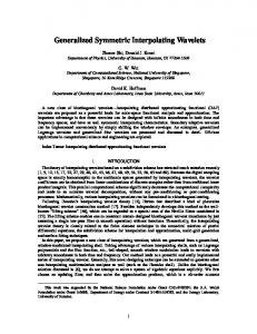
50
Figure 1: Plot of the motorcycle impact data together with the wavelet regression estimates g^ based on the Daubechies scaling function with lter of order 8 for J = 3 (dotted line), J = 4 (solid line) and J = 5 (dashed line). Cross validation selected the curve J = 4 as giving the best t. The wavelet estimator (10) has the advantage that the optimal asymptotic rates of mean square convergence hold for weaker conditions on the underlying function g (g 2 B22s for s > 1=2) than must be assumed in obtaining similar results for other types of smoothing. A disadvantage is that one can derive an asymptotic normality of the estimator 10
at dyadic points only. At non-dyadic points, the asymptotic variance of the estimator, while remaining bounded, oscillates and asymptotic normality cannot be obtained. This phenomenon of erratic oscillations in the variance was also observed by Hall & Patil [48]. Figure 1 displays the motor-cycle impact data given in Hardle [51]. The observations consist of accelerometer readings taken through time in an experiment on the e�cacy of crash helmets. For several reasons the time points are not regularly spaced. The cascade algorithm described in subsection 2.3 of Section 2 was used to compute the weights de ning the estimator. The computational complexity of the algorithm for a general design is of the order O(n2 ) and does not really take advantage of the fast discrete wavelet transform. To obtain a faster computational algorithm in the xed design model with equidistant nonrandom design points ti within [0; 1], Antoniadis [7] used another linear method that takes advantage of the DWT transform. Assuming that g is a function [s]-times continuously di�erentiable in R , and such that its [s]th derivative satis es a Lipschitz condition of order s ? [s], when s > 1 and s 62 N , or that g is a function s ? 1 times continuously di�erentiable in R , and such that its (s ? 1)th derivative satis es a Lipschitz condition of order 1 when s 2 N , and taking the design points to be of the form ti = i�, with � = 2?N for i = 0, : : : , n ? 1, where n = 2N , he obtains a linear wavelet estimator that attains again the optimal asymptotic mean squared error rates and that is asymptotically normal at dyadic points. The approach is as follows. One advantage of the nested structure of a multiresolution analysis is that it leads to an e�cient tree-structured algorithm for the decomposition of functions in Vn for which the coe�cients < g; 'n;k > are given. However, when a function is given in sampled form there is no general method for deriving the coe�cients < g; 'n;k >. A rst step towards the curve estimation method is to approximate the projection PVn by some operator �n in terms of the sampled values g( 2kN ) and to then derive a reasonable estimator of the approximation �n g. Using coi ets (see Daubechies [27]) that have L vanishing moments with L > [s], such an estimator of �ng is obtained by N ?1 2X X ? N= 2 ? N= 2 b g^n(t) = �ng(t) = 2 Yk �n;k(t) = 2 Yk �n;k (t)
k2Z
k=0
where the use of coi ets (wavelets for which the scaling function has integral 1 but admits zero moments) allows to approximate the coe�cients < g; �n;k > by 2?N=2g( 2kN ) with an error O(2?N=2 2?ns). In order to smooth correctly the data, to each each sample size n = 2N one then associates a resolution j (n) = log2 (n)=(1 + 2[s]), and estimates the unknown function g by the orthogonal projection of g^n onto Vj(n). Once again the parameter j (n) governs the smoothness of the estimator. Another class of linear wavelet estimators that used in literature is derived within the framework of regularization methods. Such estimators appear in Devore & Lucier [30], 11
in a 1993 technical report of Antoniadis recently publised ([5]) and in Amato & Vuza [2]. In smoothing splines, a popular method for nonparametric regression problems such as the ones treated here a � th order smoothing spline g�(x) is de ned to be that function with square integrable � th derivative which minimizes over the Sobolev space H � [0; 1] the \discrete" functional: Z 1� ?1 � 1 nX 2 (� ) (t) 2 dt; g ( Y i ? g (ti)) + � n i=0 0 where g(��) indicates �2 the � th derivative of g (see for example Wahba [86]). The \curvature" R 1 ( � ) term 0 g (t) dt is a penalty term for lack of smoothness. Noting that the details of the wavelet coe�cients of a function g at high resolution levels correspond to rough parts of the function, this problem can be generalized by seeking at the minimizer of an expression similar to p (P f ) k�b ng ? f k2L ([0;1]) + �Jspp VJ 2
0
(11)
where J0 is a coarse resolution level, �b ng is the interpolation estimate based on coi ets and Jspp is the equivalent norm of the Besov space Bpp2 ([0; 1]). In Antoniadis [5] as well as in Amato & Vuza [2] the particular choice p = 2 is made. This choice and the use of wavelet decompositions of f and g, allows one to nd an optimal solution to the variational problem given in (11). This is possible because the norms kf k2L2([0;1]) and Js222(f ) can be determined simultaneously by examining the wavelet coe�cients of f and g. The solution to the variational problem is the function
g� =
0 ?1 2JX
k=0
cj0;k 'J0;k +
j ?1 n 2X X ^j;k
j =J0 k=0
j;k ;
(12)
where cj0 ;k ; k = 0; : : : ; 2J0 ? 1 denote the empirical scaling coe�cients of the discrete wavelet transform of the data vector Y and ^j;k = 1 +d�j;k22sj ; j � j0 ; k = 0; : : : ; 2j ? 1 with dj;k being the empirical wavelet coe�cients of Wn;J0 Y. The estimator g� appears as a tapered wavelet series estimator of the regression function, i.e. g� may be viewed as the result of passing the \raw" wavelet series estimate �b ng through a low pass lter controlled by the parameters �s. It can be shown that, asymptotically as n ! 1, if s > 1=2 � ?2s=�(2and s +1) then the mean squared error of the estimate g� behaves like and� if � = O� n O n?2s=(2s+1) : For the practical application of the method, it is of course necessary to have an objective rule for the choice of the \coarse" resolution J0 and the penalty parameter �. As done for previous estimates the resolution level J0 is chosen as log2 n=(2s + 1). Noting that the 12
only term involving � in the upper bound of the risk of the estimator g� is the expectation of k�ng ? g�k2L2 ([0;1]), the data-driven determination of � is based on minimization of an appropriate estimate of this expectation and the knowledge of the noise variance �2 . A possible choice for an estimate of the noise variance is the one suggested by Muller [64]: nX ?1 2 2 �^ = 3(n ? 2) [Yi ? 12 (Yi?1 + Yi+1)]2; i=2 obtained by tting constants to successive triples of the data. Lemma 1 of Muller shows �^ 2 is almost surely consistent and � (log n) 21 +� � 2 2 j�^ ? � j = O n 12 a.s. as n ! 1 for any � > 0. In spline smoothing, another method for providing, via a further approximation, an objective estimate for the minimizers of the integrated mean squared error of the estimates is generalized cross-validation. It is easy to see that the wavelet estimator introduced by regularization appears as a particular diagonal linear shrinker (see Donoho and Johnstone [33]). For each resolution j � J0, the wavelet coe�cients dj;k are shrinked by a factor 1=(1 + �22sj ) which is level dependent. Assuming that g is a periodic function, Amato & Vuza [2] use J0 = 0 and choose � as the minimizer of the \GCV" function 2 Vn(�) = h k1(In ? Rn(�))Yk i2 n?1 Tr(In ? Rn (�)) where Rn (�) denotes this diagonal shrinkage operator. The linear estimate suggested by Devore and Lucier [30] approximately minimizes the penalized functional (11) by a factor of 2 and is obtained by projecting the data vector on VK where K is chosen such that kgk2B22s 22n !1=(s+1) 2 K : 2 = �2 While a reasonable estimate of the unknown variance can be obtained, it seems more di�cult to estimate the norm kgk2B22s unless one has a precise upper bound for this norm. To end this subsection, we brie y mention an interesting result of Donoho [32] where a linear wavelet estimator for an equidistant regression model with independent Gaussian errors is shown to attain the best asymptotic minimax rate (n?1 log n) =(2 +1) in the supnorm for the class of functions m m ff : sup jf (jxx)??yfj� (y)j � Lg \ ff : sup jf (x)j � B g; x;y2[0;1]
x2[0;1]
for L > 0, B > 0 and 1=2 < = m + � with 0 < � � 1. A more elementary and transparent proof of his result is also given in the paper of Oudshoorn [71]. This result is interesting because it shows that with linear wavelet estimators one can attain minimimax rates for sup-norm loss. 13
3.2 Nonparametric density estimation The estimation of probability density functions from data is another example of basic problems in applied statistics. The idea to use a wavelet series expansion for the estimation of probability functions was rst considered by Doukhan and L�eon [40], Antoniadis and Carmona [6], Kerkyacharian and Picard [56] and Walter [87]. These works are motivated by the multiresolution decomposition associated with wavelet orthonormal bases and the localized character of wavelet expansions. Specialized versions of histograms constructed via Haar basis decompositions are described in Chapter 12 of Walter [88] and some interesting properties of such Haar-based estimators on the interval [0; 1] are discussed in Engel [41]. All these papers assume i.i.d. observations. In Antoniadis and Carmona [6], the unknown density belongs to the Sobolev space B22s , s > 0, whereas in Kerkyacharian and Picard [56] f belongs to the Besov space Bpps , p � 1, s > 0. The consistency rates obtained by these authors for linear wavelet estimators are respectively E kf ? f^n k22 = O (n?2s=(2s+1) ) and
kf ? f^nkpp = O(n?ps=(2s+1) ): A precise asymptotic expression for E kf ? f^nk22 in the case of f 2 B22s , s > 0 was given E
later by Masry [60] for more general stationary processes. In the i.i.d. case the asymptotic expression is shown to be exactly of the form n?2s=(2s+1) E kf ? f^nk22 ! 1 as n ! 1. With the basic introduction of wavelets in Section 2 we can examine more closely the way these estimators are constructed. Let X1; X2; : : : ; Xn be an i.i.d. sample and let f be the probability density of X1 which is assumed to exist and satisfy f 2 L2 (R ). Using an orthonormal wavelet basis, the wavelet representation of f is then given by
f=
X
cJ0;k 'J0;k +
k2Z
1 X X
dj;k
j =J0 k2Z
j;k ;
where J0 represents again a coarse level of approximation. The rst issue in estimating f involves in estimating the coe�cients in the above decomposition. This can be accomplished by using their empirical counterparts, that is
c^J0 ;k and
X = n?1 ' n
i=1
X d^j;k = n?1 n
i=1
14
J0 ;k (Xi );
(13)
j;k (Xi ):
(14)
Given these estimates, one then estimates f by
X XX^ dj;k f^n = c^J0;k 'J0;k + J1
k2Z
j =J0 k2Z
j;k ;
(15)
where J1 � J0 is a resolution suitably chosen. Note that the estimator f^n de ned in (15) belongs to VJ with J = J1 + 1 and can be written as
X f^n = c^J;k 'J;k : k2Z
(16)
For linear wavelet density estimators the smoothing parameter is the index J of the highest level to be considered. Several strategies for the automatic choice of the tuning parameter have been suggested in the literature. Walter [88] discusses an automatic algorithm to choose the most appropriate level J by using the integrated mean square error criterion IMSE =
Z � �2 E f^n (t) ? f (t) dx:
The algorithm begins by computing the c^K;k at a high and non optimal level, estimating the IMSE of the resulting estimate, and then recursively computing lower-level coe�cients and the associated estimated error. The level J chosen by Walter is the one at which the estimated error increases most rapidly when moving from a level to the next coarser. Another method that is considered to be optimal with respect to the IMSE criterion is the one discussed by Tribouley [82]. The choice is based on the cross-validation principle and results in the minimization with respect to J of the expression: CV(J ) =
X" k
2
n X
n(n ? 1) i=1('J;k
(X ))2 ? i
#2 n n + 1 (X 2 n2 (n ? 1) i=1 'J;k (Xi)) :
For densities that are compactly supported within a known interval ]a; b[ and that are continuously di�erentiable, a method for choosing J involving the Fisher functional of the density f , de ned by Z 1 " d #2 F (f ) = f (t) dt f (t) dt R
has been introduced recently by Vannuci and Vidakovic [83]. The \optimal" J is chosen such that the wavelet estimator f^n has an estimated Fisher information close to the theoretical minimal bound 4�2=(b ? a)2 .
15
J=1
J=2
0.8
0.8
0.6
0.6
0.4
0.4
0.2
0.2
0
0
-0.2
0
2
4
-0.2
6
0
2
J=3 0.8
0.6
0.6
0.4
0.4
0.2
0.2
0
0
0
2
6
4
6
J=4
0.8
-0.2
4
4
-0.2
6
0
2
Figure 2: Linear wavelet-based density estimates for the duration times of eruption from the Old Faithfull geyser data set using Daubechies lters of order 5 and four choices of J . Figure 2 displays smooth wavelet-based density estimates of the duration times of eruption from the Old Faithfull geyser in Yellowstone National Park. The Old Faithfull data set has been often used as a benchmark for density estimators. The above \linear" method of viewing wavelet-based density estimators might not be seen so much as an alternative to the kernel approach but as a way of enhancing that technique. Indeed, the wavelet estimators described above are nothing else than generalized kernel estimators based on kernels of the form EJ . The resolution J permits a global level of smoothing in terms of the frequency of the scaling function and 2?J is analogous to bandwidth for a kernel estimator. However, contrary to the case of classical kernel estimators, the terms representing bias and variance of wavelet-based density estimators oscillate erratically with a wavelength of the same order as 2?J . Indeed, as proved by Hall & Patil [48], the classical pointwise bias and variance formulae, bias(t) = E f^n(t) ? f (t) ' a1(t)2?Js and
variance(t) = varffn(t)g ' a2(t)2J =n for smooth functions a1 and a2 are no longer valid. They are replaced by bias(t) ' a1 (t)a3 (2J t)2?Js 16
and
variance(t) ' a2 (t)a4(2J t)2J =n for new nondegenerate functions a3 and a4. The erratic oscillations represented by a3(2J t) and a4 (2J t) can be clearly observed in the estimates displayed in gure 2. One way to reduce these oscillations, thus resulting in a smaller mean-squared error, is to not insist on choosing a smoothing frequency that is a power of 2 for the wavelet estimator. Hall & Patil [48], suggest using the family of orthonormal scaling functions �k (x) = p1=2 '(px + k) where p > 0 denotes an arbitrary positive number. It is easy to see that when p = 2J one has �k = 'J;k . This generalization permits a wider range of choices for the smoothing parameter in applications of curve estimation. A quanti cation of the advantages of noninteger resolution levels as well as some techniques for choosing the smoothing parameter by cross-validation as is done for kernel estimation is given in Hall & Nason [47]. When p = p2j the resulting estimator may be seen as a classical wavelet-based estimator applied to a preliminary binned data with binwidth proportional to p (see Antoniadis & Pham [8]). This is also the approach taken by by Antoniadis, Gr�egoire and Vial [10], to generalize the fast linear wavelet estimators to general design nonparametric regression and density estimation. There is a potential problem in using wavelets for density estimation. When using general scaling functions there is no guarantee that the estimates are positive or integrate to 1. Indeed, it does happens that they are often negative in the tails of the distribution. Moreover there is no easy way to norm the wavelet estimator, except to numerically integrate the estimate in order to work out the norming constant. Walter [88] considers estimating the density function indirectly, by using wavelets to estimate the Fourier transform of the density, and then transforming back but he points out that the rate of convergence of such an estimate may be relatively slow. Another approach used in the literature, that will be discussed further when nonlinear wavelet estimation methods will be presented, is to estimate the square root of the density and square back the estimate after. The idea of the above transformation can be found & Gaskins [46]R p in the context of penalized likelihood methods. The condition p RinfGood 1 = 2 (x)dx = 1 becomes ( f (x)) dx = 1, so that f 2 L2. Pinheiro and Vidakovic [73] do exploit this idea of estimating the square root of the density in a wavelet setting, but, in order to get estimators of the needed wavelet coe�cients they use a rough but consistent pre-estimator of the unknown density. There is no theoretical or convincing numerical evidence in their paper that optimal asymptotic rates can be obtained in this way.
17
Hall & Patil 0.6 0.5 0.4 0.3 0.2 0.1 0
0.5
1
1.5
2
2.5
3
3.5
4
4.5
5
5.5
3.5
4
4.5
5
5.5
Binning 0.6 0.5 0.4 0.3 0.2 0.1 0
0.5
1
1.5
2
2.5
3
Figure 3: Linear wavelet-based density estimates for the duration times of eruption from the Old Faithfull geyser data set using Hall and Patil's scaling functions (left) and Antoniadis et al.'s pre-binning (64 bins), both based on Daubechies wavelet lters of order 4 adapted to the interval. Figure 3 displays the linear estimates corresponding to the Hall & Patil approach as well as on the binning + smoothing approach of Antoniadis et al. To avoid negative values of the estimates Pinheiro and Vidakovic's [73] idea was used. Along the same lines, but using a di�erent approach and di�erent estimators, is the research completed by Penev & Dechevsky [72]. Since their method deals principally with nonlinear thresholding methods, it will be discussed in the next Section.
4 Nonlinear wavelet methods for curve estimation In the previous section the nonparametric estimation of regression functions and probability density functions has been restricted to the context of linear wavelet-based estimators. The application of these methods has provided only asymptotic upper bounds to the integrated squared error for functions that are traditionally smooth. For functions that might not be smooth in the classical sense, nonlinear wavelet-based estimation methods provide levels of smoothing which automatically adapt to local variations of roughness of 18
the curve. Nonlinear wavelets methods in statistics were introduced by Donoho and Johnstone [33], [34], [36] and Donoho, Johnstone, Kerkyacharian and Picard [37], to cite only few of their papers. They permit two non-overlapping levels of smoothing, one global, via the frequency of the scaling function, and the other one local, via the scale of the wavelet function. This section deals with the ability of the nonlinear component of wavelet methods to adapt to local features of an unknown curve, and thus to correct for more erratic features of the curve no taken into account by the linear component.
4.1 Nonparametric regression In this subsection, contrary to the assumptions used in the linear case, we restrict our attention to nonparametric regression models on the unit interval with an equidistant deterministic design and a Gaussian noise. Possible extensions that might be possible for a random design and other types of noise will be discussed later. The paper by Donoho, Johnstone, Kerkyacharian and Picard [37] is perhaps the most signi cant paper from both a mathematical and practical point of view for the existence of nonparametric function estimators that behave in a (near) asymptotic optimal way simultaneously for a broad range of function spaces (Besov or Triebel spaces) not considered before in statistics and a variety of loss measures (Lp-losses) and whose de nitions are independent of the set of function spaces considered. Mathematically it gives a uni ed treatment of optimal rates of convergence for nonparametric function estimation in a very general setup. This is achieved by using the approximating properties of wavelet bases and the close relation between the problem of minimax estimation and the theory of optimal recovery, a survey of which can be found in a paper by Michelli and Rivlin [63]. The connection with deterministic optimal recovery problems is obtained by means of a simple but powerful thresholding device on the empirical wavelet coe�cients, which works reasonably well in practice. We refer the reader to the above papers for the exact assumptions and consistency rates, which are nearly optimal in the sense that they are equal to the optimal asymptotic rates up to a log n multiplicative factor. Let us now further describe the regression model and the methods of estimation. The data are discrete and follow the xed equidistant design regression model on [0; 1]:
Yi = f (ti) + ��i ; i = 1; : : : ; n = 2N ; where ti = i=n, and the �i's, the noise in the observations, are i.i.d. N (0; 1) random errors. To this data set, we apply the discrete wavelet transform Wn;J0 : R n ! R n for some J0 < N and for simplicity of exposition we will use a periodic version of the transform. Heuristically, the assumption made in the various papers cited above is that
Z
2N=2 '((t ? i=2N )2N )f (t) dt ' f (i=2N )=2N=2 ; R
19
if N is large. Such an assumption is reasonable when the function f is su�ciently smooth (see Section 3) but the approximation seems questionable when f belongs to classes of functions that may be not even continuous. To overcome this, one may think of the 2?N=2Yi's as noisy versions of the left hand side of the above formula. Let c = 2?N=2 Wn;J0 Y be the empirical scaling coe�cients, let = 2?N=2 Wn;J0 f and let z = 2?N=2Wn;J0 �. Since the transformation is linear one has, for j = 0; : : : ; N ? 1 and k = 0; : : : ; 2j ? 1:
cj;k = j;k + 2?N=2 �zj;k ;
(17)
and since it is orthonormal, the zj;k are i.i.d. N (0; 1). The respective mean squared errors in estimating the wavelet coe�cients of f or f are therefore the same. Now, for the large classes of functions considered, and with the use of su�ciently regular wavelets the vector is generally sparse, i.e., relatively few components are large. The noise in the original sequence Yi is spread out uniformly among all empirical wavelet coe�cients. The heuristic idea underlying the Donoho-Johnstone procedure is to choose the set of coe�cients that contain signi cant signal and to remove the noise component from the noisy coe�cients. This is achieved by thresholding. The thresholding estimator of the true coe�cient j;k , j � J0 is de ned by
^j;k = p�n ��
pnc ! �
j;k
(18)
where the function �� in (18) is either the hard thresholding function
8 < ��H (x) = : x; if jxj > �; 0; otherwise:
(19)
or the soft thresholding function
8 > < x ? �; if jxj > �; S �� (x) = > 0; if jxj � �; : x + �; if x < ?�:
(20)
T Once the thresholding is performed, one applies the inverse empirical transform Wn;J 0 to the estimated thresholded vector, obtaining the estimated regression curve f^n (t). The method is therefore simple and practical, with an algorithm that functions in order O(n) operations. The above arguments produce the regression estimator X XX^ j;k j;k : f^n = cJ0;k 'J0;k + j �J0 k
k
The rst part of the right hand side is identical to the linear wavelet-based estimator studied in the previous Section. The second part enhances the linear estimator by incorporating through thresholding some wavelet terms. 20
Clearly, when using either type of wavelet thresholding, the choice of the cut-o� resolution J0 and of a threshold � is a fundamental issue (see gure 4). The typicalpsparsity of the j;k sequence ensures that most of the appropriately scaled coe�cients ncj;k=� are essentially white noise. Motivated frompthe \large deviation" nature of the problem, Donoho and Johnstone suggest taking � = 2 log n, named universal threshold. The procedure is proven to be asymptotically optimal for many classes of functions and makes no a priori assumptions on the particular class that f may belong, producing therefore an asymptotically adaptive estimator. Threshold = 1.7
Threshold = 0.5
•
•
0
• • • • • • •• •• • • • • • •• • • • • • •• • • • •
2 -3
-2
• • •• • •• • • • • • • • • • • •
0.2
••• • •• • ••
• • • • • • ••• • • • • • • •• • • • • •• • • • •
• •• • •
-1
• •• • •
0.0
•• • • •• •
1
1
••• • •• • ••
-1 -2 -3
• • • • •• •••• • •• • • • • •• • • •• •• • • • •• • • • • • •• •• • • • • • • •• • • • • • ••• • • • •
0
2
•• • • •• •
0.4
0.6
0.8
1.0
• • • • •• •••• • •• • • • • •• • •• •• • • • •• • • • • • •• •• • • • • • • •• • • • • • ••• • • • • •
•
• • •• • •• • •• • • • • • • • • 0.0
0.2
0.4
0.6
0.8
1.0
Figure 4: The e�ect of varying the threshold value on the resulting wavelet estimator from a simulated data set. Another method for global thresholding proposed by Donoho and Johnstone [33] is labeled minimax thresholding. Brie y, the performances of shrinkage estimators are compared to the benchmark
X Bn(�; �2) = �2 + min(�i ; �2) i=1 m
where, to simplify the notation, � denotes the m-dimensional vector of wavelet coe�cients, which are observed with a white noise of variance �2. The above benchmark is derived by using the fact that if one has knowledge of the true coe�cients, an ideal minimal meansquared error estimator is obtained by setting a noisy coe�cient to zero if the variance �2 of the noise is larger than the square of the true wavelet coe�cient. Note that the benchmark Bn(�; �2) is small in comparison to m�2 (the total variance in the signal observed with noise) if � is sparse, and usually serves as a measure for the sparsity of �. One of the most signi cant results of Donoho and Johnstone is that, in the case one observes a realization from a Gaussian vector m-dimensional vector U � Nm(�; �2Im), the following upper bound holds supm R
�2
E
k��Sn (U) ? �k2 � (1 + 2 log n); Bn(�; �2)
21
p
when �n = 2 log n is taken to be the universal threshold. It is also proven that the 2 log n factor cannot be improved, that is 1 inf sup E k��S (U) ? �k2 � 1: lim infn!1 2 log n � � Bn(�; �2) In his thesis, Gao [43], proves similar results for i.i.d. variables with exponential tails. Recently, Averkamp and Houdr�e [14], obtained a stronger result of this type for a wider class of distributions. Using the above, when � is the vector of wavelet coe�cients of the regression function, the the minimax thresholded wavelet estimator is obtained by computing the threshold ��n that attains the bound E k��S (U) ? � k2 inf sup � � Bn(�; �2) : Note however that the above results cannot be applied to the empirical coe�cients of a regression with non-normal errors since then the noise in the wavelet coe�cients is no longer independent nor identically distributed. For some particular non-Gaussian regression models a possible approach, using some large deviation results, is one proposed by Neumann and Spokoiny [69], where a risk equivalence between some non-Gaussian regression models and Gaussian white noise models is established. The threshold ��n does not exist in analytical form but a numerical approximation for a range of sample sizes are given in Donoho and Johnstone [33]. For a given sample size, the optimal minimax threshold is typically smaller than the universal one, and thus results in less smoothing (see gure 5). Minimax thresholding
Universal thresholding
•
2
•• • • •• •
1
•••
0
• •• • ••
-3
-2
-1
••
• • • • • • • • • ••• • • • • •• • • • •• • • • • •
• • • • •• •••• • •• • • • • •• • • •• •• • • • •• • • • • • • •• •• • • • • • • •• • • • • • ••• • • • •
• ••
• • •• • •• • • • • • • • • • • •
0.0
0.2
0.4
0.6
0.8
1.0
• •• • • • • • • •••••• • •• •• ••• •• • • •• • • • • • • • •• ••• •• • • • • •••• • • • • • •• •• • • • •• • • • •• • • •• •• • • • • • • • • •••• • •• •• • • • • • • ••• • •• ••• •• • • • • • ••• • • • •• • • • • •
0.0
0.2
0.4
0.6
0.8
1.0
Figure 5: Minimax and universal thresholding applied to the simulated data set in gure 4. Both thresholding rules require an estimate of the usually unknown variance �2. When it is known that the underlying regression function is Holder continuous an estimator as the one described in Section 3 can be used. Donoho and Johnstone [33] propose a robust estimate of � by taking the median absolute deviation of the coe�cients at the nest level of the empirical decomposition median(jcN ?1;k )j) �^ = median(jcN ?1;k0? :6745 22
since typically there is also some signal present even at the nest level. The estimators described above, while applicable to a wide range of variable frequency curves, usually provide an excessive amount of smoothing when applied to curves that are piecewise smooth. Their mean-squared errors are asymptotically dominated by bias. To address this problem, Donoho and Johnstone [35] look at a variant with level-dependent thresholds. The method, called Sureshrink employs an unbiased risk estimation that is due to Stein [78] and is shown in Ogden [70] to be in relation with Akaike's information criterion (AIC), introduced by Akaike for times series modeling. Hall and Patil ([48], [49], [50]) studied asymptotic wavelet shrinkage methods in nonparametric curve estimation from the di�erent viewpoint of a xed target function, as opposed to the minimax approach of Donoho et al.. In the case of functions that are smooth or piecewise smooth in the classical sense, using wavelet decompositions which allow non-integer resolution levels, already described in Section 3, they derive necessary and su�cient conditions on the asymptotic form of the threshold and smoothing parameters for their resulting curve estimator to achieve optimal mean square convergence rates. Most of the methods and results described above are asymptotic in character. As with any asymptotic result, there remain doubts as to how well the asymptotics describe small sample behavior. These issues are addressed by Marron et al. [59] using the tools of exact risk analysis, which was developed in Gasser and Muller [45], and rst applied to wavelet estimators by Antoniadis et al. [7]. Finite sample performance of thresholded wavelet estimators has also been studied by Bruce and Gao [19], where computationally e�cient formulas for computing the exact pointwise bias, variance and L2 risk of thresholded wavelet estimators in nite sample situations are derived, thus complementing the tools of simulation and asymptotic analysis. Comparing hard and soft shrinkage, hard shrink tends to have bigger variance (because of the discontinuity of the shrinkage function) and soft shrink tends to have bigger bias (because of shrinking all big coe�cients towards 0 by �). To remedy these drawbacks, and paralleling the choice of shrinkage functions with that of in uence functions in robust statistics, Bruce and Gao [20] introduce a general semisoft shrinkage function
8 > if jxj � �1 sgn(x) �2 ?�1 if �1 < jxj � �2 :x if jxj > �2 ;
that o�ers some advantages over both hard shrinkage (uniformly smaller risk and less sensitivity to small perturbations in the data) and soft shrinkage (smaller bias and smaller overall L2 risk). A drawback of this semisoft rule is that it requires two thresholds, thus making threshold selection problems much harder and computationally more expensive for adaptive threshold selection. 23
One way to choose the thresholds is by generalized cross-validation proposed rst for nonlinear wavelet series estimators by Weyrich and Warhola [91]. Recently, Jansen et al. [53] have shown that, under appropriate conditions, this generalized cross-validation choice is asymptotically optimal, in the sense of yielding asymptotically the threshold that minimizes the expected mean squared error. Other data-driven methods for the choice of the smoothing parameter(s) in thresholding wavelet estimators have also been proposed in the literature. For a detailed account and description of these methods the reader is referred to the papers by Nason ([66], [65]) or the book by Ogden [70].
4.2 Density estimation Nonlinear wavelet-based density estimators in the i.i.d. setting were introduced by Johnstone et al. [54] and Donoho et al. [38] and parallel exactly the results obtained for the regression case, although the proofs are entirely di�erent. For the appropriate compactly supported wavelet basis, they take the form
X XX ^ f^n = c^J0;k 'J0;k + ��j (dj;k) J1
k2Z
j =J0 k2Z
j;k ;
(21)
with properly chosen resolutions J0, J1 and level dependent thresholds �j . As pointed earlier, the estimator (21) may be seen as a coarse approximation of f at level J0 plus some details q that are added to improve the approximation. Using J1 = log2 n ? log2(log n), �j = A (j ? J0)=n, where A is some constant and J0 is chosen according to the regularity of � and the sample size, the thresholded estimator f^n in the papers cited above (see also Delyon and Judistsky [29]) is shown to be asymptotical optimal in the sense that, for s > 1=p and p � (1 + 2s)p, it attains the minimax Lp rate 0
0
! log n (s?1=p+1=p )=(1+2(s?1=p)) n 0
in the class of densities in the Besov space Bpqs with Jspq (f ) � M , where M is a given constant. This rate cannot be attained with linear methods. Note, however, that when p ! 1, Masry [61] has shown that this rate is attained by linear estimators and thus nonlinear estimators do not improve the rate of convergence in this case. We have already mentioned the approach taken by Penev and Dechevsky [72], to estimate rst by wavelet methods the square root of the density before taking its square as the nal estimate, in order to preserve the non-negativity while still retaining the asymptotic minimax properties. The nonlinearity of the estimates is justi ed by the fact that they assume that it is the square root of f that belongs to a Besov ball. However, they prove that there are some reasonable connections between Besov regularity of f and 0
24
p
that of f . The advantage of the estimate they propose is that it can be normed to integrate to 1 very easily without numerical integration. Some data dependent methods for choosing J0 (Tribouley [82]) and �j have been proposed by Pinheiro and Vidakovic [73] and more recently by Vannucci and Vidakovic [83].
5 Related topics The regression models discussed in the previous sections involve additive white noise of constant level, no weighting and most of the time normality. Antoniadis and Lavergne [9] extend the linear wavelet-based methods to data with heteroscedastic noise. More recently, an extension of Donoho and Johnstone's wavelet shrinkage smoothing technique to handle data with heteroscedastic noise has been given by Gao [44]. Johnstone and Silverman [55] have considered the extension to more general noise models than the white noise model. When the noise is stationary, using appropriately chosen level dependent thresholds, they obtain asymptotic minimax results similar to the ones obtained for the white noise regression model. A simpler proof of the optimality of their thresholding procedure is given by Amato and Vuza [3]. Brillinger ([16], [17]) also presents some inferential aspects of the wavelet technique far a deterministic signal in the presence of additive stationary non necessarily Gaussian noise. Function estimation for nonparametric regression with long-range dependence errors is studied in Wang [90]. Wavelet versions of estimators of a hazard rate function in the context of inference for a counting process multiplicative intensity model have been studied by Antoniadis et al. [7]. See also Antoniadis, Gr�egoire and Nason [12] for a contribution to the methodology available for estimating the density and the hazard rate from randomly censored data. The problem of estimating the log spectrum of a stationary Gaussian time series by wavelet thresholding techniques has been addressed by Gao [43] in his thesis. More generally Neumann [68] applied the thresholding procedure in the framework of spectral density estimation for a stationary, possibly non Gaussian time series. It has also been applied by von Sachs and Schneider [85] to the periodogram of a locally stationary process for the estimation of its evolutionary spectrum. A generalization to the problem of recovering f from indirect data Y = K f + �, where K is a known operator has been addressed by Kolaczyk [57] in the context of integration, fractional integration and tomography. Since the basic aim of wavelet analysis is to represent a function as a linear superposition of wavelets centered on a sequence of time points, it forms a natural tool for the investigation of jump points in time varying functions observed with noise. Wavelet methods for detecting and locating the jump points can be found in Vercken and Potier [74], Wang [89] and more recently in Antoniadis and Gijbels [13] and the thesis of Raimondo [75]. 25
Applications of wavelet decompositions in statistical hypothesis testing and model selection appear in particular Fan [42] and Antoniadis et al. [11]. Fan shows that traditional nonparametric tests have low power in detecting ne features such as sharp and short aberrant as well as global features such as high frequency components.These drawbacks are repaired via wavelet thresholding and the Neyman truncation test. Antoniadis et al. [11] discuss how to use wavelet decomposition to select a regression model. Their methodology relies on a minimum description length criterion which is used to determine the number of non-zero coe�cients in the vector of wavelet coe�cients. The developed model selection rule is then applied to testing for no e�ect in nonparametric regression and for martingale structure in time series. To end this section, let us mention some bayesian methods that have been proposed recently for nonparametric curve estimation, since they o�er an interesting and useful alternative to the methods discussed earlier. In Vidakovic [84], the wavelet coe�cients j;k in the decomposition (17) as well as the unknown standard deviation � of the noise are assumed to be independent random variables with an imposed prior distribution. The posterior means of the wavelet coe�cients have the shape of standard soft wavelet thresholding rules and are used to estimate the unknown curve. Other papers considering wavelet shrinkage or thresholding within a Bayesian framework are those by Clyde et al. [22], Chipman et al. [23]. Again, a prior distribution is imposed on wavelet coe�cients of the unknown response function, and the function is estimated by computing the mean of the resulting posterior distribution of wavelet coe�cients. Recent work on this direction has been done by Abramovich et al. [1], with a prior designed to capture the sparseness of the wavelet expansion and a Bayes rule corresponding to the posterior median. Moreover, in the last mentioned paper, the prior model for the underlying regression function is adjusted to give functions falling in any speci c Besov space. In order to achieve this, a relation between the hyperparameters of the prior model and the parameters of the Besov spaces is established.
6 Conclusion So far, we have presented various ways in which univariate orthogonal wavelet series decompositions have been used successfully and realistically in solving theoretical and practical univariate problems of nonparametric statistics. The application of wavelet methods to nonparametric regression has been mostly con ned to the context of the normal distribution, with regularly spaced design points and for problems where both sample size and resolution levels are dyadic. Despite some papers addressing ways to remove these restrictions, some progress on alternative approaches to deal with such problems is very desirable in order to apply wavelet methods \naturally" to the general nonparametric regression setting. 26
A possibility to deal with non-uniform stochastic design would be to apply a discrete wavelet transform for unequally spaced data based on a basis particularly adapted to the irregular grid and constructed via the lifting scheme recently proposed by Sweldens ([80], [79]). Here one entirely abandons the idea of translation and dilation. This gives extra
exibility which can be used to construct wavelets adapted to irregular samples. However, to use such an approach some progress is needed on the deeper mathematical properties of the resulting scaling functions and these \second generation" wavelets. Research is also needed in developing wavelet based methods to carry over likelihoodbased models such as generalized linear models occurring often in practice. Novel bootstrap methods for wavelet-based nonparametric curve estimation, taking advantage of the O(n) computational e�ciency of wavelet decompositions are also highly desirable, since it is known that when the dimension of the unknown parameter exceeds that of the data, most classical (naive) bootstrap methods for assessing the variability of the estimates and constructing con dence sets fail (see Beran [15]). The usual wavelet-based approach can be further enhanced by using wavelet packets, a generalization of wavelet bases (see e.g. Wickerhauser [92]). In wavelet packet analysis, a function g is represented as a sum of orthogonal wavelet packet functions Wj;b;k at di�erent scales j , oscillations b and location k. By contrast with ordinary wavelet decompositions, in wavelet packet methods, a signal may be represented by many di�erent combinations of wavelet packets. Thus, wavelet packets o�er an enormous amount of exibility in possible sets of basis functions. Adaptative ways to select the most appropriate set of basis functions with which to represent and estimate a density or a regression are particularly important and pose a number of interesting statistical issues. Some results on adaptative model selection using wavelet packets for white noise models already exist (see for example the papers by Donoho and Johnstone [34] and Saito [77]) but their extension to other types of noise are desirable. Many results in higher dimensions are still incomplete. Theoretical advances in higher dimensional signal approximation bounds, regularity, design techniques, would be very useful in answering some questions that arise in the analysis of additive models in nonparametric regression, slice regression and multivariate density estimation. To conclude let us say that there is room for substantial improvement of the current state of the art.
References [1] Abramovich, F., Sapatinas, T. and Silverman, B. W. (1997). Wavelet thresholding via a Bayesian approach. Technical report , University of Bristol, England. 27
[2] Amato, U. and Vuza, D. T. (1994). Wavelet Regularization for Smoothing Data. Technical report N. 108/94, Instituto per Applicazioni della Matematica, Napoli. [3] Amato, U. and Vuza, D. T. (1996). An Alternate Proof of a Result of Johnstone and Silverman concerning Wavelet Thresholding Estimators for Data with Correlated Noise. Revue Roumaine Math. Pures Appl. 41, 431{438. [4] Antoniadis, A. (1994). Smoothing noisy data with coi ets. Statistica Sinica 4(2), 651{678. [5] Antoniadis, A. (1994). Smoothing noisy data with tapered coi ets series. Scand. Journal. of Statistics 23, 313{330. [6] Antoniadis, A. and Carmona, R. (1991). Multiresolution analyses and wavelets for density estimation. Technical report, University of California, Irvine. [7] Antoniadis, A., Gr�egoire, G. and McKeague, I. (1994). Wavelet methods for curve estimation. J. Amer. Statist. Assoc. 89(428), 1340{1353. [8] Antoniadis, A. and Pham, D. T. (1995). Wavelet regression for random or irregular design. Technical report. University of Grenoble. [9] Antoniadis, A. and Lavergne, C. (1995). Variance function estimation in regression with wavelet methods. In A. Antoniadis and G. Oppenheim (eds.), Wavelets and Statistics , Lecture Notes in Statistics, 103, Springer-Verlag. [10] Antoniadis, A., Gr�egoire, G. and Vial, P. (1997a). Random design wavelet curve smoothing. Statistics and Prob. Letters.. In press. [11] Antoniadis, A., Gijbels, I. and Gr�egoire, G. (1997b). Model selection using wavelet decomposition and applications. Biometrika. To appear. [12] Antoniadis, A., Gr�egoire, G. and Nason, G. (1997c). Density and hazard rate estimation for right censored data using wavelet methods. Technical report. University of Grenoble. [13] Antoniadis, A. and Gijbels, I. (1997). Detecting abrupt changes by wavelet methods. Technical report. University of Grenoble. [14] Averkamp, R. and Houdr�e, C. (1996). Wavelet thresholding for non (necessarily) Gaussian noise: a preliminary report. Technical report, Georgia Institute of Technology, Atlanta. [15] Beran, R. (1994). Bootstrap variable selection and con dence sets. Technical report, University of California, Berkeley. 28
[16] Brillinger, D. R. (1994). Some River Wavelets. Environmetrics 5, 211{220. [17] Brillinger, D. R. (1995). Some uses of Cumulants in Wavelet Analysis. J. Nonparam. Statistics 4. [18] Bruce, A. G. and Gao, H.-Y. (1994). S+Wavelets, Users manual. StatSci, Seatle. [19] Bruce, A. G. and Gao, H.-Y. (1996). Understanding WaveShrink: Variance and bias estimation. Biometrika 83 (4), 727{746. [20] Bruce, A. G. and Gao, H.-Y. (1997). WaveShrink with rm shrinkage. Statistica Sinica , to appear. [21] Buckheit, J. B. and Donoho, D. (1995). Wavelab and Reproducible research. In A. Antoniadis and G. Oppenheim (eds.), Wavelets and Statistics , Lecture Notes in Statistics, 103, Springer-Verlag. [22] Clyde, M., Parmigiani, G. and Vidakovic, B. (1995). Multiple shrinkage and subset selection in wavelets. Technical report DP 95-37, Duke University. [23] Chipman, H. A., Kolaczyk, E. D. and McCulloch, R. E. (1995). Adaptative Bayesian Wavelet Shrinkage. Technical report , University of Chicago. [24] Chui, K. (1992). Wavelets: A Tutorial in Theory and Applications. Academic Press, Boston. [25] Cohen, A., Daubechies, I. and Vial, P. (1993). Wavelets on the interval and fast wavelet transforms. Applied and Comp. Harmonic Analysis 1(1), 54{81. [26] Cohen, A. and Ryan, R. D (1995). Wavelets and Multiscale Signal Processing. Chapman & Hall, London. [27] Daubechies, I. (1992). Ten Lectures on Wavelets . CBMS-NSF regional conferences series in applied mathematics. SIAM, Philadelphia. [28] Daubechies, I. D. and Lagarias, J. C. (1991). Two-scale di�erence equations: Existence and global regularity of solutions. SIAM Journal on Math. Analysis. 22, 1388{1410. [29] Delyon, B. and Juditsky, A. (1996). On minimax wavelet estimators. Applied and Comp. Harmonic Analysis 3, 215{228. [30] DeVore, R. and Lucier, B. J. (1992). Fast wavelet techniques for near-optimal signal processing. In IEEE Military Communication Conference , pp. 1129{1135. 29
[31] DeVore, R. , Jawerth, B. and Popov, V. (1988). Interpolation of Besov spaces. Trans. Amer. Math. Soc. 305, 397{414. [32] Donoho, D. (1994). Asymptotic risk for sup-norm loss: solution via optimal recovery. Prob. Theory and Related Fields. 99, 145{170. [33] Donoho, D. L. and Johnstone, I. M. (1992). Minimax estimation via wavelet shrinkage. Technical report, Stanford University. [34] Donoho, D. L. and Johnstone, I. M. (1994a). Ideal spatial adaptation by wavelet shrinkage. Biometrika 81, 425{455. [35] Donoho, D. L. and Johnstone, I. M. (1995). Adapting to unknown smoothness via wavelet shrinking. J. Am. Statist. Assoc. 90, 1200{1224. [36] Donoho, D. L. and Johnstone, I. M. (1994b). Ideal denoising in an orthonormal basis chosen from a library of bases. Compt. Rend. Acad. Sci. Paris A 319, 1317{1322. [37] Donoho, D. L., Johnstone, I. M., Kerkyacharian, G. and Picard, D. (1995). Wavelet shrinkage: asymptopia (with discussion)? J. Roy. Statist. Soc., Ser. B 57(2), 301{370. [38] Donoho, D. L., Johnstone, I. M., Kerkyacharian, G. and Picard, D. (1996). Density estimation by wavelet thresholding. Ann. Statist. 24(2), 508{539. [39] Doukhan, P. (1990). Consistency of delta-sequence estimates of a density or of a regression function for a weakly dependent stationary sequence. S�eminaire de Statistique d'Orsay, Universit�e Paris Sud, 1991. [40] Doukhan, P. and L�eon, J. (1990). D�eviation quadratique d'estimateurs de densit�e par projection orthogonale. Compt. Rend. Acad. Sci. Paris A 310, 424{430. [41] Engel, J. (1990). Density estimation with Haar series. Statistics and Probability Letters 9, 111{117. [42] Fan, J. (1996). Test of signi cance based on wavelet thresholding and Neyman's truncation. J. Am. Statist. Assoc. 91, 674{688. [43] Gao, H.-Y. (1993). Wavelet estimation of Spectral denstities in Time series analysis. Ph. D. Thesis, University of California, Berkeley. [44] Gao, H.-Y. (1997). Wavelet Shrinkage Smoothing For Heteroscedastic Data. Technical report, StatSci, Seatle. 30
[45] Gasser, T. and Muller, H. (1979). Kernel estimation of regression functions. In Gasser, T. and Muller, H. (eds), Curve Estimation , Springer-Verlag, Heidelberg. [46] Good, I. J. and Gaskins, R. A. (1971). Density estimation and bump haunting by the penalized maximum likelihood method. J. Am. Statist. Assoc. 75, 42{69. [47] Hall, P. and Nason, G. P. (1996). On choosing a non-integer resolution level when using wavelet methods. Technical report, University of Bristol. [48] Hall, P. and Patil, P. (1995). On wavelet methods for estimating smooth functions. Bernoulli 1, 41{58. [49] Hall, P. and Patil, P. (1996a). E�ect of threshold rules on performance of wavelet-based curve estimators. Statistica Sinica 6, 331{345. [50] Hall, P. and Patil, P. (1996b). On the choice of smoothing parameter, threshold and truncation in nonparametric regression by nonlinear wavelet methods. J. Roy. Statist. Soc., Ser. B 58, 361{377. [51] Hardle, W. (1990). Applied nonparametric regression. Cambridge University Press, Cambridge. [52] Holschneider, M. (1995). Wavelets: An analysis tool. Clarendon Press, Oxford. [53] Jansen, M., Malfait, M. and Bultheel, A. (1997). Generalized crossvalidation for wavelet thresholding. Signal Processing, 56 (1). To appear. [54] Johnstone, I. M., Kerkyacharian, G. and Picard, D. (1992). Estimation d'une densit�e de probabilit�e par m�ethode d'ondelettes. Compt. Rend. Acad. Sci. Paris A 315, 211{216. [55] Johnstone, I. and Silverman, B. W (1997). Wavelet threshold estimators for data with correlated noise. J. Roy. Statist. Soc., Ser. B 59. In press. [56] Kerkyacharian, G. and Picard, D. (1992). Density estimation in Besov Spaces. Statistics and Probability Letters 13, 15{24. [57] Kolaczyk, E. (1994). Wavelet methods for the inversion of some homogeneous linear operators in the presence of noisy data. Ph. D. Thesis, Stanford University. [58] Mallat, S. G. (1989). A theory for multiresolution signal decomposition: the wavelet representation. IEEE Trans. on Pattern Analysis and Machine Intelligence 11, 674{693. 31
[59] Marron, S. J., Adak, S., Johnstone, I., Neumann, M., and Patil, P. (1997). Exact risk analysis of wavelet regression. Journal of Computational and Graphical Statistics . In press. [60] Masry, E. (1994). Probability density estimation from dependent observations using wavelet orthonormal bases. Statistics and Probability Letters 21, 181{194. [61] Masry, E. (1996). Multivariate probability density estimation by wavelet methods: strong consistency and rates for stationary time series. Technical report, University of California, San Diego. [62] Meyer, Y. (1990). Ondelettes et Op�erateurs I: Ondelettes. Hermann, Paris. [63] Michelli, C. A. and Rivlin, T. J. (1975). A survey of optimal recovery. In Michelli, C. A. and Rivlin, T. J. (eds.), Optimal estimation in Approximation theory , pp. 1{54, Plenum, New York. [64] Muller, H. G. (1985). Empirical bandwidth choice for nonparametric kernel regression by means of pilot estimators. Statist. Decisions 2, 193{206. [65] Nason, G. P. (1996). Wavelet regression using cross-validation. J. Roy. Statist. Soc., Ser. B 58, 463{479. [66] Nason, G. J. (1995). Choice of the threshold parameter in wavelet function estimation. In A. Antoniadis and G. Oppenheim (eds.), Wavelets and Statistics , pp. 261{280, Lecture Notes in Statistics, Springer-Verlag, New York. [67] Nason, G. J. and Silverman, B. W. (1994). The discrete wavelet transform in S. Journal of Computational and Graphical Statistics 3, 163{191. [68] Neumann, M. H. (1994). Spectral density estimation via nonlinear wavelet methods for stationary non-Gaussian series. Technical report 99, Institute for applied and stochastic analysis, Berlin. [69] Neumann, M.H. and Spokoiny, V.G. (1993). On the e�ciency of wavelet estimators under arbitrary error distributions. Discussion Paper No. 4, Humboldt Universitat zu Berlin. [70] Ogden, T. R. (1996). Essential wavelets for statistical applications and data analysis. Birkhauser, Basel. [71] Oudshoorn, C. (1994). Wavelet-based nonparametric regression: optimal rate in the sup-norm. Technical report 848, University Utrecht. 32
[72] Penev, S. and Dechevsky, L. (1997). On non-negative wavelet-based estimators. Technical report, University of New South Wales. To appear in J. of Nonparam. Statistics. [73] Pinheiro, A. and Vidakovic, B. (1995). Estimating the square root of a density via compactly supported wavelets. Technical report DP 95-14, Duke University. [74] Potier, C. and Vercken, C. (1994). Spline tting Numerous Noisy Data with discontinuities. In Laurent et al. (eds.), Curves and Surfaces , pp. 477{480, Academic Press, New York. [75] Raimondo, M. (1996). Situations non ergodiques et utilisations de m�ethodes d'ondelettes. Ph. D. Thesis, University Paris 7. [76] Ramlau-Hansen, H. (1983). Smoothing counting processes by means of kernel functions. Ann. Statist. 11, 453{466. [77] Saito, N. (1994). Simultaneous noise suppression and signal compression using a library of orthonormal bases and the minimum description length criterion. In Foufoula-Georgiou, E. and Kumar, P. (eds), Wavelets in Geophysics , Academic Press, New York. [78] Stein, C. (1981). Estimation of the mean of a multivariate normal distribution. Ann. Statist. 10, 1135{1151. [79] Sweldens, W. (1996). The lifting scheme: A custom-design construction of biorthogonal wavelets. Applied and Comp. Harmonic Analysis 3, 186-200. [80] Sweldens, W. (1996). The lifting scheme: A construction of second generation wavelets. Technical report 1995:6, Industrial Mathematics Initiative, Department of Mathematics, University of South Carolina. [81] Triebel, H. (1992). Theory of function spaces II.. Birkhauser, Basel. [82] Tribouley, K. (1995). Practical estimation of multivariate densities using wavelet methods. Statistica Neerlandica 49, 41{62. [83] Vannucci, M. and Vidakovic, B. (1995). Preventing the Dirac disaster: wavelet based density estimation. Technical report DP 95-24, Duke University. [84] Vidakovic, B. (1994). Nonlinear wavelet shrinkage with Bayes rules and Bayes factors. Technical report DP 94-24, Duke University.
33
[85] von Sachs, R. and Schneider, K. (1996). Wavelet smoothing of evolutionary spectra by nonlinear thresholding. Applied and Comp. Harmonic Analysis 3(3), 268{ 282. [86] Wahba, G. (1990). Spline models for observational data . CBMS-NSF regional conferences series in applied mathematics. SIAM, Philadelphia. [87] Walter, G. G. (1992). Approximation of the Delta Function by Wavelets. J. Approx. Theory. 71, 329{343. [88] Walter, G. G. (1994). Wavelets and Other Orthogonal Systems with Applications. CRC Press, Boca Raton, Florida. [89] Wang, Y. (1995). Jump and Sharp Cusp Detection by wavelets. Biometrika 385{397.
82,
[90] Wang, Y. (1996). Function estimation via wavelet shrinkage for long-memory data. Ann. Statist. 24 (2), 466{484. [91] Weyrich, N and Warhola, G. T. (1995). Denoising using wavelets and crossvalidation. In Singh, S. P. (ed), Approximation Theory, wavelets and applications , NATO ASI series C, pp. 523{532. [92] Wickerhauser, M. V. (1994). Adapted Wavelet Analysis: From Theory to Software . AK Peters, Boston.
34