A Space-time Block Code Using Orthogonal Frequency-Shift-Keying Paul Ho
Songhua Zhang, Pooi Yuen Kam
School of Engineering Science, Simon Fraser University, Burnaby B.B. Canada, V5A1S6 E-mail:
[email protected]
ECE Department, National University of Singapore 10 Kent Ridge Crescent, S119260 Singapore E-mail: {engp0975;elekampy}@nus.edu.sg
Abstract—We investigate in this paper an Alamouti-type spacetime block code (STBC) using orthogonal M-ary frequencyshift-keying (MFSK). The signal is coherently detected using the channel estimates derived from the unmodulated (or implicit pilot) component of the orthogonal signal. Exact bit error probability expression for BFSK and tight union bound for MFSK are derived for the proposed coherent ST-FSK receiver. It is observed that the receiver can maintain close to ideal coherent performance even at very fast fading rates. In comparison with differential STBC, the two approaches yield similar error performance in a static fading environment. However, the error performance of differential STBC deteriorates rapidly as the fade rate increases. In terms of implementation complexity and delay, the proposed coherent ST-FSK receiver is similar to differential STBC, as both approaches employ digital filters of similar lengths. The findings in this paper suggest that despite its larger bandwidth requirement, ST-FSK is a very attractive alternative space-time signaling format. Keywords-Frequency-shift-keying (FSK), space time block codes (STBC), implicit pilot symbols.
I.
INTRODUCTION
Recently, transmit diversity has been studied extensively as a method of combating the severe effects of channel fading. Alamouti [1] proposed a simple space-time block code (STBC) using two transmit antennas, which offers both decoding simplicity and full spatial diversity. Later, STBC with orthogonal structure as in [1] was generalized to the case of more than two transmit antennas [2]. However, most the designs of STBC assume perfect channel state information (CSI) at the receiver, which could be difficult to achieve in reality. In one-transmit-antenna systems, noncoherent detection schemes exist which do not require any CSI. Among them, differential encoding and decoding is a popular method that can efficiently detect the signal without any CSI. Analogously, differential STBC (DSTBC) [3]-[5] has been proposed as an alternative to coherent STBC (CSTBC) to achieve diversity gain without channel estimation. It has been shown that conventional differential detection of these schemes has an approximately 3 dB signal energy inefficiency compared to coherent detection in quasi-static fading channel. In a fast fading environment, differential STBC has even worse performance and error floor appears at high signal-to-noise-ratio (SNR). On the other hand, orthogonal M-ary frequency-shift-keying (MFSK) has been shown to be a more stable “noncoherent” detection scheme in fast fading environment [6]. Therefore it is interesting to consider STBC using orthogonal MFSK and compare it with DSTBC. In [7], ST-FSK modulation is introduced in the
context of a unitary ST modulation scheme [8]. However, only conventional noncoherent detection is considered in [7] and its performance comparison with other noncoherent ST modulation such as DSTBC is not addressed. In this paper, we investigate an Alamouti-type STBC utilizing orthogonal MFSK. In light of the alternative interpretation of orthogonal signaling in [6], we develop an effective channel estimation scheme that treats the unmodulated components in adjacent received signal blocks as implicit pilot symbols. The resultant channel estimates are then used to coherently detect the transmitted data symbols. The error performance of this proposed coherent ST-MFSK scheme is analyzed and compared with that of DSTBC. The paper is organized as follows. Section II describes the system model and the channel estimation scheme, where binary FSK (BFSK) is considered first. Section III describes the data detection procedure and the corresponding bit-errorprobability (BEP) analysis. Section IV extends the discussion to M-ary FSK. Section V presents numerical results to demonstrate the performance of our proposed ST-MFSK scheme and compare it with that of DSTBC. Section VI summarizes the paper. II.
SYSTEM DESCRIPTION
A. System Model We first consider an Alamouti-type space-time (ST) block code employing orthogonal binary FSK (BFSK) modulation. Extension to orthogonal MFSK will be provided in Section IV. For the binary case at hand, the basic FSK waveforms are: 1 jπ t wi (t ) = exp (−1)i (1) , i = 1, 2 T T where T is the duration of a subinterval within a ST code interval of TS = 2T . An implicit property of the waveforms in (1) is that they have identical phases at t = nT , n = ...,0,1, 2,...
The received waveforms in the first sub-interval of the kth code interval 2kT < t < (2k + 1)T is r (t ) = c1 [k ]s1 (t ) + c2 [k ]s2 (t ) + n(t ) (2) and in the second subinterval (2k + 1)T < t < (2k + 2)T is r (t ) = −c1 [k ]s2* (t ) + c2 [k ]s1* (t ) + n(t ) , (3) where s1 (t ) and s2 (t ) are data waveforms chosen randomly and independently from the set {w1 (t ), w2 (t )} , and c1 [k ] and c2 [k ] are the fading gains in the two transmission links. These fading gains are assumed constant during one code interval but can vary randomly from one interval to the next according to the Jakes’ fading autocorrelation function.
0-7803-8939-5/05/$20.00 (C) 2005 IEEE
Specifically for a non-selective Rayleigh fading channel, the case of interest in this investigation, the channel gains c1 [k ] and c2 [k ] are independent and identically distributed (iid) complex Gaussian random variables (CGRV) with a mean of zero, a variance of σ c2 = 12 E[| ci (k ) |2 ] , and an autocorrelation function of φ[n] = 12 E ci* [k ]ci [k + n] = σ c2 J 0 ( 2π nf d [2T ]) , (4)
xi [− P ] ci [− P] vi [− P] x [− P + 1] c [− P + 1] v [− P + 1] = i + i Xi = i (11) # # # xi [ P] ci [ P ] vi [ P ] in the neighboring 2 P + 1 code intervals . The optimal filter is [9]
where f d is the maximum Doppler frequency, and J 0 (⋅) is the zero-th order Bessel function. Finally, the additive white Gaussian noise (AWGN) component n( t ) in (2)-(3) has a power spectral density (psd) of N 0 , and the average signalto-noise ratio (SNR) per bit in this paper is defined as kT + T σ2 1 2 γb = E ∫ ci [k ]s (t ) dt = c . (BFSK) (5) N 0 2 N 0 kT The bit error probability (BEP) of our coherent ST-BFSK receiver will be measured against this parameter.
f = φcX Φ XX
B. Channel Estimation Inspired by the new interpretation of orthogonal signaling in [6], we found that if we correlate r (t ) in the first subinterval with the sum waveform 2 πt (6) u (t ) = w1 (t ) + w2 (t ) = cos( ) , T T the result will be
a[2k + 1] = ∫
(2 k +1) T
2 kT
r (t )u(t )dt = (c1[k ] + c2 [k ]) + n[2k + 1], (7)
independent of what s1 (t ) and s2 (t ) are. Similarly, if we correlate r (t ) in the second subinterval with u (t ) , we will obtain a[2k + 2] = ∫
(2 k + 2) T
(2 k +1) T
r (t )u(t )dt = (c2 [k ] − c1 [k ]) + n[2k + 2]. (8)
Note that {n[k ]} is a complex white Gaussian noise process with a variance of σ n2 = 2 N 0 . At this point, it becomes clear that x1[k ] = 12 ( a[2k + 1] − a[2k + 2]) = c1[k ] + v1[k ] (9) gives us a coarse estimate of c1 [k ] , and x2 [k ] = ( a[2k + 1] + a[2k + 2]) = c2 [k ] + v2 [k ] (10) gives us a coarse estimate of c2 [k ] , where v1 [k ] and v2 [k ] are respectively half the difference and half the sum of n[2k + 1] and n[2k + 2] . It can be easily shown that {v1 [k ]} and {v2 [k ]} are iid complex white Gaussian processes with variance σ v2 = 12 E[| vi [k ] |2 ] = N 0 . Equations (9) and (10) suggest that, just like in the case of a single-input-singleoutput (SISO) system [6], a ST-BFSK receiver is also capable of deriving channel estimates from the received signal without explicit pilot symbols. Simply put, every transmitted ST-BFSK symbol is an implicit pilot-symbol, and the existence of these implicit pilot symbols agrees with the observation that the power spectrum of the proposed BFSK scheme has discrete spectral lines at f = ± 1 ( 2T ) . These spectral lines can be considered as pilot-tones and the sum filter in (6) attempts to extract these faded tones from the received composite signal and use them as local references. 1 2
The coarse channel estimates in (9) and (10) can be refined by passing them through two identical Weiner filters. Without loss of generality, assume that we want to estimate the fading gain at time 0, i.e., ci [0], i = 1, 2 , from the coarse estimates
−1
where φcX = 12 E ci [0]XiH = [φ [− P], φ [− P + 1], ..., φ [ P ]] is the correlation between ci [0] and Xi , P Φ XX = 12 E Xi XiH = [φ[n − m]]n , m =− P + N 0 I 2 P +1
(12) (13) (14)
is the covariance matrix of Xi , φ [n] is the autocorrelation function of the fading process, and I 2 P+1 is an identity matrix of size 2 P + 1 . Note that f is independent of the time index. Based on the Wiener filter design we have adopted above, the estimate of ci [0] is cˆi [0] = fXi , or in general, the estimate of ci [k ] is cˆi [k ] = fXi [k ] , (15) T where Xi [k ] = [ xi [k − P], xi [k − P + 1],..., xi [k + P ]] . The corresponding estimation error, ei [k ] = ci [k ] − cˆi [k ], is therefore a CGRV with mean zero and variance −1 2 σ e2 = 12 E ci [k ] − cˆi [k ] = σ c2 − φcX Φ XX φ cHX . (16) Note that according to the principle of orthogonality in Wiener filter design, the estimation error and the channel estimate are statistically independent. III.
DATA DETECTION AND BEP ANALYSIS
Let the received signal in the first and second subintervals in (2) and (3) be denoted by r2 k (t ) and r2 k +1 (t ) respectively. Similarly, let the channel’s AWGN n (t ) in these intervals be denoted by n2 k (t ) and n2 k +1 (t ) . The column concatenation of r2 k (t ) and r2*k +1 (t ) is the vector r (t ) c1 [ k ] c2 [k ] s1 (t ) n2k (t ) R k (t ) = *2 k = * + * . (17) * r2 k +1 (t ) c2 [k ] −c1 [k ] s2 (t ) n2 k +1 (t )
If we correlate R k (t ) with the difference waveform 2 πt d (t ) = w1* (t ) − w2* (t ) = j sin( ) , T T the result is r[k ] = C[k ]s[k ] + z[k ] , where c [k ] c2 [k ] C[k ] = 1* * c2 [k ] −c1 [k ] is the channel gain matrix, s [k ] −1 −1 +1 +1 s[k ] = 1 ∈ , , , s2 [k ] −1 +1 −1 +1
(18) (19) (20)
(21)
is the effective data vector, with si [k ] equals +1 and -1 if si (t ) equals w1 (t ) and w2 (t ) respectively, and 2 kT +T z1 [k ] ∫2 kT n(t )d (t )dt = z[k ] = (22) 2( k +1)T * z 2 [ k ] n ( t ) d ( t ) dt ∫2 kT + T is the noise vector caused by the channel’s AWGN. Note that z1 [k ] and z2 [k ] are independent zero mean CGRVs with a
0-7803-8939-5/05/$20.00 (C) 2005 IEEE
variance of σ z2 = 2 N 0 . Furthermore, it is important to realize that 1 E z1 [k ]n* [2k ] = 0 2 , (23) 1 E z2 [k ]n* [2k + 1] = 0 2 i.e. the noise samples in the data detector are independent of the noise samples in the channel estimator. Consequently, the channel estimation errors, which are also zero mean CGRVs, are independent of the noise terms z1 [k ] and z2 [k ] . Given the channel estimates cˆ1 [k ] and cˆ2 [k ] , the actual gains c1 [k ] and c2 [k ] can be modeled as CGRVs with conditional means cˆ1 [k ] and cˆ2 [k ] , and identical conditional variance of σ e2 . In other word, we can express c1 [k ] and c2 [k ] as ci [k ] = cˆi [k ] + ei [k ], i = 1, 2, (24) where e1 [k ] and e2 [k ] are the estimation errors. This means (19) becomes ˆ [k ]s[k ] + E[k ]s[k ] + z[k ] r[k ] = C (25) where ˆ ˆ ˆ [k ] = c1 [k ] c2 [k ] C (26) cˆ* [k ] −cˆ* [k ] 1 2 and e [k ] e2 [k ] E[k ] = 1* (27) . * e2 [k ] −e1 [k ] It should be clear that E[k ]s[k ] is a zero-mean complex Gaussian vector. Moreover, it can be shown that 1 E E[k ]s[k ]s H [k ]E H [k ] = 2σ e2 I 2 , independent of the value 2 of the data vector s[k]. This means E[k]s[k] and z[k] can be lumped together to form the effective noise term α [ k ] α[k ] = E[k ]s[k ] + z[k ] = 1 , (28) α 2 [k ] where α1 [k ] and α 2 [k ] are independent CGRVs with zero mean and variance σ α2 = 2 ( N 0 + σ e2 ) . The optimal data detector first performs the operation ˆ H [k ]r[ k ] y[k ] = C
(
2
= cˆ1[k ] + cˆ2 [k ]
2
) ss [[kk]] + ββ [[kk]] , 1
1
2
2
(29)
where β1 [k ] and β 2 [k ] are independent CGRVs with zero 2 2 mean and variance σ β2 = 2 ( N 0 + σ e2 ) cˆ1 [k ] + cˆ2 [k ] . The corresponding decision rule is sˆ[k ] = sgn {Re ( y[k ])} , (30)
(
)
where sgn(⋅) is the sign function. Define the instantaneous SNR as
( cˆ [k ] γ = 1
2
+ cˆ2 [k ] 2σ β2
)
2 2
2
=
cˆ1[k ] + cˆ2 [k ] 4 ( N 0 + σ e2 )
2
.
(31)
Then the BEP conditioned on γ of (each of) the antipodal signal in (30) is Pb ( γ ) = Q
(
2γ
)
(32)
where Q(⋅) is the Gaussian Q-function. Since γ is a sum of two independent exponential random variables with an identical mean value of
σ c2 − σ e2 = , 4 ( N 0 + σ e2 ) 2 ( N 0 + σ e2 ) the probability density function (pdf) of γ is cˆi [k ]
λ =E
pγ ( γ ) =
2
γ −γ / λ e U (γ ) , λ2
(33)
(34)
where U ( γ ) is the unit step function. Consequently, the average error probability is ∞
Pb = ∫ Q 0
(
)
2γ pγ ( γ )d γ
(35a) 2 1 1 1 = 1 − 2 + . 1 + λ −1 1 + λ −1 2 In contrast, the BEP of ST-BPSK (as well as ST-QPSK) with perfect channel state information (CSI) is [10, Eqn. 19] 2
1 1 1 Pb = 1 − 2+ , −1 γ γ b−1 + + 2 1 1 b where γ b is the bit SNR defined in (5).
(35b)
When there is no estimation error, i.e. when σ e2 = 0 , the BEP of the proposed coherent ST-BFSK scheme has an asymptotic value of 3(2γ b ) −2 . Compared to 3(4γ b ) −2 , the asymptotic BEP of the ideal coherent ST-BPSK detector, we can see that BFSK experiences a 3 dB degradation in power efficiency, as expected. When compared to differential STBPSK [10, Eqn. 39], [11, Eqn. 42], which is also 3 dB less power efficient than coherent ST-BPSK in quasi-static fading, one is tempted to conclude that ST-BFSK performs at the same level as differential ST-BPSK, at best. While this is true when fading is slow, we shall see in Section V that ST-FSK can actually perform much better than differential ST-BPSK in a fast fading channel. Another interesting comparison between ST-FSK and differential ST-PSK is the receiver complexity. On the surface, the proposed ST-FSK receiver appears to be more complex than a differential ST detector, as it requires channel estimation. The channel estimator comprises of an integrateand-dump (I/D) filter (7)-(8) followed by an estimation filter (15). However the I/D filter is no different from the sampler required in a differential ST-PSK receiver. In addition, the computational complexity and delay of the estimation filter are similar to those of the digital matched filter required in the differential ST-PSK receiver, as both filters span only a few consecutive symbol intervals. In short, the proposed coherent ST-BFSK provides robustness against fast fading with a complexity and delay similar to that of differential ST-BPSK. Furthermore, if we are willing to sacrifice bandwidth efficiency for power efficiency by increasing M (the size of the modulation alphabet), then the error performance of STMFSK can actually surpass that of its differential ST-MPSK counterpart even in a static fading channel. In the following section, we generalize the proposed ST-BFSK scheme to MFSK. IV.
M-ARY ORTHOGONAL FSK
Again, we assume here Alamouti-type ST block code with a code interval of TS = 2T . However, the waveforms we use now to transport the information are drawn from the M-ary
0-7803-8939-5/05/$20.00 (C) 2005 IEEE
orthogonal FSK signal set, where M = 2 K , K = 1, 2, " . The basic FSK waveforms are 1 jπ t wm (t ) = exp (2m − M − 1) , m = 1, " , M . (36) T T The received waveforms during the two subintervals of a code interval have the same form as (2) and (3), except that s1 (t ) and s2 (t ) are data waveforms chosen randomly and independently from the set {wm (t ); m = 1,", M }, . Now if we correlate (2) and (3) with the sum waveform M 2
πt cos (2l − 1) , (37) T T m =1 l =1 we obtain (7) and (8) again, except that the noise terms n[2k + 1] and n[2k + 2] in these equations now have variance σ n2 = MN 0 . This means the noise terms v1 [k ] and v2 [k ] in the raw channel estimates in (9)-(10) now have variance σ v2 = MN 0 / 2 . The fine channel estimate is obtained in the same manner as that indicated in (11)-(16), except that (14) is P now Φ XX = [φ [n − m]]n , m =− P + ( MN 0 / 2)I 2 P +1 because of the increase in noise variance in the coarse estimates. This change in noise variance will in general degrade the estimator’s accuracy. Fortunately though, the effect of increasing noise variance is partially or wholly compensated by an increase in the symbol energy (which directly affects the φ [n] s in (14)). Specifically for MFSK, the bit SNR is related to the fading variance according to 2 1 σc (MFSK) (38) γb = . log 2 M N 0 This means the effective SNR in the xi [k ] s in (9) and (10) is γ b for 4FSK and 3γ b / 4 for 8FSK. Compared to the effective SNR of γ b for BFSK, we can conclude that there is no loss in channel estimation accuracy when we go from M=2 to M=4 but there is a degradation of 1.25 dB in going from M=2 to M=8. M
u (t ) = ∑ wm (t ) =∑
2
Writing the received signal as in (17) and correlating it with the basis waveform vector w (t ) = w1* (t ), " , wM* (t ) (39) yields
R[k ] = C[k ]S[k ] + Q[k ] , where C[k ] is given by (20),
(40)
s1,1 [k ] " s1,2 [k ] " s1, M [k ] S[k ] = (41) s2,1 [k ] " s2,2 [k ] " s2, M [k ] is the effective data matrix. This matrix has one and only one non-zero element in each row. Specifically, si , m [k ] equals +1 if si (t ) equals wm (t ) and 0 otherwise. The matrix Q[k] is due to the channel’s AWGN and has the structure q1,1 [k ] " q1,2 [k ] " q1, M [k ] Q[k ] = (42a) , q2,1 [k ] " q2,2 [k ] " q2, M [k ] with qi , m [k ] = ∫
(2 k + i )T
(2 k + i −1)T
n(t ) wm* (t )dt
(42b)
being a zero mean CGRV with a variance of σ = N 0 . Rewrite (40) in the same way as (25), we have ˆ [k ]S[k ] + E[k ]S[k ] + Q[k ] , R[k ] = C (43) ˆ [k ] and E[k ] is given by (26) and (27). Define where C 2 q
ˆ [k ] R[k ] . Y[k ] = C H
(44)
Our coherent ST-MFSK receiver decides that si (t ) equals w j (t ) if Re ( yi , m [k ]) = max
j =1,2,..., M
{Re ( y
i, j
}
[ k ]) ,
(45)
where yi , j [k ] is the (i, j )-th element of the matrix Y[k] . The error performance analysis of this receiver is complicated by the correlation that exists between the channel estimation error E[k ] and the channel noise Q[k ] . Note that according to (37), the input noise to the channel estimator is the sum of the qi , m s in (42b). Consequently the estimation errors are (in a small way) correlated with the detector noise terms. Even if the estimation error and channel noise are independent, it is difficult to obtain a close-form expression for the BEP because it involves averaging powers of the error Q-function over the pdf of the instantaneous channel SNR. To get around these difficulties, we resort to deriving an upperbound of the BEP by summing the weighted pair-wise error probabilities (PEP) of all the error events. Because of orthogonality in the signal constellation, we can, without loss of generality, assume that both s1 (t ) and s2 (t ) equal w1 (t ) in the PEP analysis. However, we would like to point out that the exact BEP of the receiver for the scenario of identical transmitted waveforms could be different from the one involving two different transmitted waveforms (M-1 versus M-2 non-zero columns in the signal matrix S[k]). With s1 (t ) = s2 (t ) = w1 (t ) , the detector makes a wrong decision when any of the event Re( yi ,1 − yi , j ) < 0, j = 2, 3,..., M , occurs. Since all these pairwise error events occur with the same probability of P2 , it means an upperbound on the BEP is Pb < M2 P2 , (46) where (47) P2 = Pr Re ( yi ,1 − yi ,2 ) < 0 . To determine the PEP in (47), we first subtract the second column of Y[k] from the first column. This generates the vector ˆ [k ] ( E[k ] ⋅ 1 + z[k ]) , (48) d[k ] = | cˆ1 [k ] |2 + | cˆ2 [k ] |2 12 + C 2
(
)
where 12 is an all-one column vector of size 2, 2 kT +T z1 [k ] ∫2 kT n(t )d (t )dt = z[k ] = 2( k +1)T * , z 2 [ k ] n ( t ) d ( t ) dt ∫2 kT + T
(49)
and d (t ) = w1* (t ) − w2* (t ) (50) is a difference waveform that is analogous to the one in (18). As in the binary FSK case in (22), z1 [k ] and z2 [k ] are independent zero mean CGRVs with a variance of σ z2 = 2 N 0 . Furthermore, (23) continues to hold. So once again, the channel estimation errors are independent of the difference noise terms z1 [k ] and z2 [k ] . At this point, it becomes evident that the analytical model in (28)-(35) applies to MFSK too. The only changes to these equations are the relationships between σ c2 and γ b as defined in (38). V.
NUMERICAL RESULTS
We present in this section some numerical results on the BEPs of ST-BFSK and ST-4FSK. Also presented are the BEPs of ideal coherent (35b) and differential ST-BPSK and
0-7803-8939-5/05/$20.00 (C) 2005 IEEE
In Fig. 1, it is clear that when the fade rate is small, the proposed ST-BFSK scheme performs almost the same as differential ST-BPSK, both experiencing 3dB power degradation from coherent ST-BPSK. However, when the fade rate is large ( f d T = 0.05 ), the BEP of differential STBPSK increase substantially and an irreducible error floor is observed. In contrast, ST-BFSK is able to maintain its good performance. In Fig. 2 and Fig. 3, the comparisons between ST-4FSK and differential ST-QPSK prove again that ST-FSK is quite stable in fast fading environment while differential ST-PSK has substantial performance loss. Also it shows in Fig. 2 that by increasing the modulation alphabet size M from 2 to 4, the performance of ST-4FSK is better than that of differential ST-QPSK, even when the fade rate is small. In other words, while the energy efficiency gap between coherent and differential ST-QPSK remain 3dB as in the binary case, the gap between the former and ST-4FSK is reduced at the expense of more bandwidth used by the latter.
coherent ST-BPSK -5
10
[4] [5]
[6]
[7]
[8]
[9]
4
8 12 16 average SNR per bit (dB)
20
ST-4FSK vs Differential ST-QPSK P=8 f dT=0.001 0
10
ST-4FSK ST-4FSK ideal coherent ST-QDPSK
-1
10
-2
10
-3
coherent ST-QPSK
10
-4
10
S. M. Alamouti, “A simple transmit diversity technique for wireless communications,” IEEE J. Select. Areas Commun., vol. 16, pp. 14511458, Oct. 1998. V. Tarokh, H. Jafarkhani and A. R. Calderbank, “Space-time block codes from orthogonal designs,” IEEE Trans. Inform. Therory, vol. 45, pp. 1456-1467, Jul. 1997. V. Tarokh and H. Jafarkhani, “A differential detection scheme for transmit diversity,” IEEE J. Select. Areas Commun., vol. 18, pp. 11691174, Jul. 2000. B. L. Hughes, “Differential space-time modulation,” IEEE Trans. Inform. Theory, vol. 46, pp. 2567-2578, Nov. 2000. B. M. Hochwald and W. Sweldens, “Differential unitary space-time modulation,” IEEE Trans. Commun., vol. 48, pp. 2041-2052, Dec. 2000. P. Y. Kam, P. Sinha and Y. K. Some, “Generalized quadratic receivers for orthogonal signals over the Gaussian channel with unknown phase/fading,” IEEE Trans. Commun. vol. 43, pp. 2050-2059, Jun. 1995 G. Leus, W. Zhao, G. B. Giannakis and H. Delic, “Space-time frequency-shift keying,” IEEE Trans. Commun., vol. 52, pp. 346-349, Mar. 2004 B. M. Hochwald and T. L. Marzetta, “Unitary space-time modulation for multiple-antenna communications in Rayleigh flat fading,” IEEE Trans. Inform. Theory., vol. 46, pp. 543-564, Mar. 2000 J. Cavers, “An analysis of pilot symbol assisted modulation for Rayleigh fading channels,” IEEE Trans. Veh. Tech., vol. 40, pp. 686693, Nov. 1991
0 1 2 3 4 5 6 7 8 9 10 11 12 13 14 15 average SNR per bit (dB)
Figure 2. BEP vs. SNR for ST-4FSK and ST-QPSK in slow fading.
ST-4FSK vs Differential ST-QPSK P=8 fdT=0.05
0
10
ST-4FSK ST-QDPSK ST-4FSK Union Bound
-1
10 BEP
[3]
0
Figure 1. BEP vs. SNR for ST-BFSK and ST-BPSK.
REFERENCES
[2]
ST-BDPSK fdT=0.001 ST-BFSK fdT=0.001 ST-BDPSK fdT=0.05 ST-BFSK fdT=0.05
CONCLUSION
In this paper we developed a STBC with orthogonal MFSK modulation. The signals are coherently detected with channel estimates generated from the implicit pilot tone in the orthogonal signal without any explicit pilot symbols. The performance of this ST-MFSK is compared with that of differential STBC. It is observed that while the performance of differential STBC degrades rapidly with increasing fade rate, the proposed ST-FSK receiver is very robust against fast fading as it is able to maintain close to idea coherent performance at all times.
[1]
ST-BFSK vs Differential ST-BPSK P=8
0
10
BEP
VI.
[10] C. Gao, A. M. Haimovich and D. Lao, “Bit error probability for spacetime block clode with coherent and differential detection”, in Proc. IEEE VTC-2000, vol. 1, pp. 410-414. [11] E. Chiavaccini and G. M. Vitetta, “Further results on differential space-time modulations” IEEE Trans. Commun., vol. 51, no. 7, pp. 1093-1101, Jul. 2003. [12] P. Ho, S. Zhang and P. Y. Kam, “A space-time block code with orthgonal M-ary frequency-shift-keying” in preparation.
BEP
ST-QPSK under the same channel conditions. The data symbols of these differential STBCs are taken from [4]-[5], the details of which can be found in [12].
-2
10
-3
coherent ST-QPSK
10
-4
10
0 1 2 3 4 5 6 7 8 9 10 11 12 13 14 15 average SNR per bit (dB)
Figure 3. BEP vs. SNR for ST-4FSK and ST-QPSK in fast fading.
0-7803-8939-5/05/$20.00 (C) 2005 IEEE