Weak interaction processes in nuclei for core-collapse ...

Weak interaction processes in nuclei for core-collapse supernovae Jorge Miguel Sampaio

W

Ph.D. Thesis Institut for Physik og Astronomi Aarhus Universitet November 2003

Para os meus pais e... ... para a T´et´e

Outline

This thesis reports and discusses the results of my research activity that was part of my Ph.D. programme done at the Department of Physics of the University of Aarhus, Denmark, under the advisory of Prof. Karlheinz Langanke. My Ph.D. project dealt with weak interaction processes in nuclei that are important for the understanding of the collapse of a massive star towards a supernova explosion, namely, electron captures and neutrino reactions on nuclei. I have divided this thesis in seven chapters. The first three chapters give a short introduction to the physical problems and formalism that will be discussed and used in the following chapters. Chapter 1 describes briefly the main features of supernovae and core collapse mechanism. Chapter 2 and chapter 3 introduces the basis of the standard model of weak interactions in nuclei and the nuclear many-body problem. In chapter 3 it is also given a short description of the three main models used in this work. These are the Random Phase Approximation (RPA), the large-scale shell model diagonalisation and the Shell Model Monte Carlo (SMMC) calculations. The first part of chapter 4 presents the formalism for the calculation of weak interaction rates in stellar environments. In the second part of this chapter it is shown and discussed results from calculations of neutrino energy distributions from electron captures on pf-shell nuclei, obtained from largescale shell model calculations. Inelastic neutrino scattering and neutrino absorption reactions on nuclei are investigated in chapter 5, also on the basis of the large-scale shell model calculations of the Gamow-Teller (GT) distributions. In chapter 6, the hybrid SMMC/RPA model is introduced. Based on this model it is shown and are discussed the results obtained for the electron captures on neutron-rich nuclei (pf+gds-shells). First results from supernova simulations including the new compilation of electron capture rates are also discussed in this chapter. Chapter 7 gives a summary i

and outlook. The results shown in this work have been presented in several oral communications: NRAD2001, Lisbon, Portugal (October 2001), 11th Workshop in Nuclear Astrophysics at the Ringberg Castle, Munich, Germany (February 2002), Nucleosynthesis programme at the INT, Seattle, US (July 2002), Nuclear Structure programme at the ECT*, Trento, Italy (July 2003); and a poster presentation was made in Nuclei in Cosmos 7, Fuji-Yoshida, Japan (July 2002). The major part of this work is also published in the following references (sections in the thesis will indicate the corresponding references): (1) Langanke, K., Mart´ınez-Pinedo, G. and Sampaio, J. M. (2001). Phys. Rev. C, 64:0055801. (2) Sampaio, J. M., Langanke, K. and Mart´ınez-Pinedo, G. (2001). Phys. Lett. B, 511:11. (3) Sampaio, J. M., Langanke, K., Mart´ınez-Pinedo, G. and Dean, D. J. (2002). Phys. Lett. B, 529:19. (4) Sampaio, J. M., Langanke, K., Mart´ınez-Pinedo, G., Kolbe, E. and Dean, D. J. (2003). Nucl. Phys. A, 718:440. (5) Langanke, K., Mart´ınez-Pinedo, G., Sampaio, J. M., Dean, D. J., Hix, W. R., Messer, O. E. B., Mezzacappa, A., Liebend¨orfer, M., Janka, H. Th. and Rampp, M. (2003). Phys. Rev. Lett., 90:241102.

ii

Acknowledgments

I

arrived in ˚ Arhus, Denmark, more than three years ago for my Ph.D. studies. During this period I had the privilege of working under the advisory of Karlheinz Langanke. I would like to thank him for generously and patiently adding so much to my knowledge far beyond physics. My wish is that this privilege of mine is just beginning. I am very grateful to Gabriel Mart´ınez-Pinedo for his readily support throughout my work and for the discussions that enlightened me in many issues. My gratitude also goes to Edwin Kolbe and David Dean for their assistance in my research work and hospitality during my staying at the Department f¨ ur Physik und Astronomie der Universit¨ at Basel, Switzerland and at the Oak Ridge National Laboratory (ORNL), US. I thank Thomas Janka, Mathias Liebend¨orfer and William Raphael Hix for their collaboration. I would like to express my deep gratitude to the people that welcomed me at the Institut for Fysik og Astronomi and have shown so much good will in helping me whenever I needed. A special thanks goes to Aksel Jensen that added to the good will also the good humor and to Anette Skovgaard that translated into Danish the Kort sammendrag of this manuscript. My Ph. D. studies were possible due to the financial support of the Portuguese Funda¸c˜ ao para a Ciˆencia e Tecnologia under the contract: SFRH/BD/1120/2000. Part of my research work was supported by the Danish Research Council. In these three years I had the unique opportunity of meeting many people from different countries and cultures. This solely experience already worth coming to ˚ Arhus for my studies. A few of them become close friends spread around the world. For each of them that have already left ˚ Arhus and for each of them that are still around: tusind tak!

iii

Contents 1 Supernova mechanisms 1.1 Defining supernovae . . . . . . . . . . . 1.2 Core collapse supernovae . . . . . . . . . 1.2.1 The collapse . . . . . . . . . . . 1.2.2 The explosion mechanism . . . . 1.2.3 Supernovae modelling: challenges

. . . . . . . . . . . . . . . . . . . . . . . . . . . . . . . . . . . . . . . . . . . . and requirements .

2 Weak interaction processes in nuclei 2.1 Standard model of weak interactions . . . . . . . . . . . . 2.1.1 The universal current-current interaction . . . . . 2.1.2 The conserved vector-current hypothesis . . . . . . 2.2 Weak interactions in nuclei . . . . . . . . . . . . . . . . . 2.2.1 Allowed transitions . . . . . . . . . . . . . . . . . . 2.2.2 The multipole expansion and forbidden transitions 3 Nuclear models 3.1 The nuclear shell model . . . . . . . . . . . . 3.1.1 The independent particle model . . . . 3.1.2 Particle excitations and the RPA . . . 3.1.3 Nuclear interactions . . . . . . . . . . 3.2 Large-scale shell model calculations . . . . . . 3.2.1 Large-scale shell model diagonalisation 3.2.2 Shell Model Monte Carlo calculations v

. . . . . . .

. . . . . . .

. . . . . . .

. . . . . . .

. . . . . . .

. . . . . . .

. . . . . . .

1 1 3 5 6 8

. . . . . .

11 11 13 14 16 17 19

. . . . . . .

23 23 25 26 27 30 32 35

4 Stellar weak interaction processes 4.1 Weak interaction rates in the stellar interior . . . . . . . . 4.1.1 Nuclear excitation in the supernova environment . 4.1.2 Large-scale shell model calculations of stellar weak interaction rates . . . . . . . . . . . . . . . . . . . 4.2 Neutrino spectra from electron captures (1) . . . . . . . . 4.2.1 Results and discussion . . . . . . . . . . . . . . . .

. .

37 37 40

. . .

42 45 46

.

53 53

.

55

.

57

.

63

. . . .

69 69 71

. .

72

. . . .

80 89

5 Neutrino-induced reactions on nuclei 5.1 Introduction . . . . . . . . . . . . . . . . . . . . . . . . . . 5.2 Neutrino reaction cross sections in the supernova environment . . . . . . . . . . . . . . . . . . . . 5.2.1 Charged-current neutrino absorption reactions: results and discussion (2) . . . . . . . . . . . . . . 5.2.2 Neutral-current neutrino scattering cross sections: results and discussion (3) . . . . . . . . . . . . . . 6 Electron captures on neutron-rich nuclei 6.1 Introduction . . . . . . . . . . . . . . . . . . . . . . . . . 6.2 The SMMC/RPA model calculations . . . . . . . . . . . 6.2.1 Electron capture rates from SMMC/RPA model calculations: results and discussion (4) . . . . . . 6.2.2 Average electron capture rates in the stellar environment (5) . . . . . . . . . . . 6.3 Implications for core collapse supernova . . . . . . . . . 7 Summary and outlook 7.1 Electron captures on neutron-rich nuclei and implications for core collapse supernova . . . 7.2 Neutrino reactions on nuclei . . . . . . . . . . 7.3 Kort sammendrag – p˚ a dansk . . . . . . . . . 7.4 Sum´ ario em portuguˆes . . . . . . . . . . . . . Bibliography

93 . . . .

. . . .

. . . .

. . . .

. . . .

. . . .

. . . .

. . . .

93 96 97 98 99

vi

Chapter 1

Supernova mechanisms The explosion of a massive star as a supernova has a visible energy output about 1051 erg ≈ 1044 J. These powerful explosions are on a human timescale rare events [Bethe and Brown, 1985]. The estimated present rate is about one supernovae each 30 years in our galaxy and much less are the optically observable events. Within the last millennium only six nearby (five in our own galaxy and one (the 1987A supernova) in the Large Magellanic Cloud) “historical” supernovae were recorded [Burrows, 2000]. Supernovae are key elements in the evolution of the Universe and, eventually, of our own Solar System [Benitez et al., 2002]. The blast is thought to be responsible for the synthesis of many natural elements beyond the iron group. These new elements, together with the ones produced during the star’s life, are then thrown in the interstellar medium and a new cosmic cycle begins. 1.1

Defining supernovae

The modern definition of supernova emerged through the pioneering work of the Swiss physicist Fritz Zwicky and the German astronomer Walter Baade, both at the California Institute of Technology. Zwicky first used the term super-nova to characterize extremely powerful nova explosions in lectures to graduate students. An important feature of a supernova 1

explosion is the length of the outburst, that lasts for several months, while in a common nova the outburst fades out within a few weeks. In 1934 Zwicky and Baade collaborated on a paper on supernovae. They remarkably reasoned that the energy of the explosion is so great that a sizable fraction of the mass of the star must have been converted to energy. By the time the paper appeared there were not enough observations to support their arguments. Thus, it became obvious to Zwicky and Baade that a systematic survey for supernovae was needed. The task was not easy. From their estimates at that time, surveying one thousand galaxies should turn one or two supernova explosions per year. For this they acquired a then state-of-art telescope and within five years they doubled the number of known supernovae. Zwicky and Baade produced the light-curves of the newly discovered supernovae, while their colleague Rudolph Minkowski obtained their spectra [Marschall, 1994]. From both light-curves and spectra it is possible to establish two main classes of supernovae, known as type-I and type-II supernovae. Type-II supernovae exhibit strong H-lines near the maximum, while type-I do not. The light-curves are also distinct. Type-I show a fairly narrow peak and type-II exhibit a broader peak over a range of ≈ 100 days. Several subclasses of supernovae types have been established and can be found in the literature. Among type-I supernovae, the most common are the type-Ia, which represents about 80 % of the observed type-I. These exhibit a strong absorption line near 6150 ˚ A due to ionized Si and large amounts of 56 Ni near the maximum. Systematic surveys of type-Ia supernovae exhibit a remarkable intrinsic homogeneity. It has been shown that light-curves of these supernovae can be described by one-parameter relation (correlation between the maximum and the width of the peak) [Philips, 1993]. This allows the use of type-Ia supernovae as standard-candles to measure distances in the Universe. There is also another striking difference between the two types of supernovae. Type-II supernovae appear almost exclusively in the arms of spiral galaxies. These are composed by a great number of massive H-rich stars associated with young stellar populations (pop-I). Type-Ia supernovae can appear in the halo of spiral galaxies and in elliptical galaxies, these are 2

associated with older stellar populations (pop-II) of lower mass and H-poor stars. From these observations it became evident that type-Ia and type-II supernovae are generated by different mechanisms. Type-II results from the core collapse of a massive star, while the standard model for a type-Ia is the accretion by a C+O White Dwarf of H-rich matter from the Red Giant companion in binary systems. These systems are more likely to be observed in populations of more evolved stars. The onset of the explosion in these two types of supernovae is essentially different. In type-II supernovae the explosion is born from a shock-wave bounce, while in type-Ia supernovae the explosion is driven by a thermonuclear runaway (for a review on type-Ia explosion models, see [Hillebrandt and Niemeyer, 2000]). Less bright than type-Ia and type-II are the type-Ib and type-Ic supernovae. These lack both the hydrogen (which makes them type-I) and silicon lines. Type-Ic supernovae in addition lack or have a very weak He absorption line. The progenitor model and mechanism of these types of supernovae is less known than for type-Ia and type-II. The favorite model is the core collapse of a massive star in a binary system. Just before collapse these stars undergo mass transfer to their companions. In type-Ib supernovae the star loses its hydrogen envelope and becomes a helium star, whereas in type-Ic supernovae also the helium envelope is transferred in total or partially and the supernova progenitor becomes a C+O star [Iwamoto et al., 1994]. In the next section we will look in more detail at the core collapse supernovae.

1.2

Core collapse supernovae

During its (hydrostatic) life-time, a star evolves in a sequence of thermonuclear burning stages and phases of gravitational contraction. Each burning cycle is triggered in the star’s core by the increase in the central temperature due to the preceding gravitational contraction. The burning cycle produces elements of increasing charge number through chargedparticle induced reactions, releasing the nuclear energy needed to balance further gravitational contraction [Arnould and Takahashi, 1999] . Thus, by 3

the end of their life-time, stars show an onion skin structure, where each of the consecutive (outwards) shells is composed by the ashes of a preceeding burning stage. Massive stars (M ≥ 10M¯ , where M¯ ≈ 2 × 1030 kg is the solar mass) undergo all burning stages, ending up with an iron core as the result from the silicon shell burning. Beyond this point it is no longer advantageous to synthesize more elements, because iron group nuclei have the highest binding energy per nucleon. The star’s inner core is supported against gravity by the electron degeneracy pressure, where the maximum mass which can be stabilized is the Chandrasekhar limit: ·

Mch ≈ 5.83Ye2 M¯ 1 +

³ S ´2 ¸ e

πYe

(1.1)

Here Ye is the electron fraction (defined as the number of electrons per baryon) and Se is the electron entropy in units of the Boltzmann constant kB . As silicon burning proceeds in the surrounding layers, the iron core approaches the mass limit and contracts. This contraction increases the matter density that leads to a significant rise in the electron chemical potential, µe : µe ≈ 11.1(ρ10 Ye )1/3 MeV

(1.2)

where ρk is the matter density in units of 10k gcm−3 . Typical conditions for silicon shell burning of a 15M¯ star are T = 4 × 109 K, ρ = 3 × 108 gcm−3 , Ye = 0.45 and Se = 0.6 [Heger et al., 2001]. The electron chemical potential is then µe ≈ 2 MeV. The energy available is now enough to start a significant rate of electron captures on nuclei. This has three main consequences: (i) Electrons are consumed, further reducing the degeneracy pressure and the electron entropy; (ii) Matter becomes more neutron-rich and eventually β − -unstable and (iii) Large amounts of neutrinos are produced that can travel out of the star, taking away energy. In the following hours, since the start of silicon shell burning, weak interaction processes will play a fundamental role in determining important pre-collapse quantities, like the electron fraction, electron entropy and the size of the iron core. This period will be referred to as the pre-supernova evolution stage. Once the mass 4

of the inner core reaches the Chandrasekhar limit, the collapse proceeds rapidly.

1.2.1

The collapse

Due to the high densities (above a few 109 gcm−3 ), both transport of electromagnetic radiation and electronic heat conduction are very slow compared to the time-scale of the collapse (less than one second). As such, almost all of the energy of the collapse is transported out of the star by neutrinos originated from electron captures on protons and nuclei [Bethe, 1990]. The electron degeneracy effectively blocks the β − -decay processes. As the collapse proceeds with further increase in density, even neutrinos become trapped inside the core (within the time-scale of the collapse), due to elastic scattering on nuclei. Neutrino trapping sets in when the density exceeds a few 1011 gcm−3 . Those neutrinos outside the trapping density region will diffuse out of the core inside a volume known as the neutrino sphere before they are emitted freely. During this process many inelastic neutrino scattering, mainly on electrons, will occur. Because these electrons are highly degenerate, they mainly gain energy and, therefore, neutrinos lose energy (they are down-scattered). These low-energy neutrinos can diffuse more easily out of the core, since the neutrino mean free path scales with Eν−2 , however, as the density further increases, neutrinos also become highly degenerate and their energy can not be reduced below the neutrino chemical potential, µν : µν ≈ 11.1(ρ10 2Yν )1/3 MeV

(1.3)

where Yν is the neutrino fraction and the factor 2 accounts for the fact that neutrinos have half the helicity states of electrons. Newly produced neutrinos must have an energy above the chemical potential and, therefore, their mean free path decreases with increasing density. Gradually a Fermi distribution of neutrinos is built and ultimately equilibrium is established between neutrinos and matter (neutrino thermalization). Neutrino thermalization happens at densities about 2 × 1012 gcm−3 . From this point on 5

weak interaction processes during the collapse are essentially in equilibrium [Bethe, 1990]. After neutrino thermalization the collapse splits the core into two dynamical regions. Dynamical calculations show that the velocity of the in-falling matter matter is proportional to the distance from the center in the inner core. This means that the inner core contracts homologously, that is, the density and temperature distributions remain similar to itself and only scale with time. This region is known as the homologous core. Matter inside the homologous core falls slower than the local speed of sound and, therefore, all parts of the inner core can communicate with each other, which makes the homologous contraction possible. Beyond this point is the in-fall region, where matter falls faster than the speed of sound. The edge of the homologous core lies, roughly, at the radius of the sonic point and its size scales with: MHC ∝ Yl2

(1.4)

where Yl = Ye + Yν is the lepton fraction inside the core and MHC is the mass of the homologous core. It is, therefore, very sensitive to the weak interaction processes that determine Yl . Generally speaking, a successful supernova explosion requires a large lepton fraction, as we will explain in the following.

1.2.2

The explosion mechanism

The homologous core becomes incompressible as the matter approaches nuclear densities (ρnuc ≈ 1014 gcm−3 ). At these densities the in-fall velocity inside the homologous core becomes close to zero. When the supersonic infalling material collides with this super-stiff matter there is a sudden change of velocity that generates successive pressure waves through the homologous core. Near the center of the core these pressure waves are mild, but as they are compressed at the sonic point, a shock-wave breaks out and begins to travel outwards. The important point is that the shock-wave is born close to the edge of the homologous core. 6

The energy carried by the shock-wave is strongly dependent on the properties of the nuclear matter at extremely high densities (like the compression modulus) and on the size of the homologous core. The characteristic energy is 1051 erg, also known as foe (fifty-one ergs, 1 foe= 1051 erg). The sudden increase in pressure makes the material in the shocked region reverse its direction of motion and eventually drives it out of the star. This is the mechanism for the prompt explosion. However, several independent simulations have failed to attain prompt explosions in a consistent way (see [Arnett, 1996] and references therein). Instead, the shock-wave stalls typically at few hundred km from the center and becomes an accretion shock. How does the shock loses its initial energy? There are two main reasons. First the shock-wave heats the material enough to photo-dissociate nuclei. For the overlying iron core this costs about 8 MeV per nucleon. The net energy expense depends on how much nuclear matter has to be dissociated and, hence, on the size of the homologous core. For a rough estimate, assume a overlying layer of 1M¯ of iron nuclei; the energy required for the shock-wave to cross it is, Eshock ≥

1M¯ × 8 MeV ≈ 15 foe MN

where MN ≈ 1.67 × 10−27 kg is the nucleon mass. This estimate is of the same order or larger than the characteristic energy of the shock-wave at bounce. The second is energy loss by neutrino emission. As the shock-wave dissociates the matter, it leaves behind an almost ideal hot gas of neutrons, protons, electrons and positrons. In this environment neutrinos are easily produced behind the shock by electron captures on protons and neutrino pair production reactions. As soon as the shock moves outwards, beyond trapping densities, neutrinos start to be released carrying away energy. It must be noted that all three flavors of neutrinos are produced via pair production reactions. The radius of the neutrino sphere is different for the three flavors of neutrinos and, hence, their spectra is different as well. Muon and tau neutrinos decouple from matter at a smaller radius than electron neutrinos, since the former only scatter through neutral-current reactions, 7

whereas the later scatter through both neutral- and charged-current reactions. This results in a larger average energy for muon and tau neutrinos emerging from the core than for electron neutrinos. Also electron antineutrinos decouple from matter with a larger average energy than electron neutrinos, as the neutron-rich matter leads to more neutrino absorption on neutrons than antineutrino absorption on protons. The spectra and the correspondent average energies of the different neutrino flavors are quite sensitive to the weak interaction processes considered in the dynamical simulations [Raffelt, 2001]. In 1985, James Wilson found that the shock could be revived by neutrino absorption in the matter behind the stalled shock. Electron neutrinos and antineutrinos produced in the deeper regions of the shocked matter will diffuse out in a time-scale that is longer than the prompt mechanism. Just behind the stalled shock they can be absorbed by free nucleons, likely heating the material sufficiently to drive a supernova explosion. Early simulations have shown that the delayed mechanism can lead to supernova explosions, however, they are far from being entirely self-consistent [Rampp et al., 2002].

1.2.3

Supernovae modelling: challenges and requirements

Supernovae modelling has been in the forefront of astrophysics for more than three decades. With the emergence of improved computer capabilities, a new level of accuracy has been achieved in the past decade. Spherically symmetric (one-dimensional) models, with an accurate treatment of the neutrino transport, have shown no explosions in both Newtonian [Rampp and Janka, 2000, Mezzacappa et al., 2001] and General Relativistic [Liebend¨orfer et al., 2001] hydrodynamics. On the other hand, simulations have also shown that large-scale convective overturns can aid neutrino-driven energy transfers behind the shock (see Fig. 1.1) and eventually lead to explosions, when coupled with simplified treatments of the neutrino transport [Rampp et al., 2002]. Recent two-dimensional supernova simulations within an approximated General Relativistic hydrodynamics, with and without rotation, have been performed consistently with 8

a state-of-art treatment of neutrino transport. No explosions were found [Buras et al., 2003]. As the numerical treatment reached a level of accuracy, without precedent, there should be a corresponding improvement in the microscopic input physics. To obtain a robust simulation of core-collapse supernovae several points have to be further considered and improved. These can be summarize as follows: (i) Implementation of three-dimensional modelling of convection and neutrino transport; (ii) Use more accurate nuclear physics input in the supernova environment; (iii) Better understanding of nuclear Equation of State (EOS) around nuclear matter densities and high temperatures (iv) Improved knowledge of the stellar evolution that determines the size of the iron core. For example, the low-energy cross section of the 12 C(α,γ)16 O is an important source of uncertainties for the subsequent late-stage evolution of the star [Kunz et al., 2001]. The aim of this work is to get a better knowledge of the weak interaction processes in the nuclear composition in the supernova environment. This is now possible due to recent developments in nuclear structure modelling and numerical algorithms that can be supported by the modern generation of computers [Langanke, 2001].

9

Infalling material overturn

Shock

Neutrino−driven convection Gain radius

Protoneutron

star

overturn

overturn

Cooling

Neutrino sphere

overturn

Figure 1.1: Sketch of convection processes in the delayed mechanism. Below the shock, matter is heated through neutrino absorption by free nucleons. This region is characterized by large convective overturns that transport neutrino-driven energy to the shock. Below the convection zone there is a cooler region, where neutrino pair production dominates the neutrino absorption. The border between this region and the upper convection zone is defined as the gain radius. The protoneutron star lies inside the neutrino sphere. Inside this region, convection drives lepton-rich matter to the neutrinosphere edge, increasing the neutrino luminosity (adapted from [Janka, 2001]).

10

Chapter 2

Weak interaction processes in nuclei Weak interaction processes play a fundamental role in many astrophysical scenarios [Langanke and Mart´ınez-Pinedo, 2003]. In many of them, the conditions are such that it is not possible to obtain direct experimental knowledge of these processes. The collapsing core of a massive star is an extreme example of this. The temperature and density are extremely high and the dynamical evolution of the collapse drives the nuclear matter far from stability. Thus, the knowledge of the weak interaction processes in this scenario has to rely on theoretical models, supported by available experimental data.

2.1

Standard model of weak interactions

In 1934, Fermi observed that the interaction that describes the β-decay process should be analogue of the electromagnetic interaction between the charged-current and the photon field. In the following years many new properties were included in the theory of weak interactions, but the initial postulate of a current-current interaction hamiltonian, HW , remains valid 11

today: HW

G =√ 2

Z

jµ† (x)g(x, x0 )j µ (x0 )d~xd~x0

(2.1)

where G is the weak interaction coupling constant, j(x) is the (four-vector) weak current density and g(x, x0 ) describes the propagators of the weak field. These are now known to be the neutral Z boson and the charged W ± bosons. Due to the large mass of these bosons (MZ c2 ≈ 91.2 GeV and MW c2 ≈ 80.4 GeV), the range of the weak interaction is quite small (¯hc/MZ,W ± c2 < 1/400 fm) and consequently one can assume that the weak interaction processes are point-like, g(x, x0 ) = δ(x − x0 ), at low energies. As the energies during the collapse are of a few MeV, we assume for the processes studied in this work that: G HW = √ 2

Z

jµ† (x)j µ (x)d~x

(2.2)

The space-time structure of the vector-current density is to be given by a proper choice of Dirac matrices, γµ , that preserve the invariance of the weak interaction hamiltonian under Lorentz transformations. The simplest choice is the vector coupling (γ µ γµ ) postulated by Fermi. One important prediction of this structure is that only transitions with parity and spin conservation are possible (known as Fermi transitions). In nature, transitions with parity conservation and spin change are, however, strongly represented (known as Gamow-Teller transitions). In 1936, Gamow and Teller pointed out that the vector coupling is not the only Lorentz invariant structure. There are 16 degrees of freedom for bilinear combinations of γµ . It was only after parity non-conservation of the weak interaction was established by Lee and Young (1956) and subsequently confirmed by Wu et al. (1957) that the structure of the weak coupling started to be unveiled. Angular correlation measurements by Hermannsfeldt et al (1958) finally established that the only space-time structure compatible with parity non-conservation is given by a two-component current of the form: jµ (x) = iψ¯f (x)γµ (1 + γ5 )ψi (x)

(2.3) 12

where the ψ’s are the spinor fields, solutions of the Dirac equation (i denotes the incoming (initial) particle and f denotes the outgoing (final) particle). Consequently, the resulting weak hamiltonian can be also decomposed into two components, one proportional to the Fermi’s vector coupling (V), and other proportional to an axial-vector coupling (A). Historically the resulting interaction has been known as the V-A theory.

2.1.1

The universal current-current interaction

An important step further in the theory was given by Feynman and Gellmann in 1958. They suggested that all weak interaction processes are given by a current-current interaction with the V-A form. In an universal theory of weak interactions, the current density involves both pure leptonic currents, lµ (x), as well as hadronic currents, hµ (x): jµ (x) = lµ (x) + hµ (x)

(2.4)

Thus, the universal current-current interaction hamiltonian involves purely leptonic terms (lµ† lµ ), purely hadronic terms (h†µ hµ ) and mixed terms (h†µ lµ + lµ† lµ ). The later are the ones on which we will be concerned in this work and are known as semi-leptonic processes. Examples of semi-leptonic processes studied in this work are electron captures and neutrino-induced reactions on nuclei. These always involve the presence of the strong interaction between nucleons and, therefore, the matrix elements of the hadronic current density are more complex than the simple form of the V-A theory expressed in eq. (2.3). A general hadronic matrix element between two free nucleons states can be constructed from considerations of Lorentz covariance and isotopic spin invariance of the strong interactions. The vector and axial vector components of this general current read: hVµ (q) = ψ¯f (f1 γµ + f2 σµν qν + f3 qµ )τIM ψi (2.5) hA µ (q)

= ψ¯f (fA γ5 γµ + fP γ5 qµ + fT γ5 σµν qν )τIM ψi 13

where σµν = (1/2i)[γµ , γν ], and τIM is a single-particle operator that acts on the isospin states of the nucleons. The isoscalar component of the hadronic current corresponds to τ00 = 1 and the isovector component corresponds to τ10 = τz and τ1±1 = τ±1 , where the τ± are the usual isospin ladder operators. Charged-current processes (where the hadronic charge changes) can only occur through the isovector component of the hadronic current. These are processes like β ± -decay, electron capture or neutrino absorption. On the other hand, neutral-current reactions (where the hadronic charge is conserved) can proceed through both isoscalar and isovector components of the hadronic current. These are processes like neutrino and antineutrino scattering. The nucleon form-factors f account for the effects of the strong interaction and that nucleons are extended objects. Timereversal invariance implies that these are real functions of q 2 = (pf − pi )2 . Furthermore, if the hadronic current density preserves the same properties of invariance under charge conjugation and rotation in isospin space as in eq. (2.3), then f3 = fT = 0 (the terms in the current density associated with these form-factors are known as second-class currents). A comprehensive demonstration of these results and some of those that follow can be found in [Eisenberg and Greiner, 1970], chapters 10 and 11.

2.1.2

The conserved vector-current hypothesis

The fundamental assumption underlying the universal current-current theory is that the coupling constant, G, is the same for all weak processes. This constant can be obtained from measurements of the half-life of the muon (µ− → e− + ν¯e + νµ ), which is a purely leptonic process. The value agrees, within the experimental uncertainty, with the weak coupling constant obtained from studies of nuclear β-decays. This implies that the form-factor that accounts for the effects of the strong interaction in the vector part of the hadronic current density must satisfy f1 (0) = 1. In the electromagnetic theory there is an analogous result. The strong interaction does not modify the electromagnetic coupling, or charge, e. It can change the charge distribution, but since the electromagnetic current is a conserved quantity, the total charge in the interaction region remains 14

constant. In the q ≈ 0 limit, the photon wavelength is larger than the size of the interaction region (defined by the Compton wavelength of the particles involved) and, therefore, it can sample the total charge. A similar picture holds for the weak interaction, if we require that the vector current to be conserved: ∂ µ jµV = 0. Furthermore, the conserved weak vector current can be related with the electromagnetic current through a rotation in isospin space. This is known as the conserved vector-current (CVC) hypothesis and has many important consequences. It allows, for example, to derive the form-factors of the weak vector current from studies of electron elastic scattering on nuclei. It is now natural to ask whether the axial vector component of the current density is also conserved. From half-life measurements in β-decay processes it is possible to obtain the axial vector coupling gA = fA (0)/f1 (0). The value obtained differs from the unity: gA ≈ −1.26. This is a strong indication that the axial vector current is not conserved. A more striking evidence of this result is that, if the axial-vector current of the weak interaction was conserved, the pion would not decay. The pion decays, however, through leptonic processes like π ± → l± + ν, with a lifetime about 3 × 10−8 s. In fact this observation leads to the formulation of a partial conserved axialcurrent (PCAC) hypothesis. The PCAC states that the divergence of the axial-vector current should be identified with the (pseudo-scalar) pion field, φπ : ∂ µ jµA = φπ . The Cabbibo’s mixing angle In attempting to understand the systematics of strangeness-changing in processes like meson and baryon decays, Cabibbo suggested in 1963 that the s- and d-quarks field operators involved in the quarks’ current are not the mass eigenstates of the s- and d-quarks, but linear combinations of them: φd0 = φd cos θc + φs sin θc (2.6) φs0 = φs cos θc − φd sin θc 15

The strength of the quarks’ current density is then written as, iφ¯u γµ (1 + γ5 )φd cos θc + iφ¯u γµ (1 + γ5 )φs sin θc The mixing angle, θc , is called the Cabibbo angle and its value is determined by the degree of suppression in processes like π − → µ− + ν¯e and K − → µ− + ν¯e or n → p + e− ν¯e and Λ → p + e− + ν¯e (tan θc ≈ 0.25). This transformation preserves the universality of the weak interaction, but it implies that the coupling constant in the hadronic current density, for the charged-current processes relevant in this work, should be replaced by G = GF cos θc , where GF is the universal (Fermi’s) weak interaction coupling, GF = 1.16639×10−11 (¯ hc)3 MeV−2 . Furthermore, the transformations (2.6) also account for the experimental observation of no flavor-changing neutralcurrent processes. That is, there are no weak interaction processes were an s-quark is transformed into a d-quark, or vice-versa. This implies that the effective coupling constant in neutral-current processes is just G = GF .

2.2

Weak interactions in nuclei

Weak interactions on nuclei differ from weak interactions on free nucleons in two respects: (i) Nuclei are extended objects and (ii) nucleons in nuclei are bound by nuclear forces. In this respect, the so-called impulse approximation is usually made. It is assumed that the nucleons behave as free particles at the time of the interaction and, therefore, their wave-functions are solutions of the Dirac equation. The effective weak interaction operators in nuclei are then constructed as the sum of single-particle operators over all nucleons in the nucleus. The matrix elements of the hamiltonian governing the semi-leptonic processes is then: G hf |HW |ii = √ hlf |lµ+ (0)|li i 2

Z

exp(−i~q · ~x)hXf |

A X

hµn (x)|Xi id~x (2.7)

n=1

where ~q = p~f − p~i is the momentum transfer and hlf |lµ+ (0)|li i is the matrix element for the leptonic current between an initial, |li i, and a final, |lf i, 16

lepton state. The nuclear matrix element is given by the sum over A nucleons of hadronic current matrix elements like in eqs. (2.5). Furthermore, we assume that the initial, |Xi i, and final, |Xf i, nuclear states are characterized by definite angular momentum, parity and isospin and we neglect target recoil.

2.2.1

Allowed transitions

In the low-energy limit, where the momentum transfer can be neglected (q ≈ 0), the weak interaction processes in nuclei are dominated by Fermi (F) and Gamow-Teller (GT) allowed transitions. It is usual to characterize these transitions in terms of reduced transition strengths. The Fermi and GT transition strengths are written as: Bif (F0,± ) =

A X 1 n |hJf (If Izf )|| τ0,±1 ||Jf (Ii Izi i|2 2Ji + 1 n=1

(2.8) Bif (GT0,± ) =

A X

1 n |hJf (If Izf )|| ~σn τ0,±1 ||Jf (Ii Izi i|2 2Ji + 1 n=1

where Ji and Ii (Jf and If ) are, respectively, the initial (final) angular momentum and isospin nuclear states. The reduced transition strengths comprise all the information about the structure of the nucleus. The Fermi transition follows directly from the time component of the hadronic current density. In this transition, the spin orientation of each nucleon is conserved and, therefore, the total angular momentum of the nucleus is also conserved. On the other hand, the GT transition follows from the space components of the hadronic current density. It introduces a spin-flip on the nucleons and thus, a change in the total angular momentum of the nucleus by one unit. Both transitions conserve, however, the parity and the orbital angular momentum of the nucleus. Since the Fermi operator is equal to the isospin ladder operator, it commutes with all parts of the nuclear hamiltonian, except the Coulomb part. Thus, Fermi transitions can only occur between members of the same 17

isospin multiplet and are concentrated in the isobaric analogue state (IAS) in the final (daughter) nucleus. They can be easily computed: Bif (F0,± ) = I(I + 1) − Iz (Iz + Mz )

(2.9)

where I = Ii = If , Izi = Iz and Izf = Iz + Mz , with Mz = 0, ±1. The GT operator does not commute with the spin and isospin dependent forces of the nuclear hamiltonian, which causes a mixing of states in both spin and isospin spaces. Despite that, the coherent excitation of the nucleons concentrates most of the total GT transition strength in a narrow region built on each state of the final (daughter) nucleus called Gamow-Teller giant resonance (GTGR). From the commutator between isospin operators, [τ+ , τ− ] = i2τ0 , it is possible to derive the Ikeda sum-rule [Ikeda et al., 1963] for the total GT transition strength in charged-current processes: Si (GT− )−Si (GT+ ) =

X

Bif (GT− )−

X

Bif 0 (GT+ ) = 3(N − Z) (2.10)

f0

f

where N and Z are the neutron and proton numbers of the parent nucleus. Information about the GT strength distribution can be derived from (p, n) and (n, p) reactions at intermediate energies. In the early 1980s it was found that the experimentally measured GT− strength was ≈ 36 % lower than the sum-rule (for a review see [Bertsch and Ebensen, 1987]). This observation is known as the quenching of the GT strength. Two possible mechanisms have been discussed as responsible for this quenching. These are (i) subnuclear degrees of freedom and (ii) configuration mixing. The sum-rule refers to pure nucleonic processes and it breaks down as soon as we take inner degrees of the nucleons into account. It has been suggested that correlations between high-energy ∆ resonances (m∆ ≈ 300mN ) and low-lying nucleonic states can push the GT strength distribution to higher energies. The other possibility are configuration mixing involving several nuclear shells that can take away strength from states at lower energies. Recent measurements of the GT distribution up to an excitation energy of EX ≈ 80 MeV account for 90 % of the missing strength. These results suggest that the quenching of the GT strength is mainly due to the configuration mixing mechanism and that the coupling to the ∆ excitations has a small contribution [Sakai, 2000]. 18

Rank J 0 0 1 1 2 2 3 3 .. .

Parity Π + − + − + − + − .. .

Forbiddenness Allowed Fermi 1st Allowed GT 1st 2nd 1st 2nd 3rd .. .

Table 2.1: Multipole contributions for allowed and forbidden transitions up to J = 3. Note that 0+ → 0+ GT transitions are not allowed.

2.2.2

The multipole expansion and forbidden transitions

In processes like neutrino scattering on nuclei and electron capture, the momentum transfer is not negligible when the incoming leptons have energies above ≈ 20 MeV. Since the nucleus has a finite size, the orbital angular momentum is no longer conserved and the parity can also change. These higher order transitions are collectively known as forbidden transitions. The appropriate formulation is the multipole expansion of the interaction hamiltonian, since the nuclear states have a definite angular momentum and parity. This can be realized by considering the plane wave expansion, exp(−i~q · ~x) =

X l

s

4π l i jl (qx)Yl0 (ˆ x) 2l + 1

where jl (qx) are the spherical Bessel functions and Ylm (ˆ x) are the spherical harmonics (we assume that the momentum transfer, ~q, is aligned in the z-axis direction). The resulting matrix elements coefficients containing the information about nuclear structure can be written in the non-relativistic 19

limit as [Walecka, 1975] and [Grotz and Klapdor, 1990]: s 0 CJJ (q)= αJ (q)

s 1 CJl (q)= αJ (q)

A ³ ´ X 4π n hXf || jJ (qxn ) LVJ (ˆ xn )+LA (ˆ x ) τ0,± ||Xi i n J 2Ji + 1 n=1

(2.11) ³ ´ 4π V A n hXf || jl (qxn ) TJl (ˆ xn )+TJl (ˆ xn ) τ0,± ||Xi i 2Ji + 1 n=1 A X

where αJ (q) =

(2J + 1)!! (qR)J

and R is the radius of the nucleus. We note that the momentum transfer q = |~q| depends on the scattering angle. The longitudinal (LJ ) and transversal (TJl ) multipole operators are single-particle tensor operators of rank J and parity Π: LVJ (ˆ xn ) = YJ (ˆ xn )

Π = (−1)J

LA xn ) = −gA YJ (ˆ xn ) J (ˆ

p~n · ~σn 2MN

V TJl (ˆ xn ) = −

Π = (−1)J+1

1 [Yl (ˆ xn ) ⊗ p~n ]J 2MN

A TJl (ˆ xn ) = gA [Yl (ˆ xn ) ⊗ ~σn ]J

where [Al ⊗ Bl0 ]JM =

(2.12)

Π = (−1)l+1 Π = (−1)l

X

(2.13)

(2.14) (2.15)

(lml0 m0 |JM )Alm Bl0 m0

mm0

defines the tensor product and p~n is the momentum operator acting on the nucleon n. Angular momentum coupling rules and total parity conservation imposes that: |Jf − Ji | ≤ J ≤ Jf + Ji

and 20

Π = Πf Πi

(2.16)

The degree of forbiddingness is given by the magnitude of the transition, that scales with (qR)l . The zeroth order is just the allowed Fermi and 0 (0)|2 = B(F ) and |C 1 (0)|2 = g 2 B(GT ). GT transitions strengths, |C00 10 A For higher order transitions several tensor components of different ranks can contribute to the same order of forbiddingness, as it is summarize in Tab. 2.1. From the nuclear structure point of view, forbidden transitions are also dominated by the collective excitations that concentrate most of the strength in giant resonances. For example, the 1st forbidden transitions are dominated by the isovector (I = 1) giant dipole resonance (GDR) around ≈ 20 MeV in intermediate mass nuclei (A ≥ 45). Thus, the excitation of the 1st forbidden transitions require in general larger energies than the allowed ones. The total strength of the GDR can be derived from the simple Goldhaber-Teller (1948) model, which assumes that both neutrons and protons oscillate collectively in spherical symmetric units, but in opposite phases to each other around the common center of mass. This is known as the Thomas-Reiche-Kuhn (TKR) sum-rule, STKR = N Z/A [Donnelly et al., 1975].

21

Chapter 3

Nuclear models Evaluating weak interaction processes in nuclei requires a good description of the nuclear structure. This poses a great challenge. As the complexity of the many-body problem increases drastically with the number of nucleons, different approximations have to be taken with increasing mass number and nuclear excitation energies. 3.1

The nuclear shell model

The nuclear many-body hamiltonian in the non-relativistic limit reads: HN =

X

hα|K|βia†α aβ +

αβ

X 1 αβγδ

4

hαγ|V |βδia†α a†γ aβ aδ + · · ·

(3.1)

where a† and a are fermion creation and annihilation operators of the singleparticle states with quantum numbers α, β, ... The kinetic energy is given by K and the two-body potential by V . The natural model of choice to deal with the nuclear many-body problem in our context is the nuclear shell model. For a comprehensive account of the nuclear many-body problem and shell model, we refer to [Ring and Schuck, 1980] and [Heyde, 1994]. 23

+ − − − −

3p(l=1) N=5

hfp−shell

2f(l=3) 1h(l=5) 3s(l=0)

N=4

gds−shell

2d(l=2) 1g(l=4)

N=3

N=2

N=1

N=0

pf−shell

sd−shell

p−shell

s−shell (a)

2p(l=1)

1i13/2 3p3/2 2f5/2 2f7/2 1h9/2

1h11/2

+ − − −

g9/2 2p1/2 1f5/2 2p3/2

−

1f7/2

28

+ +

1d3/2

20

+

1d5/2

2d3/2 3s1/2 1g7/2 2d5/2

1f(l=3)

2s(l=0) 1d(l=2)

1p(l=1)

1s(l=0) (b)

82

+ + − + +

− −

+

50

2s1/2

1p1/2

8

1p3/2

1s1/2

2

(c)

Figure 3.1: Sketch of the approximate single-particle levels in spherical nuclei derived from (a) a harmonic oscillator potential, (b) a Saxon-Wood well potential and in (c) adding the spin-orbit coupling potential. In (a) the energy splitting between levels is ¯hω0 and N is the oscillator quantum number. In (b) and (c) the single-particle states are characterized by the standard spectroscopic notation for the quantum numbers (nlj). The parity of each state (the shown “+” and “−”) is Π = (−1)l and the number of identical particles that can occupy each of them is gj = 2j + 1. The proton and neutron magic numbers are shown inside squares. The shaded box represents the 40 Ca core model-space (see text).

24

3.1.1

The independent particle model

Many properties of the nucleus can be described assuming an independent particle motion of the nucleons. The basic assumption in the nuclear shell model is that, to first order, each nucleon moves in a mean-field potential created by all others. Hence, one rewrites the nuclear hamiltonian as: HN = H0 + Hres

(3.2)

where H0 is given by the sum over all nucleons of one-body hamiltonians describing the motion of a single nucleon in an average potential, U , as: H0 =

X

hα|K + U |βia†α aβ

(3.3)

αβ

The general formalism to solve the mean-field many-body problem is the variational Hartree-Fock (HF) method [Ring and Schuck, 1980]. It is well known that the simplest basis states, which approximates the HF orbits of spherical nuclei, can be derived from a harmonic oscillator or a SaxonWood well together with a spin-orbit potential, as proposed by Mayer and Jensen, in 1955: UN (r) = −UV f (r) + USO g(r)~l · ~σ

(3.4)

where R is the nuclear radius and a the diffuseness. The distribution of single-particle energy levels (shown in Fig. 3.1) can be conveniently accounted for by taking: f (r) =

1 1 + exp (r − R)/a

and

g(r) =

4a d f (r) r dr

(3.5)

In general, the single-particle energies are sensitive to the depth of the well, UV , whereas the level splittings and the accounted magic numbers depend on the strength of the spin-orbit potential USO . The nuclear ground-state in the independent particle model (IPM) is then obtained simply by filling up to the Fermi level the single-particle levels with nucleons according to the Pauli principle. 25

The IPM implies that nuclear transitions only occur between orbits that have at least one nucleon and orbits that have at least one vacancy. The residual interaction introduces, however, correlations between nucleons that can scatter nucleons below the Fermi level to higher orbits, leaving vacant positions in the lower ones. This allows for transitions between orbits that were forbidden in the IPM. In addition, particle excitations are also important in the high temperature environment (kB T ≈ 1 MeV) of a core collapse supernova. In the Fermi gas model [Wong, 1990], the corresponding nuclear excitation energy is (A/8)(kB T )2 ≈ 7 MeV for the iron group nuclei (A ≈ 60); this energy is considerably larger than the splitting between the 1g9/2 and the 2p1/2 or 1f5/2 orbits (about 3 MeV). Thus, a realistic description of the nuclear many-body problem, relevant for supernova modelling, has to go beyond the IPM.

3.1.2

Particle excitations and the RPA

A simple mode of excitation is obtained by putting one nucleon in a higher orbit than the one corresponding to the ground-sate. This is the so-called one-particle-one-hole (1p–1h) configuration. Higher-order modes of excitation are then 2p–2h, 3p–3h,... and np–nh configurations. These configurations can be built by acting on the HF ground-state with the creation operator above the Fermi level and annihilation operator below it. A convenient way of describing particle excitations starts with a groundstate that is no longer the reference HF state, but has already incorporated particle-hole excitations as well as correlations. This can be realized by defining new creation and annihilation operators in the following way: Q†α (β, γ) = Xα (β, γ)a†β aγ − Yα (β, γ)a†γ aβ (3.6) Qα (β, γ) =

Xα? (β, γ)a†γ aβ

−

Yα? (β, γ)a†β aγ

where the amplitudes Xα and Yα are in general complex. These definitions are the basis for the random phase approximation (RPA). The RPA ground-state, |˜ 0i, is then defined by Qα (β, γ)|˜ 0i = 0 and the excited states 26

are created by, Q†α (β, γ)|˜0i. There is, however, an ambiguity in these definitions, since the operators Q†α (β, γ) and Qα (β, γ) simultaneously create and annihilate, respectively, the same states β and γ. Thus, in the RPA, there is a partial violation of the Pauli principle that depends on the relative weight of the amplitudes Xα and Yα . Indeed, the Q†α and Qα operators have boson commutation relations, [Q†α , Qα ] = 0, and the approximation is, therefore, also called the quasi-boson approximation (QBA). The set of coupled equations that determine Xα and Yα can be obtained by inserting eqs. (3.6) into the equations of motion [Kolbe et al., 1992] and [Heyde, 1994]. They read: X

(Eβδ−Eα )Xα (β, δ)+

hβγ|V |δµiXα (µ, γ) + hβµ|V |δγiYα (µ, γ) = 0

µγ

(3.7)

X

(Eβδ−Eα )Yα (β, δ)+

hδµ|V |βγiYα (µ, γ) + hδγ|V |βµiXα (µ, γ) = 0

µγ

where Eβδ = Eβ − Eδ is the particle-hole excitation energy. Note that, for each solution of Xα , Yα with energy Eα , there is also a solution Xα? , Yα? with energy −Eα . Only the ones corresponding to positive energies are considered true physical solutions. The sums on these equations are infinite, but in practical calculations some level of truncation in the number of configurations has to be introduce. The RPA is particularly useful for calculations of weak interaction processes involving forbidden transitions. These require large model-spaces, as transitions can occur between several major shells. Whenever the energies involved in the weak interaction processes are such that forbidden transitions start to be important, the RPA is the method of choice.

3.1.3

Nuclear interactions

At large separations (above ≈ 2 fm), the nucleon-nucleon force behaves according to the one-pion exchange potential (OPEP), introduced by Yukawa in 1934. The general spin and isospin couplings of the nucleon-nucleon force are dictated by invariance principles, but several different parameterizations can be found in the literature. They all depend on few parameters 27

that are determined from fits to free nucleon-nucleon scattering observables. At large distances they are restricted by the condition that they must approach the Yukawa shape, as required by the OPEP. Other interactions based on field theories of the strong interaction at intermediate energies were developed beyond the OPEP, including the exchange of two pions and heavier mesons (ρ,ω,...). Recently, models have been extended to include three-nucleons forces [Pieper et al., 2001]. The nucleon-nucleon interaction in the presence of the nuclear medium is, however, quite distinct from the interaction among two free nucleons. There are two main effects of the nuclear medium: (i) Pauli blocking between particle states that can change the effect of short-range correlations and (ii) the mean-field created by the other particles that can change the energy spectrum of the particle states. The appropriate formulation that can tackle these effects is the Brueckner G-matrix method, where the free nucleonnucleon potential is replaced by a G-matrix element between two-particle states [Bethe, 1971]: hβ1 β2 |G|α1 α2 i = hβ1 β2 |V |α1 α2 i +

X hβ1 β2 |V |γ1 γ2 ihγ1 γ2 |G|α1 α2 i

γ1 γ2 >γF

E12 − Eγ1 − Eγ2

(3.8)

where E12 is the total available two-particle energy. The sum is over all intermediate states |γ1 γ2 i above the Fermi level and V denotes the twobody free interaction between nucleons. It must be noted that the Gmatrix potential is model-space dependent. At high energies the G-matrix approaches the free nucleon-nucleon interaction, but the medium has a dramatic effect on the interaction at lower energies. At low momentum transfers, the two-body force is given by the short-range component of the potential: G12 = G0 + Gσ ~σ1 · ~σ2 + Gτ ~τ1 · ~τ2 + Gστ (~σ1 · ~σ2 )(~τ1 · ~τ2 )

(3.9)

where G0 , Gσ , Gτ and Gστ are constants. Since in this limit the range of the interaction is much smaller than the size of a typical nucleus, one may parameterize it by empirical zero-range interactions. Such parametrization is known as the Landau-Migdal force and it represents the low-energy 28

(a)

β1

(b)

β2

β1

p

α1

α2

α1

β2

h

α2

Figure 3.2: The two most important contributions to the nucleon-nucleon interaction in the Kuo and Brown model: (a) direct interaction and (b) interaction via a particle-hole configuration (core polarization).

limit of the interaction between particles moving close to the Fermi surface. The strength constants are, in principle, to be determined by the G-matrix method, however, these calculations give a very poor description of Gτ as well as of G0 [Bertsch and Ebensen, 1987]. Generally speaking, the G-matrix calculations do not give a good description of the monopole components of the interaction, which are the terms depending on the number of particles and isospin. Thus, G-matrix calculations within a specific model-space are usually supplemented with fits to available data. The last term in eq. (3.9) is clearly related with the GT operator. In charge-exchange reactions at forward angles (~l = 0), the cross sections are dominated by the short-range component of the strong interaction, making them a main tool to extract experimental information about the GT strength distribution. Indeed, the last term accounts for the splitting of the GT states at low momentum transfers [Bertsch and Hamamoto, 1982]. The effects of the nuclear medium are found to be particularly important 29

in the short-range interaction between particle-hole configurations near the Fermi surface. In 1968, Kuo and Brown (KB) extended the G-matrix calculations beyond direct interactions to include contributions from core polarization as well [Kuo and Brown, 1968]. The most important feature of the KB theory is that processes like the one in Fig. 3.2(b) are about as important as the direct processes in Fig. 3.2(a). In Fig. 3.2(b) the nucleon interaction above the Fermi level creates a particle-hole configuration and subsequently this is annihilated by the interaction with other nucleon. Core polarization greatly increases the pairing energy and accounts for the longrange behavior of the quadrupole interaction, that could never be explained by the short-range direct interaction. It also accounts for the change in the effective mass and apparent charge of nucleons near the Fermi surface [Bethe, 1971].

3.2

Large-scale shell model calculations

Methods like the HF formalism and the RPA are suitable to understand many properties of nuclei with few nucleons outside a closed shell. However, for nuclei with several nucleons within an open shell, the preferred method is direct diagonalisation of the residual interaction matrix. The general shell model diagonalisation method can be summarize as: (i) Construct a normalized basis state of single-particle states by adding one particle to the vacuum state: |α(n)i = a†α (n)|0i (n = 1, ..., A) and using the HF orbits; (ii) Construct A-particles product states (Slater determinants) with components in the full model-space: ¯ ¯ ¯ |α(1)i· · ·|α(A)i ¯ ¯ ¯ ¯ ¯ |φα(1),···α(A),β(1),···β(A),··· i = ¯ |β(1)i · · · |β(A)i ¯ ¯ . .. .. ¯¯ ¯ .. . .

(iii) Expand the physical state in terms of the Slater determinants basis: |ψi = c1 |φ1 i + c2 |φ2 i + · · ·; 30

(iv) Determine the expansion coefficients by diagonalising the secular equation HN |ψi = E|ψi. As the number of configurations scales permutationally with the number of nucleons, it is desirable to restrict the number of single-particle states to be diagonalised small, while ensuring the convergence of the shell model problem. To do so, the model-space is usually divided into three different parts: (i) The core space: This is the inert core that is not affected by the residual interaction between nucleons. It defines the reference groundstate within a mean-field theory. In this work the core space is defined by the double sd-shell closure, i.e. 40 Ca. (ii) The valence space: This is the space where correlations between nucleons are important, and full matrix diagonalisation of the residual interaction is then required in one or more major shells. (iii) The external space: This is made of all outer shells at higher excitation energies that are unoccupied. Still the valence space can be extremely large, up to ≈ 3 × 1010 matrix elements for 60 Zn within the full pf-shell. Further reduction on the modelspace can be done by restricting the number of nucleons that are allowed to move from one orbital to the others (this number is the so-called truncation level). Large-scale shell model diagonalisation codes have been developed for the last three decades [Valli`eres and Wu, 1991]. In recent years there was a remarkable progress in computer processing and memory capability as well as in computer algorithms. Unprecedent dimensions in shell model diagonalisation are now achievable. Recently, a shell model diagonalisation code was developed by the Strasbourg-Madrid collaboration, allowing for calculations within the full pf-shell [Caurier et al., 1999b] that can handle up to 108 –109 Slater determinants. An alternative way to the shell model diagonalisation is the Shell Model Monte Carlo (SMMC), which allows, in principle, for calculations at finite temperature in unrestricted model-spaces [Koonin et al., 1997]. Using 31

the Hubbard-Stratonovich (HS) transformation, it is possible to linearize the two-body part of the evolution operator of the residual interaction, by rewriting it as integrals of one-body operators in fluctuating auxiliary fields. These integrations are then performed using a Monte Carlo quadrature. The SMMC is a powerful method to obtain nuclear properties as thermal averages, but it does not allow for detailed nuclear spectroscopy. Furthermore, the general use of the SMMC method is hampered by the so-called sign problem. In the following subsections we will give a short description of the basic ideas underlying both approaches.

3.2.1

Large-scale shell model diagonalisation

The standard method for diagonalising extremely large matrices is the Lanczos algorithm. The Lanczos algorithm provides an iterative method of reducing the hamiltonian matrix into a tridiagonal form and obtaining the extreme (low or high) eigenvalues and eigenstates. It can be summarize in the following way [Valli`eres and Wu, 1991]: (i) Start with an arbitrary basis state (known as the pivot state) with components in the full valence model-space, |φ1 i. (ii) Build, Hres |φ1 i = E11 |φ1 i + E12 |φ2 i, where hφ2 |φ1 i = 0 (iii) Continue building, Hres |φ2 i = E21 |φ1 i + E22 |φ2 i + E23 |φ3 i, with hφi |φj i = δij (iv) Repeat the previous step N times and build an N × N (tridiagonal) matrix with elements Eij = hφi |Hres |φj i (the hermiticity of the hamiltonian implies that Eij = Eji ): 

Hres



E11 E12 E E E   12 22 23  =   E23 E33 E34  · · 32

(v) Diagonalise this matrix, increasing the value N ¿ Ns , such that the eigenvalues have converged (Ns is the maximum number of valence states). The Lanczos method gives a quick convergence for the lowest eigenvalues, as N ≈ 50 iterations or so is usually enough to extract the information needed. It requires, however, the strict orthogonalization of all states, hφi |φj i = δij and, therefore, large memories to store all of them. A fundamental choice in using the Lanczos algorithm is the representation scheme to be used. Two representations have been successfully used in shell model codes: the m-scheme (developed by the Lawrence Livermore group in 1976, and by Whitehead et al., in 1977) and the coupling-scheme (implemented in the first large-scale shell model code – the Oak Ridge code in 1969). The mscheme exploits the similarity between second quantization and the binary operations. A value of 1 indicates that a single-particle state is occupied, whereas a 0 indicates that it is empty. The creation and annihilation operators are written in terms of logical operations and the basis states as computer words. The advantage of the m-scheme is its simplicity and, thus, an enormous gain in computer time. The obvious disadvantage is that dimensions get to be extremely large and impossible to store in a fast memory. The coupling-scheme uses the natural (antisymmetric) basis states of good total angular momentum and good isospin quantum numbers. Despite the dimensions of the matrix hamiltonian in this representation are much smaller than in the m-scheme, there is the time consuming disadvantage of calculating complex angular momentum couplings. The (SM)2 (Strasbourg-Madrid Shell Model) code is implemented in both mscheme (code antoine) and coupling-scheme (code nathan). These codes have been designed with new and efficient algorithms, bringing considerable gains in dimensionality relative to previous ones. The (SM)2 code has been proven to give an excellent description of nuclei at the beginning of the pf-shell (A < 50) using the well established KB3 interaction [Caurier and Zuker, 1994] and [Mart´ınez-Pinedo et al., 1996]. The KB3 interaction is a monopole-corrected version of the KB interaction, defined in [Poves and Zuker, 1981]. However, it is known that it overestimates 33

B(GT+)

0.4 0.3 0.2 0.1

0.1

B(GT+)

0.2 0.3 0.4 0

1

2

3

4

5

6 7 Ex [MeV]

Figure 3.3: GT+ distribution strength in

51

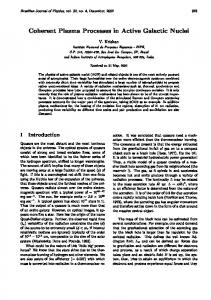
V from [B¨aumer et al., 2003]. The upper panel shows the distribution obtained from the V51 (d,2 He)51 Ti reaction at Elab = 171 MeV, with an energy resolution of 125 keV and θcm ≤ 2o . The lower panel shows the large-scale shell model calculations within the full pf-shell, using the KB3G interaction (see text). The calculated distribution strength is multiplied by an overall quenching factor of (0.74)2 .

the shell gap at the N = 28 magic number, most notably on 56 Ni (≈ 1 MeV excess). Furthermore, it gives a wrong ordering of the single-particle energies in the upper part of the pf-shell, since it pushes the f5/2 orbital above the p-orbitals. In order to extend the shell model calculations above A = 50, a modification of the monopole correction in the KB3 force was introduced (hereafter KB3G interaction) in [Caurier et al., 1999a] and further improved in [Poves et al., 2001]. Calculations within the full pf-shell, using the (SM)2 code together with the KB3G interaction, give an excellent agreement with the few experimentally measured GT distribution strengths and half-lifes for nuclei in the mass range 45 < A < 65 [Caurier et al., 1999a]. As an example, we show in Fig. 3.3 a comparison between the recently 34

measured GT+ distribution strength of 51 V and the one calculated with the (SM)2 code within the full pf-shell [B¨aumer et al., 2003]. The shell model calculations uses the KB3G interaction and were multiplied by an eff /g )2 = (0.74)2 . overall quenching factor (gA A

3.2.2

Shell Model Monte Carlo calculations

The SMMC method is based on a statistical formulation of the nuclear many-body problem. It is described in great detail in [Lang et al., 1993] and [Koonin et al., 1997]. At finite temperatures an observable is calculated as the canonical expectation of an operator Ω at a given nuclear temperature, TN : hΩi =

Tr [Ω U] Tr [U]

(3.10)

where U = exp(−βHN ) is the imaginary-time (β = 1/kB TN ) evolution operator of the many-body nuclear hamiltonian, HN . Tr [U] is the canonical partition function, where the sum is over all many-body states of the Anucleons system. To apply the HS transformation, first we need to realize that the two-body component of the residual interaction can be rewritten as the sum of a one-body component plus a diagonal quadratic form, such that the nuclear hamiltonian reads: HN = H1 + H2 =

X

Eα Λα +

α

1X 0 2 V Λ 2 α α α

(3.11)

where Λα is a one body operator that can be expressed as tensor products of a† and a and Vα0 is the strength of the two-body interaction in the channel α. Since, in general, the different terms of the nuclear hamiltonian do not commute with each other, one divides the imaginary-time β in Nt ”time” 2 slices of length ∆β = β/Nt , such that (∆β) 2 [Λα , Λβ ] ≈ 0 and apply the following gaussian identity to each one of them: e−∆βHN =

Z +∞ Y −∞

α

s

dσα

∆β|Vα0 | − ∆β P |Vα0 |σα2 −∆β P hα α α e 2 e 2π 35

(3.12)

where the hα = (Eα + sα Vα0 σα )Λα

(3.13)

are one-body hamiltonians. The σα are auxiliary fields and sα = ±1 if Vα0 < 0 or sα = ±i if Vα0 > 0. Thus, the global evolution operator is simply written as the product of Nt linearized evolution operators U ≈ U1 × · · · × UNt , in different auxiliary fields. The shell model problem is then transformed from the evaluation of Ns × Ns two-body matrix elements into the evaluation Ns × Ns × Nt one-body matrix integrals. The expectation value of Ω now reads: R

hΩi =

DσWσ Ωσ DσWσ

(3.14)

R

where Wσ = Tr[Uσ ], Ωσ = Tr[Ω Uσ ]/Tr[Uσ ] and Dσ = dσ1 · · · dσNt · · · dσNt Ns2 . The practical way to deal with these large dimensions is to perform the integrations within the Monte Carlo method, using the Metropolis algorithm to generate independent random samples in arbitrary dimensions [Koonin and Meredith, 1998] or [Vetterling et al., 1992]. The Monte Carlo method requires that the weight function Wσ must be real and non-negative. Unfortunately, for most of the realistic interactions and natural decompositions of the nuclear hamiltonian, Vα0 > 0 over some portions of the integration volume and, therefore, Wσ becomes an exponential oscillating function (sα = ±i) in that part of the integration volume. This leads to unacceptable large errors whenever Wσ changes sign. This problem can be circumvented by describing the realistic nuclear hamiltonian by an important class of pairing plus multipole interactions free from the sign problem [Lang et al., 1993]. It has been found that the realistic residual interaction is strongly dominated by a pairing (short-range) and quadrupole (longrange) forces. The pairing plus quadrupole interaction allows for accurate calculations of the many-body problem at finite temperature, including the relevant nuclear properties.

36

Chapter 4

Stellar weak interaction processes Weak interaction processes in the stellar interior are unlike the ones in the laboratory. Stellar weak interaction rates are highly variable due to the large sensitivity to the range of temperatures and densities that occur in stars, while the rates measured in the laboratory are largely determined by fixed atomic parameters [Bahcall, 1964]. In the stellar plasma, atoms are usually fully ionized and electrons form a continuum gas. The degree of degeneracy of the electron gas is strongly dependent on the temperature and density of the matter inside the star. In the final stage evolution of a massive star, electrons are highly degenerate and this has a strong influence on the weak interaction rates. Furthermore, at high temperatures and densities, one can expect that the weak interaction transitions proceed through nuclear states at excitations energies well above the ones involved in laboratory measurements.

4.1

Weak interaction rates in the stellar interior

During the pre-supernova evolution of a massive star, weak interaction processes are dominated by allowed GT transitions. The two main weak 37

interaction processes are the electron capture and the β − -decay: Electron capture: e− +(A, Z) −→ (A, Z −1) + νe

Qec ≈ [M (A, Z) − M (A, Z −1)]c2

β − -decay: (A, Z) −→ (A, Z +1) + e− + ν¯e

Qβ = [M (A, Z) − M (A, Z +1)]c2

where (A, Z) characterizes a nucleus with mass number A and atomic number Z and has a nuclear mass M (A, Z); the Q’s are the reaction Q-values. The relevant transition rates are given by the well known Fermi’s Golden Rule: 2π dλif = |hf |HW |ii|2 dnf (4.1) h ¯ where dnf is the density of final states. The final state neutrino may be considered as a free and massless particle. The number of final neutrino states in a unit volume is then: 1 (4.2) dnν = 2 3 p2ν dpν 2π ¯ h p

where cpν = Eν2 + m2ν c4 ≈ Eν . The final state electron in the β − -decay can not be treated as a free particle, since it is immersed in the Coulomb field of the final nucleus (the same holds for the incoming electron in the capture process). A good approximation may be obtained by starting from the free particle form and folding in a distortion factor F (Z + 1, Ee ) to correct for the Coulomb effects: 1 (4.3) dne = 2 3 F (Z + 1, Ee )p2e dpe 2π ¯ h p

where cpe = Ee2 + m2e c4 . The F (Z, Ee ) is known as the Fermi function; it can be approximated by, ¯ Γ(s + iη) ¯2 ¯ ¯ ¯

F (Z, Ee ) ≈ 2(1 + s)(2pe R/¯ h)2(s−1) eπη ¯ 38

Γ(2s + 1)

p

where s = 1 − (αZ)2 and η = αZEe /(cpe ), α is the fine structure constant and Γ(z) is the Γ-function [Abramowitz and Stegun, 1967]. Neglecting possible corrections due to the presence of bound electrons and ions, the electron gas can be well described by the Fermi-Dirac distribution: fe (Ee ) =

1 1 + exp(Ee − µe )/kB T

(4.4)

In our calculations the electron chemical potential was derived from the matter density and temperature by inverting the relation: ρYe =

1 2 π NA ¯h3

Z ∞ 0

[fe (Ee ) − fp (Ee )]p2e dpe

(4.5)

where NA is the Avogadro’s number and fp (Ee ) is the Fermi-Dirac distribution for positrons. This distribution is defined with µ+ e = −µe , where + µe stands for the positron chemical potential. The total rate between an initial (parent) nuclear state and a final (daughter) nuclear state is then obtained by integrating eq. (4.1) over the electron energy, folded with the Fermi-Dirac distribution and summing the two electron spin orientations. Using the definitions (2.8), the weak interaction rates then read: λif =

ln 2 Bif Φif K

(4.6)

where K = 2π 3 (ln 2)¯ h7 /(m5e c4 G2F cos2 θc ) ≈ 6146 s sets the scale of the weak interaction rates and Φif is the phase-space integral. For electron capture, it reads: Φec if

1 = (me c2 )5

Z ∞ E0

if Ee2 (Qec+EX +Ee )2 G(Z, Ee )fe (Ee )dEe

(4.7)

if if with Eνif = Qec + EX + Ee , where EX = Ei − Ef is the energy difference between the excitation energies of the parent and daughter states and E0 ≥ 0 is the threshold energy for electron capture. It can be E0 = 0 if if if ) otherwise. We also define: ≥ 0 or E0 = −(Qec + EX Qec + EX

G(Z, Ee ) =

cpe F (Z, Ee ) Ee

(4.8) 39

For supernova conditions, electrons are relativistic, such that G(Z, Ee ) ≈ F (Z, Ee ). For β − -decay, the phase-space integral reads: − Φβif =

1 (me c2 )5

Z ∞

if Ee2 (Qβ +EX −Ee )2 G(Z+1, Ee )[1−fe (Ee )]dEe (4.9)

me c2

if with Eνif = Qβ + EX − Ee . The corresponding phase-space integrals for positron capture and β + -decay are straightforward [Fuller et al., 1980]. In these expressions we neglect any Pauli blocking resulting from the degeneracy of the final state neutrinos. This only happens at later stages of core collapse, when densities are a few 1011 gcm−3 and neutrino trapping sets in. It can be accounted for by including a neutrino blocking distribution, [1 − fν (Eν )], in the integrand of the phase-space integrals. The phase-space integrals comprise the extreme sensitivity of the weak interaction rates to variations of temperature and density. To facilitate extrapolations it is usual to express them in terms of so-called f t-values, which are defined by:

λif = ln 2

Φif (f t)if

or

(f t)if =

K Bif

(4.10)

The reduced transition strength Bif is in principle given by the sum of 2 B (GT ). However, the Fermi and GT contributions, Bif = Bif (F ) + gA if nuclei relevant in the supernova evolution have N ≥ Z and, hence, Fermi transitions for electron captures (as well as for β + -decay) are not allowed, since the isospin difference between the daughter and parent states is always ∆I ≥ 1 in this case. Fermi transitions for β − -decays (as well as for positron captures) are allowed, but not necessarily possible due to energy reasons.

4.1.1

Nuclear excitation in the supernova environment

At finite temperature, one can expect the thermal population of many nuclear excited states in the parent nucleus. The total weak interaction transition rate is then given by the thermal average of all transition rates from states in the parent nucleus to states in the daughter nucleus: λ=

X Wi if

W

λif

with

Wi = (2Ji + 1) exp(−Ei /kB T ) 40

(4.11)

P

and W = i Wi is the nuclear partition function. At low temperature and density regimes, a reliable description of the stellar weak interaction rates can be obtained by considering explicitly just the low-lying states, but, with increasing temperature and density, states at higher excitation energies become important. A state-by-state evaluation of all transition rates, connecting excited states in parent nucleus with states in the daughter nucleus, is not feasible with the present computer capabilities. GT transitions from excited states in the parent nucleus to the low-lying states in the daughter nucleus are important for stellar weak interaction rates and particularly for β − -decay, as it was pointed out in [Aufderheide et al., 1994a]. These transitions are known as back-resonances and their importance arises from the large matrix elements and increased phase-space associated with them. They can be easily obtained from the low-lying states in the daughter nucleus using detailed balance. For example, in Fig. 4.1, the β − -decay (electron capture) back-resonances can be obtained by inverting the GT+ (GT− ) matrix elements that connect the low-lying states in the daughter nucleus with the resonances at high excitation energies in the parent nucleus. The importance of the backresonances was first recognized by Fuller, Fowler and Newman (hereafter FFN) in their pioneering and systematic study of stellar weak interaction rates [Fuller et al., 1980, Fuller et al., 1982a, Fuller et al., 1982b]. In their work they estimate the weak interaction rates for nuclei with 21 ≤ A ≤ 60 for pre-supernova and early-stage core collapse conditions. The GT collective modes were estimated by a parametrization based on the IPM. The rates were then completed with the inclusion of Fermi transitions when applicable and experimental data for the low-lying GT states, whenever available. An empirical value of ln(f t) = 5 was assigned to these states, whenever these data were experimentally unknown. By the time the FFN rates were calculated the quenching of the GT strength had not been established. Later, in [Fuller et al., 1985], the authors pointed out this effect and gave a way to effectively incorporate the quenching into the rates.

41

4.1.2

Large-scale shell model calculations of stellar weak interaction rates

Recently, new calculations of the weak interaction rates (hereafter LMP) were performed based on the (SM)2 code antoine for more than 100 nuclei in the 45 ≤ A ≤ 65 mass region [Langanke and Mart´ınez-Pinedo, 2001]. These calculations were done within the full pf-shell with a truncation level at which the GT strength distributions were virtually converged, using the monopole-modified KB3G interaction [Caurier et al., 1999a]. To account for the quenching of the GT strength, an effective axial coupling constant eff = 0.74 × g was used. The GT strength distributions built on the lowgA A lying states in the parent nucleus were calculated explicitly with the (SM)2 code and the mid back-resonances contributions were included through the detailed balance method. This procedure does not exhaust, however, the total GT strength built on an excited state in the parent nucleus, since there are back-resonances transitions to low-lying states in the daughter nucleus that are not included in the shell model calculations. To correct for these missing transitions, the LMP calculations employed the so-called Brink hypothesis. The Brink hypothesis states that the GT strength distribution on the daughter nucleus of an excited state (with an excitation energy Ei ) in fi the parent, S i (EX ), is the same as for the ground-state, but shifted by the fi fi excitation of the parent nucleus: S i (EX ) = S 0 (EX + Ei ) = S 0 (Ef ). The Brink hypothesis has been proven valid for the bulk of the GT distributions, but it can fail for specific transitions at low excitation energies. However, at finite temperatures, many states will contribute in a way that variations in the low-lying transitions tend to average out and the Brink hypothesis becomes a valid assumption [Fuller et al., 1982a]. The LMP electron capture rates are, in general, smaller than the FFN rates. This trend results from the quenching of the GT strength and a systematic displacement of the centroid of the GT distribution. It was found that the GT distributions are centered at higher excitation energies for odd-A and odd-odd nuclei than assumed by FFN, while, they are centered at lower excitations energies for even-even nuclei. Two other important reasons that account for differences between the two sets of compi42

Ex (MeV)

Ex (MeV)

15 10 GTGR Ba c

10

kre

so

na

nc es

GT− 5

GTGR

s

IAS

GT+

F 0

Ba

ck

res

on

an

ce

5

0

Q ec

(A,Z)

β−decay

(A,Z−1)

Figure 4.1: Schematic representation of the electron capture process on a nucleus (A, Z) and β − -decay of a nucleus (A, Z − 1). In the supernova environment, the electron capture process is dominated by the excitation of the GT+ strength in the daughter nucleus (A, Z − 1), whereas, the β − -decay is dominated by of the GT− strength and the Fermi strength (concentrated in the IAS) in the daughter nucleus (A, Z). The dashed lines represent the back-resonances that account for transitions from excited states in the parent nuclei to the low-lying states in the daughter nuclei (see text).

43

lations are the fragmentation of the GT distribution obtained in the shell model calculations and that was not considered in the FFN parametrization and improvements on the knowledge of Q-values for some specific nuclei [Langanke and Mart´ınez-Pinedo, 2000]. The captures to the bulk of the GT+ strength in odd-A and odd-odd nuclei are energetically less favored in the LMP calculations than in the parametrization by FFN. The rates for electron captures on even-even nuclei were found to be about the same as in the FFN calculations, as the empirical low-lying strength used in the later compensates the decrease in energy of the GT+ centroid obtained by LMP. These displacements have also important consequences for the β − -decay rates. The excitation of the back-resonances in even-even and odd-A nuclei (the daughters of electron captures on odd-odd nuclei) becomes less likely – but still important – for the pre-supernova conditions, whereas, for odd-odd nuclei (the daughters of electron captures on even-even nuclei), the LMP calculations show that the back-resonances reside at lower excitation energies than previously parameterized [Langanke, 1999]. The consequences of the new rates (including electron captures, β − decays, positron captures and β + -decays) in the pre-supernova evolution of massive stars were studied in [Heger et al., 2001]. These studies show that β − -decays can compete with electron captures on nuclei. This has two main reasons: (i) the general decrease of the electron capture rates found in the LMP calculations and (ii) the increase of the β − -decay rates, due to the thermal excitation of the back-resonances and the evolution of the nuclear matter towards neutron-rich nuclei that favors the β − -decay processes relative to the electron captures, as Qβ decreases and |Qec | increases. The new models show important changes in relevant physical properties (the lepton fraction, the central entropy and the size of the iron core) of the star at the onset of core collapse relative to previous ones (for example, [Woosley and Weaver, 1995]). The competition between electron captures and β − -decays is, however, mostly sensitive to the degeneracy of the electron gas and ultimately β − -decays become completely Pauli blocked with increasing temperature and density, as the star enters the core collapse phase. 44

4.2

Neutrino spectra from electron captures (1)

In chapter 1, we mentioned how electron captures on iron group nuclei produces large amounts of neutrinos. Subsequent neutrino interactions play a fundamental role during the core collapse phase. Therefore, supernova simulations require a detailed bookkeeping of neutrino spectra from electron captures. Core collapse simulations have been performed using stellar weak interaction rates based on a simple parametrization of the GT strength first introduced in [Bethe et al., 1979] and later used in [Bruenn, 1985]. This parametrization assumes an IPM that only considers GT transitions between the 1f7/2 and 1f5/2 orbits and that the GTGR in the daughter nucleus is at an excitation energy of 3 MeV for any nucleus. In Bruenn’s work, the corresponding neutrino spectra were derived assuming that: (i) the electron capture on the parent nucleus ground-state leads to a single state in the daughter nucleus at an energy Ef and, (ii) if the capture is on an excited state in the parent at an excitation energy, Ei , then the final state in the daughter is at an energy Ef + Ei (this is just a restatement of the Brink hypothesis). The resulting neutrino spectrum is:

n(Eν ) = Eν2 (Eν − q)2

N 1 + exp(Eν − q − µe )/kB T

(4.12)

if . The parametrizawhere N is the normalization constant and q = Qec +EX tion by Bruenn is q = Qec − 3 MeV.

A more reliable treatment of the nuclear structure is now possible on the basis of large-scale shell model calculations. In the next subsection, we will present the neutrino spectra from stellar electron captures derived from the LMP calculations of the GT distributions for iron group nuclei, including the back-resonances contribution. We will also provide a way to easily implement them in core collapse codes. 45

4.2.1

Results and discussion

The normalized shell model neutrino spectra were calculated dividing the partial rate per energy interval by the total rate: n(Eν ) =

λec (Eν ) λec

with

λec =

Z ∞ 0

λec (Eν )dEν

(4.13)

where λec (Eν ) is given by the sum of all i → j transitions between parent and daughter states leading to the same final neutrino energy Eν . The spectra for the A = 56 isobars are shown in Fig. 4.2, for typical conditions during silicon burning of a 15M¯ star (T = 4 × 109 K, ρ = 3×108 gcm−3 and Ye = 0.45). For these conditions we obtain µe = 2.5 MeV. With the exception of 56 Co, all other isotopes have similar spectra, peaked around Eν ≈ 1 − 2 MeV with a width about 1.4 − 1.8 MeV. For nuclei with negative Q-values, like 56 V (Qec = −7.6 MeV), 56 Cr (Qec ≈ −9.6 MeV), 56 Mn (Q 56 Fe (Q ec ≈ −2.2 MeV) and ec ≈ −4.2 MeV), electron captures require the high-energy electrons from the tail of the Fermi-Dirac distribution, fe (Ee ). Obviously, appreciable rates are obtained from electrons with lower energy and, hence, for small neutrino energies. For 56 Ni, the Q-value is positive (Qec ≈ 1.6 MeV) and, consequently, capture is possible for all electron energies, however, the GT+ is found to be well concentrated at low excitation energies (Ef ≈ 3.4 MeV) in the daughter nucleus, 56 Co, resulting in a narrow spectrum. The 56 Co spectrum is quite different, showing a double-bump. To investigate the origin of this structure, we calculated the partial contributions for the total spectrum. These are shown in Fig. 4.3. The spectra from captures on the ground-state (Ji = 4) and 1st excited state (Ji = 3) have the normal single-peaked structure. The 1+ excited state at Ei = 1.7 MeV excitation energy produces a neutrino spectrum with a peak around Eν ≈ 8 MeV. This state has a strong GT+ matrix element to the ground-state of 56 Fe that, combined with the positive Q-value (Qec ≈ 4.1 MeV), generates neutrinos with rather large energies. Although the excitation energy in the parent increases the effective Q-value (Qec + Ei ≈ 5.8 MeV), the contribution of the GT strength to the rate is reduced by the Boltzmann weight in eq. (6.8). 46

0.8 56

V

56

Cr

56

Mn

Fe

56

Co

56

Ni

0.6

n (MeV-1)

0.4 0.2 0 56

0.6 0.4 0.2 0

0

2

4

6

8

10

0

2

4

6

8

10

0

2

4

6

8

10

12

Eν (MeV)

Figure 4.2: Normalized neutrino spectra from stellar electron captures on selected A = 56 isobars. The spectra have been calculated for typical conditions during the silicon shell burning in a 15M¯ star [Heger et al., 2001]. The stellar parameters are T = 4 × 109 K, ρ = 3 × 108 gcm−3 and Ye = 0.45 (µe = 2.5 MeV).

Further important contributions arises from the back-resonances that connect the excited states in 56 Co, around Ei ≈ 2 − 4 MeV, with the low-lying states in the daughter nucleus, 56 Fe. Despite the Boltzmann suppression, the combined large matrix elements together with the gain in phase-space produces the second peak in the neutrino spectrum. Electron captures on the odd-odd nuclei 56 Mn and 56 V do not produce the double-bump due to their negative Q-values that favors the emission of low-energy neutrinos. For the silicon burning conditions taken above, the electron chemical potential is yet not large enough to allow significant captures from the low-lying states in 56 Co to the bulk of the GT+ , which reside at Ef ≈ 7−9 MeV in 56 Fe. This increases the relative weight of the back-resonances for these stellar conditions. With the subsequent stellar evolution, the 47

0.4

ground state first exc. state 1+ exc. state backresonances total

n (MeV-1)

0.3

0.2

0.1

0 0

1

2

3

4

5

6

7

8

9

10

Eν (MeV)

Figure 4.3: Partial contributions of individual states to the neutrino spectrum from stellar electron capture on 56 Co (Qec ≈ 4.1 MeV). The calculation were performed for the same conditions as in Fig. 4.2. The spectra are multiplied by their relative weight to the total capture rate.

electron chemical potential increases substantially and the capture from the low-lying states to the bulk of the GT+ strength becomes possible, producing neutrinos with larger energies. The relative importance of the back-resonances decreases despite a gain in the Boltzmann factor with the increasing temperature. This behavior is shown in Fig. 4.4 for a late-stage stellar trajectory of a 15M¯ star, obtained from [Heger et al., 2001]. The last two panels show the transition to the regime where the capture to the bulk of the GT+ distribution dominates the rate completely and, hence, the spectra become single-peaked. The first panel represents the regime of low temperatures and low chemical potentials. Here, the spectrum is also single-peaked, as the rate is dominated by the capture on a single state – the ground-state of 56 Co. The spectrum also shows “discontinuities” that reflect the sensitivity of the spectrum to transitions to individual states in the daughter nucleus. For larger µe , these discontinuities are smeared out 48

0.5 µe=0.9

0.4

T9=2.25

µe=1.3 T9=3.39

µe=1.5 T9=3.82

µe=2.5 T9=4.13

µe=4.2 T9=4.41

µe=8.1 T9=7.25

0.3

n (MeV-1)

0.2 0.1 0.0 0.4 0.3 0.2 0.1 0

0

2

4

6

8

10

0

2

4

6

8

10

0

2

4

6

8

10

12

Eν (MeV)

Figure 4.4: Normalized neutrino spectra for stellar electron capture on

56

Co for different conditions in the late-stage stellar evolution of a 15M¯ star. The stellar parameters were taken from [Heger et al., 2001]. The chemical potentials are given in MeV and T9 defines the temperature in 109 K.

as the spectra from transitions to individual states overlap. In Fig. 4.5, the spectra from electron captures in 56 Fe do not show the double-bump structure for any stellar condition. This behavior is the result of the displacement of the centroids of the GT distribution mentioned before. The back-resonances, for electron captures on an even-even nucleus like 56 Fe, are at higher excitation energies (≈ 3 MeV) than on an odd-odd nucleus like 56 Co. Transitions from low-lying states to the bulk of GT+ dominate the rates at the energies required to capture from the backresonances in a even-even nucleus and, therefore, the spectra are singlepeaked. The capture at low chemical potentials proceeds from low-lying states in 56 Fe to low-lying states in the daughter nucleus, 56 Mn, resulting in a neutrino spectrum with a narrow peak at low energies. With increas49

0.8 0.6

µe=1.3 T9=3.39

µe=1.5 T9=3.82

µe=2.5 T9=4.13

µe=4.2 T9=4.41

µe=8.1 T9=7.25

µe=11.6 T9=10.0

n (MeV-1)

0.4 0.2 0.0 0.6 0.4 0.2 0

0

2

4

6

8

10

0

2

4

6

8

10

0

2

4

6

8

10

12

Eν (MeV)

Figure 4.5: Normalized neutrino spectra for stellar electron capture on

56

Fe for different conditions in the late-stage stellar evolution of a 15M¯ star. The stellar parameters were taken from [Heger et al., 2001]. The last panel corresponds to typical conditions during the collapse phase (T = 7.2 × 109 K, ρ = 9.1 × 109 gcm−3 and Ye = 0.43). The chemical potentials are given in MeV and T9 defines the temperature in 109 K.

ing electron chemical potential, the spectra move towards higher neutrino energies and gets wider, as the result from the capture to the bulk of the GT+ distribution. For the collapse conditions as shown in the last panel of Fig. 4.5, electron captures on the relevant nuclei produce the simple single-bump structure. Fig. 4.6 shows the neutrino spectra for six nuclei that dominate electron captures in the pre-supernova model of 15M¯ star [Heger et al., 2001]. The temperature and density are T = 7.2 × 109 K and ρ = 9.1 × 109 gcm−3 , while, Ye = 0.43. The electron chemical potential is then µe = 8.1 MeV. The average neutrino energy released by the nuclei is about 3 MeV, while 50

0.4 1

H

52

V

62

Co

59

Fe

65

Ni

0.3

n (MeV-1)

0.2 0.1 0 63

Ni

0.3 0.2 0.1 0

0

2

4

6

8

10

0

4

2

6

8

10

0

2

4

6

8

10

12

Eν (MeV)

Figure 4.6: Normalized neutrino spectra from stellar electron capture on the six most important “electron-capturing” nuclei in the pre-supernova model of a 15M¯ star. The stellar parameters are T = 7.2 × 109 K, ρ = 9.1 × 109 gcm−3 , Ye = 0.43, (µe = 8.1 MeV). The solid lines represent the spectra derived from the large-scale shell model calculations. The dashed lines shows the fit to the spectra, using the parametrization of eq. (4.12) and adjusting q to the average neutrino energy of the spectra from the large-scale shell model spectra. The dashed-dot spectra corresponds to the parametrization of Bruenn q = Qec − 3 MeV [Bruenn, 1985].

it is about 6 MeV for capture on free protons. The spectra can be well approximated by eq. (4.12). For electron captures on free protons, the parameter q is the reaction Q-value, q = −1.29 MeV. For finite nuclei, we considered q as a fit parameter adjusted to the average neutrino energy. A code has been implemented to give the q-parameter for a given nucleus and temperature-density (ρYe ) points. This proposal reproduces, in general, the large-scale shell model calculations of the spectra rather well, as it can be seen by the dashed curves in Fig. 4.6. We note, however, that for 52 V, the shell model spectrum is wider than the 51

parametrization. This is due to the fact that some specific states in this nucleus do not follow the Brink hypothesis as assumed in deriving eq. (4.12). For example, the excited state of 52 V (Qec = −2.5 MeV) at Ei ≈ 22 keV has Ji = 5 and can only connect with states with Jf = 4, 5 and 6 in the daughter nucleus, 52 Ti. The state with Jf = 4 corresponds to the one at lowest excitation energies, but still the large GT+ resonances built on this if state are at EX ≈ 6 − 8 MeV. Thus, even for collapse conditions, these resonances can not be reached. On the other hand, the excited state Ji = 1 at 141 keV connects with a large matrix element to the ground-state of 52 Ti. We also note that Bruenn’s parametrization (q = Qec − 3 MeV), although simple, gives an acceptable agreement with some nuclei.

52

Chapter 5

Neutrino-induced reactions on nuclei Neutrino-induced

reactions play a fundamental role in the late-stage core-collapse phase and post-bounce evolution of the shock-wave in a supernova. Supernova simulations have incorporated a number of neutrinoinduced reactions on electrons, free nucleons and nuclei. Neutrino absorption reactions on nuclei have been derived by detailed balance from electron capture reactions within the parametrization used in [Bruenn, 1985]. So far, inelastic neutrino-nucleus reactions have been ignored in the simulations. In 1988, Haxton argued that the excitation of the nuclear giant resonances in the supernova environment can lead to significant cross sections of inelastic neutrino-induced reactions on nuclei and this effect should, therefore, be added in supernova simulations [Haxton, 1988].

5.1

Introduction

The effects of neutrino charged- and (inelastic) neutral-currents reactions on nuclei were studied in [Bruenn and Haxton, 1991] for the collapse phase, prompt shock propagation phase and delayed shock phase. In their studies, 56 Fe was taken as the solely representative nucleus during the three phases. 53

The cross sections were evaluated for the ground-state of 56 Fe, including allowed and 1st forbidden transitions. The ground-state nuclear response was determined by diagonalising the KB interaction G-matrix, including all 2p–2h excitations of a closed 56 Ni core. The model-space was then expanded to include all 3p-3h excitations and fully diagonalized to generate the spectra of excited states for 56 Fe, 56 Mn and 56 Co. The GDR resonance in 56 Fe which dominates the 1st forbidden transitions was described by the Goldhaber-Teller model. It was found that neutrino-nucleus inelastic scattering rates are not negligible during the collapse. The neutrino-nucleus absorption rates were found to be too small to have an appreciable effect. The neutrino absorption reaction has to overcome the Q-value (Qβ ≈ −4.6 MeV) that strongly hinders this process at low energies. For neutrino inelastic scattering there is not a Q-value, but there is an energy gap between the ground-state (Ji = 0) of 56 Fe and the first allowed final state (Jf = 1) that similarly reduces the low-energy cross sections for this process. In the supernova environment, one must note that cross sections of neutrino reactions on the ground-sate of 56 Fe are not representative of all relevant neutrino-nucleus reactions. This has two reasons: (i) Most of the nuclei present in the composition during the collapse do not exhibit a finite energy threshold. These are neutron-rich nuclei and in general the (νe , e− ) processes have positive Q-values. Many of these are odd-odd and odd-A nuclei for which sizable GT transitions are possible at smaller excitation energies than for even-even nuclei. (ii) During the collapse, neutrino reactions occur at finite temperature for which the thermal population of nuclear excited states is expected to be important. Transitions from these states to low-lying final states (back-resonances) can remove effectively the ground-state threshold in both charged- and neutral-current reactions and contribute to the enhancement of neutrino-nucleus cross sections at low energies. The importance of the thermal nuclear excitation was already noticed in [Fuller and Meyer, 1991]. This work assumes that the nuclear response at a given temperature can be represented by a single excited nuclear configuration with an average energy given by the Fermi gas model. This energy was then used to compute the total strength of the neutrino-nucleus inter54

action – where the nucleus was represented by 56 Fe – within the framework of the IPM, including allowed and forbidden single-particle transitions. Below kB T ≈ 5 MeV, the rates were found to be dominated by the 1f5/2 -1f7/2 transitions, where an energy splitting of 6.5 MeV was taken between these two orbits. Consequently, for the temperatures relevant during core collapse (kB T ≈ 1 MeV), the effects were found to be negligible and only became significant at kB T ≥ 5 MeV, when GT transitions can overcome this energy threshold and also forbidden transitions start to contribute. The role of finite temperature in low-energy (Eν < 15 MeV) neutrino reactions on nuclei can be studied more accurately on the basis of the shell model calculations calculations of the GT transitions, which dominate the nuclear response at these energies. In this chapter, we will present the neutrino absorption (charged-current) reactions and inelastic scattering (neutral-current) reactions, Charged-current: νe +(A, Z) −→ (A, Z +1) + e− ν¯e +(A, Z) −→ (A, Z −1) + e

+

Q− = Qβ Q+ ≈ Qec

Neutral-current: ν +(A, Z) −→ (A, Z)? + ν 0 on representative neutron-rich nuclei (A ≈ 60) around kB T ≈ 1 MeV, derived from the LMP calculations of the GT strength distributions. Finite momentum transfer dependence of the transition matrix elements was neglected in our calculations. Reactions on even-even, odd-odd and odd-A nuclei were considered in the study.

5.2

Neutrino reaction cross sections in the supernova environment

The cross sections for these processes follow directly from the formalism shown in the last chapter. They read: 55

Charged-current: σ± (Eν ) =

G2F cos2 θc eff 2 X if 2 Wi (gA ) (Ee ) G(Z ± 1, Eeif )Bif (GT± ) π W if (5.1)

Neutral-current: σ0 (Eν ) =

Wi G2F eff 2 X if 2 (g ) (Eν 0 ) Bif (GT0 ) π A W if (5.2)

where W is the nuclear partition function defined in the last chapter. The energy of the outcoming electron in charged-current reaction is Eeif = Eν + if Q∓ + EX and the energy of the outcoming neutrino in the neutral-current if reaction is Eνif0 = Eν + EX . These cross sections were evaluated assuming the Brink hypothesis. Under this assumption, the nuclear transitions are independent of the initial state and consequently the cross sections become independent of the temperature, as one can see in the following: X

fi ) Bif (EX

if

X Wi X Wi X = B0f (Ef ) = B0f (Ef ) W W i f f

In our model, we include, however, the thermal excitation of the backresonances. Thus, eqs. (5.1) and (5.2) can be split into two terms: Charged-current: 

G2 cos2 θc eff 2 X 0f 2 σ± (Eν ) = F (gA ) (Ee ) G(Z ± 1, Eeif )B0f (GT± ) π f 

+

X if

Wi back (Eeif )2 G(Z ± 1, Eeif )Bif (GT± )  W 56

(5.3)

Neutral-current: σ0 (Eν ) =

+

X if

G2F π

 X (g eff )2  (E 0f0 )2 B0f (GT0 ) A

ν

f



Wi back (Eνif0 )2 Bif (GT0 )  W

(5.4)

The temperature dependence of these cross sections is comprised solely in the back-resonances terms. In our calculations, the back-resonances were obtained from the lowest daughter (final) states through the detailed balance method using the proper geometrical factor: back Bif (GT0,± ) =

2Jf + 1 Bf i (GT0,± ) 2Ji + 1

(5.5)

back ) transitions that connect these daughter states with the parent The (B0f ground-state have been eliminated in the back-resonances contribution to avoid double counting. Neutrino absorption cross sections at finite temperatures and high densities can be strongly reduced by the phase-space Pauli blocking of the final state electrons. To account for this effect, we multiplied the charged-current cross sections by an electron blocking distribution, given by 1 − fe (Ee ), where f (Ee ) is the Fermi-Dirac distribution defined in eq. (4.4). For final state positrons, the blocking distribution is defined in the same way with µe+ = −µe .

5.2.1

Charged-current neutrino absorption reactions: results and discussion (2)

For the discussion we now consider neutrino absorption reactions on a few selected nuclei. The neutrino-nucleus cross sections on these nuclei were evaluated for three stellar temperatures, kB T = 0.86, 1.29 and 1.72 MeV. These correspond, roughly, to three stages in the evolution of the collapse. The first is the pre-supernova condition of a 15M¯ star and the 57

other two are, respectively, the neutrino trapping and neutrino thermalization conditions. For comparison, we also evaluated the ground-state cross sections to simulate the T = 0 condition. To understand the role of the two terms in eq. (5.3), we studied the 56 Fe(ν , e− ) reaction in several steps. In Fig. 5.1(a), we compare the grounde state cross section with the one obtained including explicitly the four lowest states in 56 Fe (no Brink hypothesis assumed), but not including the back-resonances contribution. We find almost the same results in both approaches, indicating that the Brink hypothesis is a good approximation for these low-lying states. Fig. 5.1(b) shows the charged-current cross sections in 56 Fe obtained from eq. (5.3). The bulk of the GT+ back-resonances strength in 56 Fe is located at an excitation energy of Ei ≈ 9 − 11 MeV. Therefore, the cross section starts to be sensitive to the back-resonances below Eν = Q− + Ei ≈ 5 − 7 MeV. For neutrino energies above this value, the ground-state (Brink) transitions in our model dominate and the cross section becomes temperature-independent. Despite the negative Q-value (Q− ≈ −4.6 MeV), the cross section does not vanish at Eν = 0, since it is possible to capture from the back-resonances. Finally, we evaluated the same cross sections, but now including the blocking of the final state electron as described above. The chemical potentials were computed using eq. (4.5) for the stellar conditions summarize in Tab. 5.1 [Bruenn and Haxton, 1991]. Fig. 5.1(c) shows that neutrino absorption cross sections are strongly suppressed due to the Pauli blocking of the final state electron. Scattering through the back-resonances gives an additional energy to the outcoming electron. Consequently, it is less affected by the blocking, however, as the chemical potential grows much faster than the temperature, the thermal population of the back-resonances can not compete with blocking. At Eν = 0, cross sections are strongly enhanced relative to the ground-state result, but they are significantly smaller than the competing processes of inelastic scattering on electrons and nuclei. Now we turn our discussion to more neutron-rich nuclei. We have chosen 59,61 Fe as representatives of odd-A nuclei and 60,62 Co as representatives of odd-odd nuclei. In Fig. 5.2, we show the temperature dependence of the electron neutrino absorption cross sections for these nuclei. In all cases, we 58

3 (a) 0 -3 -6

2

3

-42

cm )]

-9

0 -3

e

Log10[σν (10

(b)

ground-state kBT=0.86 kBT=1.29 kBT=1.72

-6 -9 3 (c) 0 -3

ground-state kBT=0.86, µe=8.3

-6

kBT=1.29, µe=18.1

-9 -12

kBT=1.72, µe=36.2 0

5

10

15

20

Eν (MeV) e

Figure 5.1: Absorption cross section of electron neutrinos in 56 Fe. Temperatures, kB T , and chemical potentials, µe , are in MeV. (a) Comparison of the ground-state cross section with the one obtained at kB T = 0.86 MeV. The calculations have been performed with the 4 lowest states in 56 Fe included explicitly in the thermal ensemble. (b) Comparison of the cross section at three finite temperatures (see text) with the ground-state cross section. The finite-temperature calculations were performed using eq. (5.3) without final state electron blocking. (c) The same as in (b), but now considering the final state electron blocking. The electron chemical potentials are defined in Tab. 5.1.

59

T (1010 K) 1.0 1.5 2.0

kB T (MeV) 0.86 1.29 1.72

ρ (1010 gcm−3 ) 1 10 100

Ye 0.45 0.45 0.35

µe (MeV) 8.3 18.1 36.2

Table 5.1: Stellar parameters for a 15M¯ star [Bruenn and Haxton, 1991]. The electron chemical potentials were derived from eq. (4.5).

obtain an enhancement at low neutrino energies, however, the cross sections are much less temperature-dependent than for even-even nuclei. This has three reasons: (i) These nuclei have small or positive Q-values and, hence, ground-state transitions are possible with any incoming neutrino energy. Only at rather low energies, the thermal population of the back-resonances becomes competitive with these transitions. (ii) As described in the last chapter, the GT+ strength in even-even nuclei is systematically displaced at lower energies compared to odd-A and odd-odd nuclei. This implies that the back-resonances in odd-A and odd-odd nuclei (built from the GT+ in even-even nuclei) lies at significantly lower excitation energies (Ei ≈ 1 − 3 MeV for the odd-odd and Ei ≈ 1 − 5 MeV for the odd-A nuclei) than for even-even nuclei. For example, we can estimate the energy for which the back-resonances start to dominate over the ground-state transitions in 60 Co (Q− ≈ 2.8 MeV). Roughly this energy is then Q− + Ei ≈ 4 − 6 MeV, which is lower than the 5 − 7 MeV for 56 Fe. (iii) From Fig. 5.2, it is also clear that the cross sections become more temperature-independent with increasing (N − Z). This a consequence of the Ikeda sum rule stated in eq. (2.10). The GT− strength for the (νe , e− ) direction increases relative to the GT+ strength for the inverse direction with (N − Z). That is, the ground-state contribution also increases relative to the back-resonances with increasing neutron excess. For the collapse conditions, the electron neutrino cross sections are dom60

2

59

61

Fe

Fe

2

cm )]

0

2 60

e

Log10[σν (10

-42

-2

62

Co

Co

0 ground-state kBT=0.86 kBT=1.29 kBT=1.72

-2

-4

0

5

10

15

0

Eν (MeV)

5

10

15

20

e

Figure 5.2: Absorption cross sections of electron neutrinos on selected neutronrich nuclei. Temperatures, kB T , are in MeV. The calculations have been performed on basis of eq. (5.3) and for the stellar conditions shown in Tab. 5.1.

inated by the final state electron Pauli blocking. This is shown in Fig. 5.3. Despite the fact that cross sections are enhanced by ≈ 2 orders of magnitude relative to the ground-state, they can not compete with inelastic neutrino scattering on electrons and nuclei. Neutrino absorption at higher energies become important with increasing densities during the collapse phase, but our calculations show that temperature effects are negligible. Antineutrino absorption reactions Antineutrinos are not expected to be present during the collapse phase. Nevertheless, we calculated the electron antineutrino absorption cross sections for the same set of nuclei. The results are shown in Fig. 5.4. To understand them, we can use the same arguments listed before, but re61

4

59

61

Fe

Fe

2

cm )]

0

e

Log10[σν (10

-42

-4

-8 4

60

62

Co

Co

0 ground-state kBT=0.86, µe=8.3

-4

kBT=1.29, µe=18.1 kBT=1.72, µe=36.2

-8 0

10

20

30

40

0

10

Eν (MeV)

20

30

40

50

e

Figure 5.3: The same as in Fig. 5.2, but now including the final electron Pauli blocking distribution. Temperatures, kB T , and chemical potentials, µe , are in MeV.

versely. (i) The Q-values are negative and, therefore, the reactions have to overcome sizable thresholds. This effect increases with neutron excess, as the final positron phase-space decreases. (ii) The GT− strengths of the back-resonances lies at lower excitation energies for odd-A and odd-odd nuclei than for even-even nuclei. (iii) The Ikeda sum rule asserts that the GT+ strength for the (¯ νe , e+ ) decreases relative to the GT− for the backresonances with (N −Z). The sum of these effects leads to a very noticeable enhancement of the cross sections relative to ground-state calculations below 10 MeV. Furthermore, the final positron blocking is absent, for these stellar conditions, due to the negative chemical potential. This is a hint for the neutral-current reactions, where the population of the back-resonances is expected to be important at finite temperatures and the neutrino chemical potential negligible for the same conditions. 62

2

59

61

Fe

Fe

-2 -4

Log10[σν_ (10

-42

2

cm )]

0

2

e

60

62

Co

Co

0 ground-state

-2

+

kBT=0.86, µe =-8.3 +

kBT=1.29, µe =-18.1

-4

+

kBT=1.72, µe =-36.2 -6

0

5

10

15

0

Eν_ (MeV)

5

10

15

20

e

Figure 5.4: Absorption cross sections of electron antineutrinos, including the final state positron blocking. Temperatures, kB T , and chemical potentials, µ+ e , are in MeV. The chemical potentials were derived from eq. (4.5). The final positron blocking is negligible for these stellar conditions.

5.2.2

Neutral-current neutrino scattering cross sections: results and discussion (3)

The first and second terms in eq. (5.4) correspond, respectively, to neutrino down-scattering (Eν 0 < Eν ) and neutrino up-scattering (Eν 0 > Eν ). Neutrino down-scattering is described by the ground-state contribution of the cross section, assuming the Brink hypothesis. It is, therefore, independent of temperature, whereas, neutrino up-scattering is described by the back-resonances term and, therefore, dependent on temperature. For neutral-current reactions it is meaningless to talk about Q-values and Ikeda sum-rule. The understanding of the role of finite-temperature effects is based on the influence of the nuclear pairing structure on the cross sections. We, therefore, start by discussing aspects of the GT0 distributions 63

built on the ground-state of the same set of four nuclei, 59,61 Fe and 60,62 Co. These are shown in Fig. 5.5. The ∆I = 1 component has a much lower total strength than the ∆I = 0 component. This is due to the geometrical factor (Clebsch-Gordan coefficient) that relates the GT0 matrix element to its reduced matrix element, ¯ ¯ · ¸2 ¯ hII − 1|GT0 |IIi ¯2 ¯ ¯ = (II1 − 1|II − 1) = 1 ¯ hII|GT |IIi ¯ (II10|II) I 0

Accordingly, the reduction is larger for nuclei with larger excess (N − Z) = 2I. Moreover, the resonances of the ∆I = 1 component reside at such high excitation energies that they can not be reached by low-energy downscattering neutrinos and they are thermally suppressed for up-scattering neutrinos. Thus, the major GT0 contribution comes from the ∆I = 0 component, which is concentrated around Ef = 10 MeV for all four nuclei. From this, one can already predict that finite-temperature effects will be important below Eν ≈ 10 MeV. The thermal excitation of these resonances will be, however, strongly suppressed at the temperatures relevant during the collapse phase (kB T ≈ 1 MeV). Hence, finite-temperature effects will be strongly influenced by the low-energy tail of the GT0 distribution. Contrarily to the bulk of the resonances, this tail is quite dependent on the pairing structure of the nuclei. For the odd-odd and odd-A nuclei modest GT0 transitions are possible to states at very small excitation energies, removing effectively the threshold for inelastic scattering. This is clearly different for the even-even nucleus 56 Fe, where the GT0 strength vanishes below ≈ 3 MeV. Fig. 5.6 shows the inelastic cross sections for the four nuclei. In all cases, the cross sections are enhanced at finite temperature. This is particularly noticeable for 56 Fe due to the energy gap in the GT0 distribution. For T = 0, the cross section drops rapidly to zero as it approaches the reaction threshold (≈ 3 MeV). This gap is then filled up by the thermal population of the back-resonances for the cross sections computed at finite temperature. For odd-A and odd-odd nuclei there is essentially no threshold at T = 0 and the increase of the cross sections at low energies with temperature is much less dramatic than for 56 Fe. Finite-temperature effects are 64

56

59

Fe

Fe

1.2

GT0 strength

0.8

0.4

0 56

59

Co

Co

1.2

0.8

0.4

∆I=0 ∆I=1 0

0

10

20

0

10

20

30

EX (MeV) Figure 5.5: Distribution of the GT0 strength built on the ground-state of four selected nuclei. The distribution is split in two isospin components, ∆I = 0 and ∆I = 1. EX = Ef defines the excitation energy.

65

2 56

Fe

59

56

Co

59

Fe

Log10[σν(10

-42

2

cm )]

0 -2 -4 2

Co

0 ground-state kBT=0.86 kBT=1.29 kBT=1.72

-2 -4 -6

0

5

10

15

0

5

10

15

20

Eν (MeV) e

Figure 5.6: Neutrino cross sections from neutrino scattering on four selected nuclei at finite temperature. The temperatures, kB T , are in MeV. The finitetemperature cross sections are compared to the ones including the ground-state only, without back-resonances.

unimportant for all four nuclei when Eν > 10 MeV, because the excitation of the GT0 resonances becomes possible at these energies and dominates the cross sections. The cross sections for the odd-A and odd-odd nuclei are about 200 times larger than the cross section for 56 Fe at Eν ≈ 5 MeV and for T = 0. At kB T = 1.29 MeV these cross sections are additionally increased by about 30% due to up-scattering contributions. This implies that neutrino-nucleus reactions on odd-A and odd-odd nuclei, together with finite-temperature effects, should be included in collapse simulations. 66

Neutrino spectra from neutrino scattering Finite temperature allows for neutrino up-scattering through nuclear deexcitation. The relative importance of down- and up-scattering can be read from energy distributions of the outcoming neutrino. These distributions were obtained following the same procedure described by eq. (4.13) and are shown in Figs. 5.7 for two energies of the incoming neutrino, Eν = 7.5 MeV and Eν = 20 MeV. The former corresponds to typical neutrino energies from electron captures on free protons in the pre-supernova stage (see last chapter). The later corresponds to typical energies encountered during the thermalization phase (ρ ≈ 2 × 1012 gcm−3 ). For Eν = 7.5 MeV, upscattering contributions are quite remarkable in 56 Fe above Eν 0 ≈ 10 MeV. With increasing temperature the thermal population of the excited states (back-resonances) enhances the up-scattering contributions of the spectra. The sizable bump in the spectra at Eν 0 ≈ 17 MeV corresponds to the thermal excitation of the GT0 resonance in 56 Fe (see Fig. 5.5). For the other three nuclei almost all neutrinos are down-scattered by the low-lying GT0 distribution and, hence, up-scattering is negligible. For 56 Fe, the GT0 resonances can not be reached in the down-scattering direction for Eν = 7.5 MeV. This is different for Eν = 20 MeV neutrinos, which can always reach the GT0 resonances around Ef ≈ 10 MeV. Consequently, neutrino down-scattering dominates the cross sections independently of the temperature. Quantitative calculations of neutrino inelastic cross sections at this energy and above must, however, include forbidden transitions [Aufderheide et al., 1994b]. In this energy range this can be done through less sophisticated models like the RPA.

67

0.8

56

59

Fe

Fe

0.6

-1

n (MeV )

0.4 0.2 0 56

59

Co

Co

kBT=0.86 kBT=1.29 kBT=1.72

0.8

0.4

0

0

5

10

15

0

5

10

15

20

Eν’(MeV) 56

59

Fe

Fe

0.4

-1

n (MeV )

0.2

0 56

59

Co

Co

kBT=0.86 kBT=1.29 kBT=1.72

0.4

0.2

0

0

10

20

0

10

20

30

Eν’(MeV) Figure 5.7: Normalized neutrino spectra from neutrino scattering on nuclei at finite temperature. The top figure corresponds to Eν = 7.5 MeV and the bottom figure to Eν = 20 MeV. Temperatures kB T are in MeV.

68

Chapter 6

Electron captures on neutron-rich nuclei The importance of electron captures on nuclei for the stellar core collapse phase was first pointed out in the pioneering work of [Bethe et al., 1979] (hereafter BBAL). BBAL recognized that the entropy per nucleon remains low (less than 1 kB ) throughout the collapse and that, as a result, nucleons reside in the form of nuclei right up nuclear matter densities are reached. Then, the question of electron capture rates on successively more neutron-rich nuclei at high densities and temperatures becomes of central importance for determining the neutronization rate of the material in the core. In turn, the neutronization rate is determining the lepton fraction and entropy at the point of neutrino thermalization and, hence, the strength of the shock at core bounce.

6.1

Introduction

BBAL estimated the electron capture rates on nuclei assuming 56 Fe as a representative nucleus at the onset of the collapse. The GT+ in the daughter nucleus, 56 Mn, corresponding to the ground-state of 56 Fe was primarily derived from the transformation of a 1f7/2 proton into a 1f5/2 neutron, 69

through a GTGR transition assumed at an excitation energy of 3 MeV relative to the ground-state of the daughter nucleus. As the collapse proceeds, the nuclear composition moves towards more massive and neutron-rich nuclei. Eventually nuclei will have all the neutron pf-shell orbits filled, with valence neutrons in the gds-shell (N > 40) and valence protons within the pf-shell (Z < 40). Since the GT operator can only change nucleons within a major (oscillator) nuclear shell and forbidden transitions only become operative at higher energies, electron capture processes on these nuclei are effectively blocked for the collapse conditions [Fuller, 1982]. Until now, supernova simulations have relied on the standard work of Bruenn that used this argument to neglect electron captures in nuclei during the late stage evolution of core collapse [Bruenn, 1985]. Instead, electron captures on free protons have been considered the dominant process in this stage, despite the low proton abundance. Fuller mentioned already in his work two mechanisms that could unblock GT transitions in neutron-rich nuclei. These are (i) thermal excitation that can promote protons and neutrons to the gds-shell and (ii) the residual interaction that mixes the gds-orbits with the pf-shell. He estimated, within his model that configuration mixing requires an energy too large (≈ 5 MeV for the representative nucleus 74 Ge) to be an effective unblocking mechanism [Fuller, 1982]. Thermal unblocking was further studied in [Cooperstein and Wambach, 1984] within the RPA framework and pointed out as an important mechanism for temperatures in excess of kB T ≈ 1.5 MeV. An enhancement of the GT strength by at least a factor of 3 was found as the result of sizable 1g9/2 protons transitions into 1g9/2 and 1g7/2 neutrons, which were not considered before. Unblocking the electron captures on neutron-rich nuclei can have important consequences in the collapse dynamics. Current supernova simulations have shown a self-regulation mechanism that establishes similar electron fractions at the final stage of core collapse for all progenitor models. The abundance of free protons is very sensitive to variations of the lepton fraction (d ln Yp /dYe ∼ 30). A small increase (decrease) of Ye leads to a substantial increase (decrease) of electron captures on free protons. This negative feedback drives the lepton fraction to its ”unperturbed” value whenever 70

electron captures on free protons dominate [Liebend¨orfer et al., 2002]. In this chapter we will calculate electron capture rates on neutron-rich nuclei (N > 40, Z < 40 and A > 65) on basis of an improved model, including thermal excitations and correlations in the full pf+gds-shells. Correlations can play a major role in the unblocking mechanism, but they have been ignored or not described accurately enough in previous works. In our model, we introduce a considerable improvement on the description of these correlations, with important consequences for the electron capture rates in neutron-rich nuclei at much lower temperatures and density regimes than assumed before. Consequences of these new rates in the dynamics of the core collapse will be shown and discussed as well.

6.2

The SMMC/RPA model calculations

Due to the extremely large model-space, direct diagonalisation of the full pf+gds-shells is not feasible with the present algorithms and computer capabilities. A hybrid model has been proposed in [Langanke et al., 2001] to calculate electron capture rates within the full pf+g9/2 orbits. Here, we follow the same procedure with a model-space extended to the full pf+gdsshells and that considers a 40 Ca core space. Within the hybrid model (hereafter refereed as the SMMC/RPA model), electron capture rates are calculates in two steps: (i) partial occupation numbers are obtained from SMMC calculations with an appropriate pairing+quadrupole residual interaction and (ii) these occupation numbers are then used as an input for RPA calculations of the capture cross sections, including allowed and forbidden transitions (in our calculations we used J ≤ 4) and the dependence of the multipole operators on the momentum transfer arising from the nuclear form-factors (see chapter 2). Electron capture rates, λec , and neutrino energy emission rates, λνe , are then obtained from these cross sections, using the relations: λec =

1 π2

Z ∞Z ∞ 0

E0

Ee2 σec (Ee , EX )f (Ee )dEe dEX (6.1) 71

λνe

1 = 2 π

Z ∞Z ∞ 0

E0

(Ee − EX + Qec )Ee2 σec (Ee , EX )f (Ee )dEe dEX

where σec (Ee , EX ) is the double-differential RPA electron capture cross section and E0 = EX − Qec is the threshold energy. Phase-space Pauli blocking of the final state neutrino has been neglected in our calculation of the rates, but they have been included in the core collapse simulations. In the SMMC/RPA model, the effects of temperature and correlations in nuclei are contained in the occupation numbers derived from the SMMC calculations at finite temperatures. As already mentioned in the end of chapter 3, it has been shown that correlations are strongly dominated by the pairing+quadrupole forces of the residual interaction [Dufour and Zuker, 1996]. For the SMMC calculations we used an interaction of the form: 1 H2 = −gP0† · P0 − χ : Q†2 · Q2 : (6.2) 2 where :: means normal ordering and P0 and P0† are the monopole pair annihilation and creation operators and Q2 is the quadrupole-moment operator: X 1 X † † P0† = √ aα a ˜α and Q2m = hβ|r2 Y2m |αia†β aα (6.3) 4π α αβ where a ˜ is the time-reverse operator of a. The first and second terms in (6.2) take into account, respectively, the most important short- and longrange correlations of the realistic interaction [Ring and Schuck, 1980]. The strength constants g and χ were derived from the parametrization defined in [Bes and Soerensen, 1969].

6.2.1

Electron capture rates from SMMC/RPA model calculations: results and discussion (4)

The SMMC calculations were performed with ”time” slices of fixed length, ∆β = 1/32 with the 184-node Eagle computer at Oak Ridge National Laboratory (ORNL). The single-particle energies used for the pf+gds-orbits are shown in Tab. 6.1. The pairing+quadrupole interaction in this modelspace reproduces well the collectivity around N = Z = 40 region and the observed low-lying spectra in nuclei like 64 Ni. 72

10 10

-1

5

4

λec (s )

10

6

10 10

3 2

β=0.5 β=1.0 β=2.0 Shell-Model

1

10

10

0

-1

10

-2

10 5

10

15

20

25

µe (MeV)

Figure 6.1: Electron capture rates on

30

35

40

64

Ni from the SMMC/RPA model and large-scale shell model calculations (LMP). The capture rates were calculated for the stellar conditions shown in Tab. 6.2. β are in MeV−1

The RPA calculations were performed within the partial occupation numbers formalism [Kolbe et al., 1999]. This formalism is readily achieved by multiplying the relevant matrix elements in eqs. (3.7) with the partial occupation numbers nγ and nµ for the hole states: hβγ|V |δµi −→ nγ nµ hβγ|V |δµi

(6.4)

The solutions of the RPA equations were obtained using the standard numerical code as in [Kolbe et al., 1992]. In our RPA calculations it was assumed a Landau-Migdal force (eq. (3.9)) as residual interaction. To validate the SMMC/RPA model, we compared the results for the electron capture rates in 64 Ni within the full pf+gds shells and for three different values of β = 1/kB TN with the ones obtained from large-scale shell model diagonalisation. These are shown in Fig. 6.1 for a 0.6M¯ enclosed 73

mass stellar trajectory (see Tab 6.2). At low electron chemical potentials (low densities and low temperatures), the electron capture rates derived from the SMMC/RPA model calculations show a good agreement with the rates obtained within the large-scale shell model calculations. As the electron chemical potential grows, forbidden transitions become increasingly important. One should notice that electron capture rates on 64 Ni from the SMMC/RPA model calculations vary within a factor of ≈ 2.7 between two consecutive values of β at µe ≈ 6.2 MeV. As the collapse proceeds and the electron chemical potential increases, the rates become independent of β. This indicates that at late stages of core collapse, the energy dependence of the capture rates is governed by the phase-space factor and the overall GT strength, not depending on details of the nuclear strength distribution. This will be shown more clearly in the discussion below. For the purpose of our work, we assumed a constant value of β = 1 MeV−1 upon deriving the occupation numbers from the SMMC calculations. The error is acceptable for supernova simulations and it is small compared with previous estimates of the rates, where unblocking of the GT transitions was not properly taken into account. Moreover, at low densities and temperatures, where this error is larger, the nuclear composition in the collapsing core is dominated by lighter nuclei (A < 65) for which the LMP rates are used, since they are more accurate than the SMMC/RPA model rates. Nevertheless, we note that electron capture rates in our calculations depend on the stellar temperature, T , through the electron Fermi distribution and due to screening effects, as we will see below. Unblocking the GT transitions As an example of the unblocking mechanism, we show in Fig. 6.2 the occupation numbers of the single-particle levels in 76 Ga (Z = 31 and N = 45), obtained from the SMMC with three different values of β and for the IPM. Even at β = 2 MeV−1 , SMMC calculations show a considerable number of neutrons holes in the pf-orbits relative to the IPM and a considerable number of protons promoted into the gds-orbits. Therefore, one can expect sizable GT transitions already at rather low temperatures, 74

1f7/2 -17.7

2p3/2 -13.3

1f5/2 -11.3

2p1/2 -11.2

1g9/2 -8.7

2d5/2 -4.7

3s1/2 -3.1

2d3/2 -1.7

1g7/2 -0.1

Table 6.1: Single-particle energies for the pf+gds-orbits. The energies were obtained by reproducing the low-lying observed spectra of potential of the form of eq. (3.4). Energies are in MeV.

64

Ni with a Saxon-Wood

in contrast with the study done in [Cooperstein and Wambach, 1984]. The difference between these results is that SMMC calculations considers the thermal excitation of all many-body states [Langanke et al., 2001], while in [Cooperstein and Wambach, 1984] it was considered the thermal excitation of only single-particle states in the model-space. The unblocking effect of the GT transitions is clearly shown in Fig. 6.3. This figure shows the electron capture rates on 76 Ga, for the stellar conditions defined in Tab. 6.2. At µe ≈ 6.2 MeV, the electron capture rates from the SMMC/RPA calculations are up to three orders of magnitude larger than the ones obtained within the IPM, where only forbidden transitions contribute to the rates. But, as the chemical potential increases above µe ≈ 20 MeV, forbidden transitions start to have an important contribution relative to the GT transitions and, hence, the rates approach the same values in the SMMC/RPA and IPM models. Q-value dependence of the capture rates The same effects characterize the behavior of the electron capture rates shown in Fig. 6.4. This figure compares the capture rates on free protons with the capture rates on four representative nuclei during the collapse. These are 68 Ni (Qec ≈ −12.2 MeV), 69 Ni (Qec ≈ −10.4 MeV), 76 Ga (Qec ≈ −4.7 MeV) and 89 Br (Qec ≈ −9.5 MeV). Depending on their protonto-nucleon ratio, Ye , and reaction Q-values, these nuclei are abundant at different stages of the collapse. The magnitude of their rates follows in general the hierarchy of the different Q-values. The smallest rates correspond 75

1 0.8 0.6

β=0.5 β=1.0 β=2.0 IPM

0.4

n(T)

0.2 0 1 0.8 0.6 0.4 0.2 0 -20

-15

-10

-5

0

Single-particle energies (MeV)

Figure 6.2: Proton (upper panel) and neutron (lower panel) occupation probabilities in 76 Ga for three different temperatures obtained from SMMC calculations and for the IPM. β are in MeV−1 . The single-particle energies are shown in Tab. 6.1.

76

10 10

-1

5

4

λec (s )

10

6

10 10

3

2

IPM β=2.0 β=1.0 β=0.5

1

10 10

0

-1

10 5

10

15

20

25

µe (MeV)

Figure 6.3: Electron capture rates on

30

35

40

76

Ga for three different temperatures obtained from SMMC calculations and for the IPM. The capture rates were calculated for the stellar conditions shown in Tab. 6.2. β are in MeV−1 .

to captures on nuclei with highest |Qec | and all are smaller than capture rates on free protons that has the smallest one (Qec ≈ −1.2 MeV). Once again, one can distinguish two regimes: the low-energy regime (µe ∼ |Qec |) and the high-energies regime (µe >> |Qec |). The rates are sensitive to the GT strength distributions, if µe ∼ |Qec |. However, µe increases much faster than the Q-values of the abundant nuclei. As a consequence the capture rates on nuclei become quite similar at large chemical potentials (large densities), depending basically on the total nuclear strength, but not on its detailed distribution. This is well demonstrated in Fig. 6.5, where the electron capture rates for a pool of 81 nuclei with 65 ≤ A ≤ 112 (the total number of nuclei evaluated so far within the SMMC/RPA model) is shown as a function of Q-values for three stellar conditions. The Q-value dependence of the capture rate for a transition from an 77

10

-1

λec (s )

10

6

4

10

2

1

10

10

H Ni 69 Ni 76 Ga 89 Br

0

68

-2

-4

10 5

10

15

20

25

µe (MeV)

30

35

40

Figure 6.4: Electron capture rates on free protons and on four representative nuclei during the collapse. The capture rates were calculated for the stellar conditions shown in Tab. 6.2.

excited state in the parent nucleus at an excitation energy Ei to a single state in the daughter nucleus at an energy Ef , can be well approximated by [Fuller et al., 1985]: µ

¶ Z

ln 2 kB T 5 ∞ 2 S(GT ) ωe (ξ + ωe )2 f (ωe )dωe K me c2 ω0 µ ¶ i kB T 5 h ln 2 2 S(GT ) F (η) − 2ξF (η) + ξ F (η) ≈2 4 3 2 K me c2

λec ≈ 2

(6.5)

fi fi )/kB T and η = (µe +Qec −EX )/kB T , where we,0 = Ee,0 /kB T , ξ = (Qec −EX fi with EX = Ef − Ei . The quantities Fk (η) are the relativistic Fermi integrals, defined as:

Fk (η) =

Z ∞ 0

xk dx 1 + exp(x − η) 78

(6.6)

The approximation above can be easily derived from eqs. (4.6) and (4.7) assuming that the GT strength distribution is given by a δ-function of the if form: Bif (EX ) = S(GT )δ(EX − EX ) and that the Fermi function is a constant, G(Z, Ee ) ≈ 2. At ρ11 Ye = 0.07, kB T = 0.93 MeV and µe = 9.6 MeV, we observe some scatter of the SMMC/RPA model rates around the mean Q-dependence, indicating that several parent and daughter states with different transitions strengths contribute. For nuclei with large |Qec |, the approximation (6.5) breaks down. At ρ11 Ye = 4.05, kB T = 1.32 MeV and µe = 20.2 MeV, the scatter around the mean Q-dependence is already much smaller. For higher densities and temperatures, the rates become almost independent of the strength distribution and are well represented by the Q-value dependence fi of eq. (6.5), with S(GT ) = 2.3 and EX = 2.5 MeV (note that this is roughly fi Bruenn’s parametrization, EX = 3 MeV). Such parametrization can then be adopted in core collapse simulations at even higher densities, when nuclei heavier than the ones included in the present work start to dominate the composition. Neutrino energies from electron captures on nuclei We now turn to the discussion of the average energy emitted by neutrinos from electron captures on nuclei. These can be obtained from the rates defined above, by: hEνe i =

λν λνe ≈ e λec + λβ − λec

(6.7)

where we have taken λβ − ≈ 0, since during the collapse β − -decays are virtually blocked. In Fig. 6.6, we show the average energies of the neutrinos emitted from the captures on the same set of nuclei and free protons as in Fig 6.4 and for the same stellar conditions. The average energy of the neutrinos produced by captures on free protons scales approximately with hEνe i = (5/6)µe , while electron captures on nuclei produce neutrinos with energies significantly lower. This is the combined result of the larger Qvalues needed to overcome in captures on neutron-rich nuclei and the fact 79

T (1010 K) 0.812 0.901 1.082 1.315 1.535 1.784 2.098 2.408

kB T (MeV) 0.700 0.776 0.932 1.133 1.323 1.537 1.808 2.075

ρ (1011 gcm−3 ) 0.044 0.068 0.167 0.610 1.570 3.390 6.766 11.76

Ye 0.437 0.430 0.423 0.409 0.396 0.379 0.361 0.344

µe (MeV) 6.179 7.138 9.616 14.716 20.147 25.719 31.895 37.762

Table 6.2: Stellar parameters of a 0.6M¯ enclosed mass stellar trajectory [Liebend¨orfer, private communication (2002)]. The electron chemical potentials were derived from eq. (4.5).

that most of the nuclear transition strength on the daughter nuclei has an excitation energy of a few MeV. Thus there is less energy available for the emitted neutrinos from captures on nuclei than from captures on free protons.

6.2.2

Average electron capture rates in the stellar environment (5)

Simulations of core collapse supernova require reaction rates for electron captures on free protons, rec (1 H) = Yp λec (1 H) and nuclei, rec (i) = Yi λec (i) (where Yp and Yi denotes the number abundances of free protons and nuclei, respectively, and i runs over all nuclei present in the composition) over wide ranges in density and temperature. The information about the number abundances of nuclear composition is commonly provided by the LattimerSwesty EOS [Lattimer and Swesty, 1991]. However, this EOS provides only ¯ Thus, it is the total abundance of heavy nuclei and its average Z¯ and A. not sufficiently detailed to make use of the reaction rates calculated for 80

10 10

4

λec (s )

10

-1

5

10

3 2 1

10

10

0

ρ11Ye=0.07, kBT=0.93, µe=9.62

-1

10 10

ρ11Ye=0.62, kBT=1.32, µe=20.2

-2

-15

ρ11Ye=4.05, kBT=2.08, µe=37.8

-10

-5

0

Qec (MeV) Figure 6.5: Electron capture rates on 81 nuclei as a function of the Q-value for three different stellar conditions. Temperatures, kB T , and electron chemical potentials, µe , are in MeV, densities ρ11 Ye are in 1011 gcm−3 . The solid lines approximate the Q-dependence of the rates as defined in eq. (6.5).

individual nuclei. Instead, one can assume Nuclear Statistical Equilibrium (NSE) and use a Saha-like equation to calculate the abundances of individual isotopes. Here, we use an equation that includes Coulomb corrections to the nuclear binding energy, but neglects the effects of degenerate nucleons [Hix, private communication (2002)]. In Fig 6.7, it is shown the number abundances of free neutrons and protons, α-particles and heavy nuclei in NSE and for the stellar trajectory of Tab. 6.2. This figure clearly shows that the abundances of heavy nuclei dominate the abundances of free protons during most of the collapse phase. At µe = 9.6 MeV (ρ = 1.7 × 1011 gcm−3 and kB T = 0.9 MeV), the ratio of abundances between heavy nuclei and free protons is Yh /Yp ≈ 100 and at µe = 37.8 MeV (ρ = 1.2 × 1013 gcm−3 and kB T = 2.1 MeV), it is Yh /Yp ≈ 20. These ratios are of the same 81

40 1

H Ni 69 Ni 76 Ga 89 Br 68

20

e

〈 Eν 〉 (MeV)

30

10

0 5

10

15

20

25

µe (MeV)

30

35

40

Figure 6.6: Average energies of the neutrinos emitted by electron captures on free protons and four representative nuclei during the collapse. The average neutrino energies were calculated for the stellar conditions shown in Tab. 6.2.

order or larger than the ratios between the electron capture rates on free protons and on nuclei shown in Fig. 6.4, with the exception of 68 Ni that has a rather low capture rate. At a given stellar point, the nuclear composition is not made of a single nucleus or a few nuclei, but rather by an ensemble of nuclei, where the most abundant nucleus is not necessarily the one with highest rate. A more accurate calculation of the total stellar reaction rate at a given stellar point require an average of the electron capture rates over the abundance distribution of the nuclear composition at this point. These are given by: P

hrec i = Yh hλec iNSE

with

hλec iNSE =

NSE λ (i) ec i Yi P NSE Y i i

(6.8) 82

10

0

-1

Y

NSE

10

10

10

n 1 H 4 He Heavy

-2

-3

-4

10 5

10

15

20

25

µe (MeV)

30

35

40

Figure 6.7: Evolution of the number abundances of free neutrons, free protons, α-particles and heavy nuclei as a function of the electron chemical potential for the stellar trajectory defined in Tab. 6.2 and assuming NSE. P

hrνe i = Yh hλνe iNSE

with

hλνe iNSE =

NSE λ (i) ν i Yi P NSEe i Yi

where the YiNSE are the NSE number abundances of the nuclear species and Yh is the total abundance of the heavy nuclei and can be obtained from NSE or from the Lattimer-Swesty EOS, for example. These averages are shown in Fig. 6.8 as a function of the electron chemical potential for the stellar trajectory of Tab. 6.2. The sum runs not only over the 81 relevant nuclei, between 66 Ni and 112 Tc and for which SMMC/RPA model rates are available, but also over the compilation of LMP (45 ≤ A ≤ 65) plus FFN (21 ≤ A < 45) rates. The total compilation of SMMC/RPA+(LMP+FFN) electron capture rates has about 300 nuclei (hereafter LMS compilation). The NSE-averaged electron capture rates for this ensemble of nuclei is compared with the capture rates on free protons in Fig. 6.8 (upper panel). 83

Throughout the whole trajectory, captures on nuclei dominate captures on free protons by an order of magnitude or more. The obvious conclusion is that electron captures on nuclei must be included in collapse simulations. An important consequence of this is that the number of electron captures and, consequently, the electron fraction Ye become less sensitive to the number of free protons, which are regulated by the entropy of the core. It is also important to stress that electron captures on nuclei and on free protons differ quite noticeably in the neutrino spectra they generate. The NSE-averaged energy of neutrinos emitted by electron captures can be obtained from eqs. (6.8), by: hEνe iNSE =

hrνe i hλνe iNSE = hrec i hλec iNSE

(6.9)

Fig. 6.8 (lower panel) shows that neutrinos from capture on nuclei in the late phase of core collapse have a mean energy 40–60 % less than those produced by captures on free protons. Low-energy neutrinos are produced in the present simulations by inelastic down-scattering on electrons. Electron captures on nuclei are an additional mechanism to produce neutrinos with smaller energies, which together with the inelastic neutrino-nucleus scattering process should be added in supernova simulations as important processes for the energy balance of the core. Screening corrections Screening due to the other charges in the stellar plasma affects the electron capture rates in two different ways: (i) The binding energy of both parent and daughter nuclei is changed due to the Coulomb interaction with the electrons in the plasma and (ii) the potential energy of the electron being captured is also changed due to the interaction with other electrons. These are highly degenerate and relativistic. The first observation implies that the threshold energy for electron captures will not be equal to the one obtained for the reaction Q-values in laboratory measurements. The corrected laboratory reaction Q-value, QSec , 84

4

10

3

10

2

-1

〈 rec 〉NSE (s )

10

1

10

0

10

-1

10

-2

10

-3

10

-4

30

20

e

〈Eν 〉NSE (MeV)

10

10

0

1

H Nuclei 5

10

15

20

25

30

35

40

µe (MeV)

Figure 6.8: Electron capture rates (upper panel) and average neutrino energies (lower panel) from captures on free protons and on the nuclear stellar composition for the conditions shown in Tab. 6.2. The nuclear stellar composition was determined from NSE and the average rates were obtained using eqs (6.8) with the NSE value of Yh . The dotted lines represent the captures on nuclei when screening corrections are taken into account (see text).

85

is [Gouch and Loumos, 1974]: QSec ≈ Qec + ∆Q

with

∆Q = µ(Z) − µ(Z − 1)

(6.10)

where µ(Z) is the ionic chemical potential of a charge Z. This can be derived for a multi-component plasma of fully ionized ions, immersed in a uniform background of relativistic and degenerate electrons. It reads: 

9 µ(Z) = −1.9602 × 10−5 Z 5/3 (ρYe )1/3  +c1 10 "

µ

−kB T d0

Z Z¯

¶

µ

+ d1

Z Z¯

Ã

Z¯ Z

!1/3

+c2

Ã

Z¯ Z

!2/3  

#

¶2/3

+ ···

(6.11)

with ρYe in gcm−3 and µ(Z) in MeV; Z¯ is the average ionic charge and the four constants were determined to be c1 = 0.2843, c2 = −0.054, d0 = −9/16 and d1 = 0.460. Since µ(Z) is a negative quantity, which increases in absolute value with Z, ρYe and T , the net effect is to raise the threshold energy for electron captures as the collapse evolves. The second observation is that the effective kinetic energy of the electron to be captured is incremented due to the screening by the background of relativistic and degenerate electrons. Hence, the phase-space factor (4.7) must also be corrected according to, ΦSec

1 = (me c2 )5

Z ∞ E0S

Ee02 (QSec − EX + Ee0 )2 G(Z, Ee0 )f (Ee0 + VS (0))dEe0

where Ee0 = Ee − VS (0) and VS (0) is the increment of the potential energy due to screening at the position of the nucleus. In the expression above we neglect changes in the total distribution of electrons due to screening so that the Fermi-Dirac distribution remains the same. Since the Fermi-Dirac distribution has the property: f (Ee0 + VS (0), µe ) = f (Ee0 , µe − VS (0)), the interaction of the electron to be captured with the other electrons in the plasma corresponds effectively to a reduction of its chemical potential: µSe = µe − VS (0)

(6.12) 86

The potential VS (r) was derived in [Itoh et al., 2002] based on the linear response theory. It reads at r = 0: VS (0) = 7.525 × 10−6 Z (ρYe )1/3 J (xS , 0)

(6.13)

in units of MeV and xS = 1.388(ρYe )−1/3 is a parameter. The function J is defined by eq. (2.16) in [Itoh et al., 2002]. At small distances (r ∼ R), it is almost constant and, therefore, one can use its value at the origin (r = 0). Screening corrections were introduced in the calculations of the electron capture and neutrino energy emission rates by the proper modification of the phase-space integral, as described above, for the whole LMS compilation. The screening potential VS (0) for each individual isotope was obtained using an analytic fitting formula that generates the function J [Itoh et al., 2002]. In Fig. 6.8, the NSE-averaged calculations including screening corrections are shown in dotted lines. In the regime of weak screening, at low densities and temperatures, the differences between the screened and non-screened capture rates are negligible. As the density and temperature increases and the strong screening regime sets in, the screened rates and the average neutrino energies show, however, a sizable deviation from the non-screened results. The screened capture rates are on average a factor of ≈ 2 lower than the non-screened, while, for the average neutrino energies, there is a difference of ≈ 2 MeV at µe ≈ 37.7 MeV. Nevertheless, these corrections do not change our conclusion that electron captures on nuclei dominate electron captures on free protons during the collapse and they do reinforce the conclusion that these processes are an additional source of low-energy neutrinos. Neutrino spectra from electron captures Neutrino spectral information from stellar electron captures on individual nuclei were derived from the SMMC/RPA model calculations and subsequently averaged over the nuclear abundances composition in NSE. The normalized NSE-average neutrino spectra are shown in Fig. 6.9 for three of the stellar conditions in Tab. 6.2. 87

For implementation in the simulations it is possible to parameterize these spectra using the prescription described in chapter 4. The dotted lines in the figure represent the spectra obtained by adjusting the value of the fitting parameter q in eq. (4.12) to the NSE value of the average neutrino energy (hEνe iNSE ). The average spectra are noticeably wider than the parameterized ones, because they represent a linear superposition of several hundred spectra of individual nuclei, with different Q-values and excitation energies, whereas eq. (4.12) is based on the transition between a definite state in parent nucleus to a definite state in the daughter nucleus. Moreover, the width of the distribution changes with the stellar conditions along the collapse. To account for these effects, we assumed that the strength distribution is given by a gaussian function rather than by a δ-function. The new parametrization then reads:

n(Eν ) =

Z ∞ 0

EX −E 0 2 X)

e−( ∆ √ Eν2 (Eν − q 0 + EX )2 ∆ π

N 1+e

Eν −q 0 +EX kB T

dEX (6.14)

where q 0 is the new fitting parameter to the average neutrino energy, N is 0 is the centroid energy for the strength the normalization constant and EX 0 = 2.5 MeV. The width of the disdistribution and it was taken to be EX tribution, ∆, is a function on the temperature. Good agreement with the NSE-average spectra was obtained with ∆ = 2/3 + (50/9)kB T . Note that 0 for ∆ ≈ 0 the parametrization above reduces to eq. (4.12) with q = q 0 − EX or to Bruenn’s parametrization with q 0 ≈ Qec . The spectra obtained with eq. (6.14) are shown in dashed lines in Fig (6.9). The integral was computed numerically. This agreement extends through a wide range of stellar conditions relevant during core collapse and, therefore, this parametrization can be easily implemented in collapse codes to obtain a reliable neutrino spectral information. 88

0.2 SMMC/RPA model Gaussian parameterization δ-function parameterization

(a)

-1

n (MeV )

0.15

0.1 (b) (c)

0.05

0 0

10

20

30

40

50

Eν (MeV) e

Figure 6.9: Normalized neutrino spectra from the NSE-averaged electron captures for three stellar conditions: (a) ρYe = 2.9 × 109 gcm−3 , kB T = 0.78 MeV, (µe = 7.14 MeV); (b) ρYe = 6.2 × 1010 gcm−3 , kB T = 1.34 MeV, (µe = 20.14 MeV); and (c) ρYe = 4.1 × 1011 gcm−3 , kB T = 2.07 MeV, (µe = 37.8 MeV). The full lines represent the neutrino spectra obtained from the SMMC/RPA model calculations, the dashed and dotted lines show the fits to average neutrino energy, using the parameterizations eq. (6.14) and eq. (4.12), respectively (see text).

6.3

Implications for core collapse supernova

For core collapse simulations, we have extended the calculations of the electron capture rates in the LMS compilation to a wide range of density (1 × 108 ≤ ρ < 1 × 1013 gcm−3 ), temperature (7 × 109 < T < 3.2 × 1010 K) and lepton fraction (0.470 ≥ Ye ≥ 0.214) that covers all relevant stellar conditions (about 1680 stellar points). The first self-consistent simulations using these new tabulations have been performed recently by two leading collaborations in supernova simulations – the Terascale Supernova Initiative collaboration at the ORNL and the Max-Planck-Institut f¨ ur As89

trophysik (MPA) collaboration at Garching – with similar results. These simulations were done in one-dimensional hydrodynamic models using a state-of-art multi-group solver of the Boltzmann neutrino transport equation. The basis of both codes are described in [Rampp and Janka, 2000] and [Mezzacappa et al., 2001], respectively. For the discussion, we have taken here results from a simulation by the MPA collaboration, shown in Fig. 6.10. This figure compares the evolution of different quantities as a function of the central density of the collapsing core for the standard parametrization of [Bruenn, 1985] with the NSE-average rates, including screening as explained above (LMS). The simulation assumes a 15M¯ progenitor model from [Heger et al., 2001]. The top-left panel of the figure shows a significant decrease in the proton mass fraction between ρc ≈ 1011 and 1014 gcm−3 for the simulation using the LMS rates relative to the one using Bruenn’s parametrization. At the minima this difference is about 2 orders of magnitude. Since the mass fraction of the heavy nuclei remains essentially the same in both simulations, the decrease of the proton abundances further reinforces the dominance of the electron captures on nuclei and reduces the sensitivity of the collapse to the number of free protons. Why does the mass fraction of free protons decreases so drastically between these two simulations? The answer is shown in the bottom-left panel. It shows that electron and lepton fraction profiles obtained with the new rate compilation are significantly lower than the ones obtained with Bruenn’s parametrization above ρc ≈ 1011 gcm−3 . This is due to the additional electron captures on neutron-rich nuclei (A > 65) at high densities that contribute to further deleptonization of the core. The smaller Ye implies that the abundance of free protons is also lower. We note, however, that neutrinos start to thermalize and their chemical potential to be large as the density continues to increase. This reduces the phase-space for electron captures on nuclei and hinders further decrease of the lepton fraction. On the other hand, below ρc ≈ 1011 gcm−2 , the abundances in the nuclear composition are dominated by lighter nuclei (A < 65) included in the LMP compilation. As we have discussed in chapter 4, the LMP electron capture rates are, in general, smaller than the FFN rates, on which the Bruenn’s 90

parametrization is based [Langanke and Mart´ınez-Pinedo, 2000]. Hence, the new compilation (that includes LMP) implies a smaller deleptonization at low densities than Bruenn’s parametrization. Also the entropy per baryon and temperature obtained with the LMS rates are smaller than with Bruenn’s parametrization. The difference is particularly noticeable at ρc ≥ 1011 gcm−3 , as captures on neutron-rich nuclei are now the dominant capture process at later stages in core collapse. The bottom-right panel shows that the rate of total energy loss is larger with the LMS rates than with Bruenn’s parametrization. This is the result of what we mentioned before; captures on nuclei are a mechanism of producing neutrinos that contribute additionally to the cooling of the core. As discussed in chapter 1, a smaller lepton fraction disfavors the outward propagation of the post-bounce shock-wave, as more overlying iron core has to be photo-dissociated. Despite the smaller central Ye obtained with the new compilation, both simulations by the MPA and ORNL collaborations show, however, that the shock-wave actually propagates to slightly larger radius (around 10 km in both MPA and ORNL simulations), before it becomes an accretion shock. The explanation resides in the smaller deleptonization in the outer layers of the core that increases the electron degeneracy pressure and, therefore, slows the collapse. A slower collapse diminishes the rate by which density increases, reducing the ram pressure that opposes the shock [Hix et al., 2003].

91

Figure 6.10: Evolution of the collapse as function of the cores’s central density, ρc , for a 15M¯ progenitor model. Top-left panel shows the evolution of the mass fractions of free protons and neutrons, α-particles and heavy elements; top-right panel shows the evolution of the entropy per nucleon (full lines) and temperature (dashed lines); bottom-left panel shows the evolution of the electron (dashed lines) and lepton (full lines) fractions (Yl = Ye + Yν ); bottom-right panel shows the evolution of the total (from captures on protons and nuclei) neutrino energy loss. The black lines represent the results based on the standard Bruenn’s parametrization and the red lines the results based on the new LMS compilation. The simulation was performed by the MPA collaboration [Janka (2003), private communication].

92

Chapter 7

Summary and outlook Weak interaction processes play a major role in the dynamics of the collapse of a massive star towards a supernova explosion. In this work, we have studied inelastic neutrino scattering, neutrino absorption reactions and electron captures on nuclei relevant for core collapse simulations. Special attention was given to the influence of the high densities and temperatures on determining cross sections and rates for these processes. Calculations of the nuclear many-body response for relevant nuclei reached a new level of sophistication in recent years due to considerable improvements in computer hardware and efficient algorithms. These allow to tackle nuclear structure problems, including correlations and (thermal) excitations in nuclei, with an accuracy that was not possible in previous models, which ignored some important aspects of the many-body system. 7.1

Electron captures on neutron-rich nuclei and implications for core collapse supernova

Electron capture rates (as well as β-decays and positron captures) have been calculated by LMP [Langanke and Mart´ınez-Pinedo, 2000] for nuclei in the mass range 45 ≤ A ≤ 65, on the basis of the large-scale shell model diagonalisation, (SM)2 , with important consequences in the pre-supernova 93

physics [Heger et al., 2001]. We followed up this work by calculating the neutrino energy distributions (neutrino spectra) from electron captures on nuclei during the collapse. The knowledge of the neutrino spectra is crucial in supernova simulations, but the implementation of the spectra, for each individual nucleus at each point in the stellar grid, is not efficient or even feasible in present codes. Therefore, a new parametrization of these spectra (fit to the average neutrino energy) has been proposed and which can be easily introduced in the codes. During the collapse, the nuclear composition evolves to more neutron-rich nuclei with increasing temperature and density. Until recently, supernova simulations have assumed that electron captures on nuclei with N > 40 and Z < 40 cease due to Pauli blocking of the GT transitions in the pfshell and, consequently, that the dominant process in the collapse were electron captures on free protons. We have investigated the unblocking of the GT transitions on these nuclei, using the SMMC/RPA model proposed in [Langanke et al., 2001]. From SMMC calculations, including an appropriate pairing+quadrupole interaction, we obtained occupation numbers of individual nuclei in the full pf+gds shells. These occupation numbers comprise the effects of correlations and thermal excitations in nuclei. They were then used as an input in a standard RPA code to calculate capture cross sections, including allowed and forbidden transitions and the momentum dependence of the multipole tensors. Electron capture rates and neutrino emission rates from the SMMC/RPA model calculations were obtained for 81 nuclei in the mass range 45 ≤ A ≤ 112 and for the relevant stellar conditions. It was found that electron capture rates on these nuclei are several orders of magnitude larger than assumed before due to unblocking of the GT transitions, and depending on the competition between the electron chemical potential and the electron capture Q-values. For µe ∼ |Qec |, capture rates are sensitive to the reaction Q-value and details of the GT strength distribution of individual nuclei, whereas, for µe >> |Qec |, they are determined by the phase-space factor and by the overall nuclear strength. To evaluate the importance of electron captures on nuclei, we calculated the average electron capture rates and average neutrino energy for the nuclear composition in the collapse using NSE abundances. Our calculations 94

show that electron capture rates on nuclei are far greater than electron captures rates on free protons throughout the collapse, since the low entropy keeps the abundances of heavy nuclei high relative to the abundance of free proton. Furthermore, captures on nuclei produces neutrinos with an average energy significantly lower than those produced by captures on free protons with implications for the cooling of the core. Electron capture rates on nuclei with increased neutron numbers must, therefore, be included in core collapse simulations. It is, therefore, desirable to extend the present compilation of electron capture rates within the SMMC/RPA model to nuclei with larger mass numbers. The first supernova simulations with the new rate compilation, including the SMMC/RPA and LMP electron capture rates (LMS), were performed by the ORNL and MPA groups. Both simulations show that electron captures on nuclei have a significant impact on the dynamics of the collapse. Captures on nuclei introduce an additional source of neutrinos that can diffuse out of the core and cool it. This further reduces the entropy and the abundance of free protons, reinforcing the importance of electron captures on nuclei. Another important consequence is that captures on nuclei contribute additionally to the decrease of the lepton fraction at high densities (ρ ≥ 1011 gcm−3 ), where the nuclear composition is dominated by nuclei for which electron captures were neglected. However, final state neutrino blocking limits the magnitude of deleptonization for densities about 1012 gcm−3 . At lower densities and temperatures the nuclear composition is dominated by nuclei for which electron capture rates are available from the LMP compilation (45 ≤ A ≤ 65). The LMP electron capture rates are in general lower than the Bruenn’s parametrization [Bruenn, 1985], used until now in the collapse simulations. Consequently, lepton fraction found in collapse simulations with the new LMS compilation is larger than before at low densities. Despite the smaller inner lepton fraction obtained in the MPA and ORNL simulations, the shock-wave travels slightly further out in both of them, before it stalls and becomes an accretion shock. The increase of the lepton fraction in the outer layers of the core also increases the electron degeneracy pressure and slows the collapse. A slower collapse reduces the rate at which 95

density increases and, therefore, also the ram pressure that opposes the shock.

7.2

Neutrino reactions on nuclei

Neutrinos are responsible for almost all the energy transport in the supernova evolution. During the pre-supernova and core collapse they are produced in electron captures and β − -decays (only in the pre-supernova stage) and they escape carrying energy away. With increasing densities, neutrino interactions with matter become important in the time-scale of the collapse and eventually an equilibrium between neutrinos and matter is established (neutrino thermalization). So far, supernova simulations have considered neutrino inelastic scattering on electrons as the main mechanism for thermalization. Based on large-scale shell model diagonalisation of the GT± and GT0 strength distributions, we calculated cross sections for absorption and inelastic neutrino scattering on a few nuclei around A ≈ 60. The effects of thermal excitation of nuclear states in the parent nuclei were included in our calculations through the back-resonances. These states were obtained from the GT strength distributions built on the low-lying states in the daughter nuclei through detailed balance. Thermal excitation of nuclear states in the parent nucleus enhances by several orders of magnitude neutrino-nucleus reactions on nuclei at low energies. In the case of neutrino absorption reactions, the phase-space Pauli blocking of the final state electron hinders, however, the cross sections for these processes considerably, making them not competitive with neutrino inelastic scattering on electrons. The same does not hold for neutrino inelastic scattering on nuclei, since phase-space blocking of the final state neutrino only occurs at late stages in core collapse (at high densities, the final neutrino Pauli blocking must, nevertheless, be taken into account in calculations of neutrino-nucleus cross sections). Scattering on excited states (back-resonances) of the parent nuclei can produce outcoming neutrinos with higher energy than the incoming one (neutrino up-scattering), which is 96

a possibility never considered in supernova simulations. The enhancement of the inelastic cross sections relative to the ground-state is particularly noticeable for even-even nuclei, like 56 Fe (below 10 MeV). Pairing structure effects are important in differentiating cross sections for scattering on even-even nuclei from scattering on odd-A and odd-odd nuclei at T = 0. However, at the finite temperatures relevant during the collapse, the considerable enhancement of the low-energy cross sections for even-even nuclei smears these differences and the cross sections become noticeably similar for all nuclei. Calculations of inelastic neutrino scattering on a larger set of pf-shell nuclei are now in progress within the framework of large-scale shell model diagonalisation. For neutron-rich nuclei beyond the pf-shell at higher densities and temperatures, inelastic neutrino scattering reactions can be calculated in the framework of the SMMC/RPA model. The inclusion in core collapse simulations of an extended compilation of neutrino-nucleus inelastic scattering reaction rates (like for electron captures on nuclei) can have important consequences in the dynamics of the collapse and post-bounce phases. The upcoming generation of supernova simulations include full three-dimensional modelling of convection and neutrino transport. Thus, the knowledge of the angular distribution in neutrino-nucleus reactions must be also considered in future calculations.

7.3

Kort sammendrag – p˚ a dansk

Svage vekselvirkningsprocesser spiller en afgørende rolle for dynamikken i supernovaers kernekollaps. I denne afhandling har vi studeret de neutrinoreaktioner og elektronindfangningsprocesser p˚ a kerner, som er af betydning for supernovasimuleringer. Vi har specielt fokuseret p˚ a den indvirkning som (termiske) kerneexcitationer og korrelationer har p˚ a bestemmelsen af disse processers tvæsnit og rater. To forkskerhold, der er blandt de førende i verden indenfor nodellering af supernovaer, har for første gang i deres simuleringer anvendt disse nye elektronindfangningsrater p˚ a kerner med massetal op till A = 112. 97

I modsætning til tidligere antagelser viser disse simuleringer at elektroindfangning p˚ a kerner dominerer over elektronindfangning p˚ a frie protoner, hvilket har vidtg˚ aende konsekvenser for kollapsets dynamik. Vort arbejde udvides nu til ogs˚ a at omfatte neutrinoreaktioner p˚ a kerner i supernovasimuleringerne. Vore beregninger viser at disse tvæsnit er markant forstærkede ved lave energier p˚ a grund af termisk excitation af kernetilstandene.

7.4

Sum´ ario em portuguˆ es

Os processos de interac¸c˜ ao fraca desempenham um papel fundamental na dinˆ amica das supernovas. Neste trabalho estud´ amos reac¸c˜ oes de neutrinos e captura de electr˜ oes em n´ ucleos relevantes para as simula¸c˜ oes do colapso de uma supernova. No estudo destes processos foi dada particular aten¸c˜ ao aos efeitos das excita¸co ˜es (t´ermicas) e das correla¸c˜ oes nucleares. Pela primeira, uma nova compila¸c˜ ao das taxas de reac¸ca ˜o para a captura de electr˜ oes em n´ ucleos com numero de massa at´e A = 112 foi inclu´ıda nas simula¸c˜ oes por dois dos grupos l´ıderes mundiais em modela¸c˜ ao de supernovas. Estas simula¸c˜ oes mostraram que, contrariamente ao que fˆ ora assumido at´e agora, a captura de electr˜ oes em n´ ucleos domina sobre a captura de electr˜ oes em prot˜ oes livres, com consequˆencias importantes para a dinˆ amica do colapso. As reac¸c˜ oes de neutrinos em n´ ucleos tamb´em ser˜ ao inclu´ıdas nas simula¸c˜ oes em trabalhos futuros. Os nossos c´ alculos mostraram que as sec¸c˜ oes eficazes para estas reac¸c˜ oes s˜ ao significativas a baixas energias devido ` a popula¸c˜ ao t´ermica de estados excitados nos n´ ucleos.

98

Bibliography [Abramowitz and Stegun, 1967] Abramowitz, M. and Stegun, I. E. (1967). Handbook of mathematical functions. US Government Printing Office. [Arnett, 1996] Arnett, D. (1996). Supernovae and Nucleosynthesis. Princeton Univ. Press. [Arnould and Takahashi, 1999] Arnould, M. and Takahashi, K. (1999). Rep. Prog. Phys, 62:395. [Aufderheide et al., 1994a] Aufderheide, M. B., Fushiki, I., Fuller, G., and Weaver, T. A. (1994a). Astrophys. J., 424:257. [Aufderheide et al., 1994b] Aufderheide, M. B., Fushiki, I., Woosley, S. E., and Hartmann, D. H. (1994b). Astrophys. J. Suppl. Ser., 91:389. [Bahcall, 1964] Bahcall, J. N. (1964). Astrophys. J., 139:318. [B¨aumer et al., 2003] B¨aumer, C., Berg, A. M., Davids, B., Frekers, D., Frenne, D., Grewe, E. W., Haefner, P., Harakeh, M. N., Hofmann, F., Huyadi, M., Jacobs, E., Junk, B. C., Korff, A., Langanke, K., Mart´ınezPinedo, G., Negret, A., Neumann-Cosel, P., Popescu, L., Rakers, S., Richter, A., and Wortche, H. J. (2003). Phys. Rev. Lett., 68:031303. [Benitez et al., 2002] Benitez, N., Ma´ız-Apell´aniz, J., and Canelles, M. (2002). Phys. Rev. Lett, 88:081101. 99

[Bertsch and Ebensen, 1987] Bertsch, G. F. and Ebensen, H. (1987). Rep. Prog. Phys., 50:607. [Bertsch and Hamamoto, 1982] Bertsch, G. F. and Hamamoto, I. (1982). Phys. Rev. C, 26:1323. [Bes and Soerensen, 1969] Bes, D. R. and Soerensen, R. A. (1969). Adv. Nucl. Phys., 2:129. [Bethe, 1971] Bethe, H. A. (1971). Ann. Rev. Nuc. Sci., 21:93. [Bethe, 1990] Bethe, H. A. (1990). Rev. Mod. Phys., 62:801. [Bethe and Brown, 1985] Bethe, H. A. and Brown, G. E. (1985). Scientific American, 252:40. [Bethe et al., 1979] Bethe, H. A., Brown, G. E., Applegate, J., and Lattimer, J. M. (1979). Nucl. Phys. A, 324:487. [Bruenn, 1985] Bruenn, S. W. (1985). Astrophys. J. Suppl. Ser., 58:771. [Bruenn and Haxton, 1991] Bruenn, S. W. and Haxton, W. C. (1991). Astrophys. J., 376. [Buras et al., 2003] Buras, R., Rampp, M., Janka, H. T., and Kifonidis, K. (2003). Phys. Rev. Lett., 90:241101. [Burrows, 2000] Burrows, A. (2000). Nature, 403:727. [Caurier et al., 1999a] Caurier, E., Langanke, K., Mart´ınez-Pinedo, G., and Nowacki, F. (1999a). Nucl. Phys. A, 653:439. [Caurier et al., 1999b] Caurier, E., Nowaci, F., Zuker, A. P., Mart´ınezPinedo, G., Poves, A., and Retamosa, J. (1999b). Nucl. Phys. A, 654:747. [Caurier and Zuker, 1994] Caurier, Phys. Rev. C, 50:225.

E.

100

and

Zuker,

A.

P.

(1994).

[Cooperstein and Wambach, 1984] Cooperstein, (1984). Nucl. Phys. A, 420:591.

J. and Wambach,

J.

[Donnelly et al., 1975] Donnelly, T. W., Dubach, J., and Haxton, W. C. (1975). Nucl. Phys. A, 251:353. [Dufour and Zuker, 1996] Dufour, M. and Zuker, A. (1996). Phys. Rev. C, 54:1641. [Eisenberg and Greiner, 1970] Eisenberg, J. M. and Greiner, W. (1970). Excitation Mechanisms of the Nucleus. North–Holland. [Fuller, 1982] Fuller, G. M. (1982). Nucl. Phys. A, 694:771. [Fuller et al., 1980] Fuller, G. M., Fowler, W. A., and Newman, M. J. (1980). Astrophys. J. Suppl. Ser., 42:447. [Fuller et al., 1982a] Fuller, G. M., Fowler, W. A., and Newman, M. J. (1982a). Astrophys. J., 252:715. [Fuller et al., 1982b] Fuller, G. M., Fowler, W. A., and Newman, M. J. (1982b). Astrophys. J. Suppl. Ser., 48:279. [Fuller et al., 1985] Fuller, G. M., Fowler, W. A., and Newman, M. J. (1985). Astrophys. J., 293:1. [Fuller and Meyer, 1991] Fuller, G. M. and Meyer, B. S. (1991). Astrophys. J., 376:701. [Gouch and Loumos, 1974] Gouch, R. G. and Loumos, G. L. (1974). Astrophys. J., 194:385. [Grotz and Klapdor, 1990] Grotz, K. and Klapdor, H. V. (1990). The Weak Interaction in Nuclear, Particle and Astrophysics. Adam Hilger. [Haxton, 1988] Haxton, W. C. (1988). Phys. Rev. Lett., 60:1999. [Heger et al., 2001] Heger, A., Woosley, S. E., Mart´ınez-Pinedo, G., and Langanke, K. (2001). Astrophys. J., 560:307. 101

[Heyde, 1994] Heyde, K. (1994). The Nuclear Shell Model. Springer-Verlag. [Hillebrandt and Niemeyer, 2000] Hillebrandt, W. and Niemeyer, J. C. (2000). Annu. Rev. Astron. Astrophys., 38:191. [Hix et al., 2003] Hix, W. R., Messer, O. E., Mezzacappa, A., Liebend¨orfer, M., Sampaio, J. M., Langanke, K., Dean, D. J., and Mart´ınez-Pinedo, G. (2003). Phys. Rev. Lett. (accepted). [Ikeda et al., 1963] Ikeda, K., Fujii, S., and Fujita, J. I. (1963). Phys. Lett., 3:271. [Itoh et al., 2002] Itoh, N., Tomizawa, N., Wanajo, S., and Nozawa, S. (2002). Astrophys. J., 5:579. [Iwamoto et al., 1994] Iwamoto, K., Nomoto, K., H¨oflich, P., Yamaoka, H., Kumagai, S., and Shigeyama, T. (1994). Astrophys. J., 437:L115. [Janka, 2001] Janka, H. T. (2001). Astronom. Astrophys., 368:527. [Kolbe et al., 1992] Kolbe, E., Langanke, K., Krewald, S., and Thielemann, F. K. (1992). Nucl. Phys. A, 540. [Kolbe et al., 1999] Kolbe, E., Langanke, K., and Vogel, P. (1999). Nucl. Phys. A, 652:91. [Koonin et al., 1997] Koonin, S. E., Dean, D. J., and Langanke, K. (1997). Phys. Rep., 278:2. [Koonin and Meredith, 1998] Koonin, S. E. and Meredith, D. C. (1998). Computational Physics. Perseus Publishing. [Kunz et al., 2001] Kunz, R., Jaeger, M., Mayer, A., Hammer, J. W., Staudt, G., Harissopulos, S., and Paradellis, T. (2001). Phys. Rev. Lett., 86:3244. [Kuo and Brown, 1968] Kuo, T. and Brown, G. (1968). Nucl. Phys. A, 114:241. 102

[Lang et al., 1993] Lang, G. H., Johnson, C. W., Koonin, S. E., and Ormand, W. E. (1993). Phys. Rev. C, 48:1518. [Langanke, 1999] Langanke, K. (1999). Nucl. Phys. A, 654:330. [Langanke, 2001] Langanke, K. (2001). Nucl. Phys A, 690:29. [Langanke et al., 2001] Langanke, K., Kolbe, E., and Dean, D. J. (2001). Phys. Rev. C, 63:032801. [Langanke and Mart´ınez-Pinedo, 2000] Langanke, Pinedo, G. (2000). Nucl. Phys. A, 673:481.

K.

and

Mart´ınez-

[Langanke and Mart´ınez-Pinedo, 2001] Langanke, K. Pinedo, G. (2001). At. Data Nucl. Data Tables, 79:1.

and

Mart´ınez-

[Langanke and Mart´ınez-Pinedo, 2003] Langanke, Pinedo, G. (2003). Rev. Mod. Phys., 75:819.

and

Mart´ınez-

K.

[Lattimer and Swesty, 1991] Lattimer, J. and Swesty, F. D. (1991). Nucl. Phys. A, 535:331. [Liebend¨orfer et al., 2002] Liebend¨orfer, M., Messer, O. E. B., Mezzacappa, A., Hix, W. H., Thielemann, F. K., and Langanke, K. (2002). In Hillebrandt, W. and M¨ uller, E., editors, Proceedings of the 11th Workshop on Nuclear Astrophysics. Max-Planck-Institut f¨ ur Astrophysik. [Liebend¨orfer et al., 2001] Liebend¨orfer, M., Mezzacappa, A., Thielemann, F. K., Messer, O. E. B., Hix, W. R., and Bruenn, S. W. (2001). Phys. Rev. D., 63:103004. [Marschall, 1994] Marschall, L. A. (1994). The Supernova Story. Princeton Univ. Press. [Mart´ınez-Pinedo et al., 1996] Mart´ınez-Pinedo, G., Poves, A., Caurier, E., and Zuker, A. P. (1996). Phys. Rev. C, 53:R2602. 103

[Mezzacappa et al., 2001] Mezzacappa, A., Liebend¨orfer, M., Messer, O. E., Hix, W. R., Thielemann, F. K., and Bruenn, S. W. (2001). Phys. Rev. Lett., 86:1935. [Philips, 1993] Philips, M. M. (1993). Astrophys. J., 413:L75. [Pieper et al., 2001] Pieper, S. C., Pandharipande, V. R., Wiringa, R. B., and Carlson, J. (2001). Phys. Rev. C, 64:014001. [Poves et al., 2001] Poves, A., S´anchez-Solano, J., Caurier, E., and Nowacki, F. (2001). Nucl. Phys. A, 694:157. [Poves and Zuker, 1981] Poves, A. and Zuker, A. P. (1981). Phys. Rep., 70:235. [Raffelt, 2001] Raffelt, G. (2001). Astrophys. J., 561:890. [Rampp et al., 2002] Rampp, M., Buras, B., Janka, H. T., and Raffelt, G. (2002). In Hillebrandt, W. and M¨ uller, E., editors, Proceedings of the 11th Workshop on Nuclear Astrophysics. Max-Planck-Institut f¨ ur Astrophysik. [Rampp and Janka, 2000] Rampp, M. and Janka, H. T. (2000). Astrophys. J., 539:L33. [Ring and Schuck, 1980] Ring, P. and Schuck, P. (1980). Many-Body Problem. Springer.

The Nuclear

[Sakai, 2000] Sakai, H. (2000). Nucl. Phys. A, 690:66. [Valli`eres and Wu, 1991] Valli`eres, M. and Wu, H. (1991). In Langanke, K., Marhun, J. A., and Koonin, S. E., editors, Computational Nuclear Physics 1, page 1. Springer-Verlag. [Vetterling et al., 1992] Vetterling, W. T., Teukolsky, S. A., Prens, W. H., and Flannery, B. P. (1992). Numerical recipes. Cambridge University Press. 104

[Walecka, 1975] Walecka, J. D. (1975). In Hughes, V. W. and Wu, C. S., editors, Muon Physics, page 113. Academic Press, New York. [Wong, 1990] Wong, S. S. (1990). Introductory Nuclear Physics. PrenticeHall. [Woosley and Weaver, 1995] Woosley, S. E. and Weaver, T. A. (1995). Astrophys. J. Suppl. Ser., 101:181.

105