Weakly Supervised Semantic Segmentation with a Multi-Image Model

Weakly Supervised Semantic Segmentation with a Multi-Image Model Alexander Vezhnevets

Vittorio Ferrari ETH Zurich 8092 Zurich, Switzerland

Joachim M. Buhmann

Weakly supervised training set

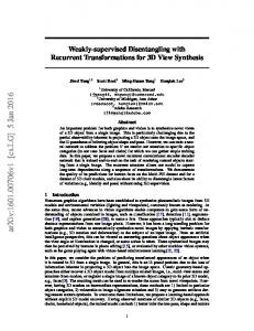
Abstract We propose a novel method for weakly supervised semantic segmentation. Training images are labeled only by the classes they contain, not by their location in the image. On test images instead, the method predicts a class label for every pixel. Our main innovation is a multi-image model (MIM) - a graphical model for recovering the pixel labels of the training images. The model connects superpixels from all training images in a data-driven fashion, based on their appearance similarity. For generalizing to new test images we integrate them into MIM using a learned multiple kernel metric, instead of learning conventional classifiers on the recovered pixel labels. We also introduce an “objectness” potential, that helps separating objects (e.g. car, dog, human) from background classes (e.g. grass, sky, road). In experiments on the MSRC 21 dataset and the LabelMe subset of [18], our technique outperforms previous weakly supervised methods and achieves accuracy comparable with fully supervised methods.

road dog

road cat

water boat

water boat

car tree road

car tree road buildings

water buildings sky

dog tree body face

Semantic segmentation on test set

Figure 1: Given a training set of images labeled only by the classes they contain (top), we learn a classifier that segments and recognizes visual classes in new test images (bottom).

beled. A few works have addressed the weakly supervised setting [25, 24], but none achieved performance comparable to fully supervised methods. A more detailed overview of related work is given in sec. 5. In this paper we present a weakly supervised method that, for the first time, achieves results competitive with fully supervised methods. Our main innovation is the multiimage model (MIM) - a graphical model that integrates observed image features and image labels together with latent superpixel labels over the whole training set into one network. We use MIM to jointly estimate the parameters of local appearance models for the semantic classes and to infer latent superpixel labels. For segmenting test images, we integrate them into MIM by means of a learned multiple kernel image similarity. As a secondary contribution, we introduce an “objectness” potential based on [2], which facilitates separating between object classes (e.g. cars, dogs, tables) from background classes (e.g. grass, road, water). As demonstrated on the MSRC 21 and the LabelMe subset of [18], the combination of these innovations enables to improve over the state-of-the-art in weakly supervised semantic segmentation performance, reaching a level comparable with fully supervised methods (sec. 6).

1. Introduction In this paper we consider the problem of semantic segmentation, where one has to predict a label for every pixel in the image. Labels correspond to semantic classes such as cars, dogs and trees. We are interested in learning a classifier for this task from weakly supervised data: each training image is annotated by labels specifying which classes are present in the image, but no pixel-level annotation is given (Fig. 1). This problem is very challenging because the method has to recover latent pixel labels from just presence labels, before it can generalize from the training set to test images. Recently there has been significant progress in fully supervised semantic segmentation [15, 14, 12, 21, 22, 26], although the problem is still unsolved. The disadvantage of fully supervised techniques is the need for manually labeling pixels in the training set, which is time consuming and expensive. Performance of such systems is inherently limited, since only small training sets can be manually la1

Algorithm 1 MIM construction at training time Input: sets of image superpixels and image labels τ =   oN n 0 Nj , distance function D xji , xji0 → R, ,Y j {xji }i=1 j=1   0 parameters k, p. Let ρ xji , xji0 be the distance between the center of mass of two superpixels, normalized by image dimensions. Output: multi-image connection set M .

Y3 A,C

Y4 D,F,G

X4

X3 X2

Y2 A,B

X5

X1

1. initialize: M = ∅

Y5 G,E

Y1 B,C

2. for each superpixel xji in each image I j  0  0 0 Nj (a) for each image I j = {xji }i=1 , Y j with T 0 Y j Y j 6= ∅ 0

N

j j do among  all superpixels {xi0 }i0 =1 with 0 ρ xji , xij0 < 0.3, select the p most similar 0

0

0

superpixels Bxj j = {xjl }pl=1 according to D i

0

(b) construct Bxj = ∪j 0 Bxj j i

i

(c) keep in Bxj only the k most similar superpixels i   0 0 (d) add connection yij , yij0 to M for all xji0 ∈ Bxj i

3. Return M

Figure 2: MIM at training time, for five images and full label set Y = {A,B,C,D,E,F,G}. Blank nodes represent latent superpixel  labels yij . They are connected to observed superpixel features  j xi and image labels Y j . Superpixels are interconnected by two sets of connections S and M . S connects spatial neighbors in individual images and M connects superpixels between images sharing a label.

We first describe MIM on an abstract level and provide implementation details in sec. 4. Fig. 2 shows a graphical representation of MIM. The total energy E of MIM is a function of latent superpixel labels yij and local appearance model parameters θ:   E {yij }, θ =

X

    ψ yij , xji , θ + π(yij , Yij ) +

xji ∈I j ;I j ∈τ

  0 0 φ yij , yij0 , xji , xji0 +

X

2. Multi-Image Model (MIM)

0

The backbone of our approach is MIM - a graphical model of a set of weakly labeled training images. MIM is based on a network of superpixels from all training images. The connections between superpixels capture their appearance similarity and spatial relations. In this section we address the problem of recovering the latent labels of superpixels in the training set, by finding the approximate MAP state of MIM. In sec. 3 we extend MIM for labeling superpixels on novel test image, for which no annotation at all is given. Images are represented as sets of superpixels, obtained by the oversegmentation algorithm [17]. Let τ = n  oN Nj I j = {xji }i=1 ,Y j be the training set, where inj=1

stances xji correspond to superpixels, coming in bags I j corresponding to images. Each bag has a label set Y j , which is a subset of the full label set Y ={1, ..., C}, corresponding to classes (Y j ⊂ Y ={1, ..., C}). Every instance xji has an associated latent label yij ∈ Y j . The bag label set YSj contains the labels of all instances in that bag (Y j = yij ). The task of weakly supervised learning is to recover the latent labels yij and to learn a classifier that predicts labels for each superpixel in a new image.

  0 0 φ yij , yij0 , xji , xji0

X 0

(yij ,yij0 )∈S

(yij ,y ji0 )∈M

(1) 



is a unary potential ψ yij , xji , θ , meathe local appearance of xji matches la-

The first term

suring how well bel yij , according to a classifier parameterized by θ. If f (x, θ) → RC is a multiclass classifier (e.g. a Random Forest) outputting probabilities fy (x, θ) for superpixel x taking label y, then we can define the unary potential as ψ (y, x, θ) = − log fy (x, θ). Our particular choice of f is described in sec. 4. The second unary potential π(yij , Yij ) assumes ∞ on labels outside Y j and zero otherwise, making sure yij ∈ Y j . The pairwise potential φ encourages connected superpixels to take the same label if their appearance similarity is high:

φ



0 0 yij , yij0 , xji , xji0

where D



0 xji , xji0





( =

  0 0 1 − D xji , xji0 yij 6= yij0 0

0

yij = yij0

,

(2) is a similarity metric between two su-

perpixels, scaled to [0, 1]. Our particular choice of similar-

ity metric is discussed in sec.4.  Note0 how these potentials are submodular, since 1 − D xji , xji0 ≥ 0 always. The pairwise potential is defined over two separate sets of connections - M and S. The first set S connects adjacent superpixels in the same image, to encourage spatially smooth labelings, as in [22]. The second set M is built in a data-driven fashion, by connecting similarTsuperpixels 0 between different images sharing a label (Y j Y j 6= ∅). These multi-image connections are an important novel characteristic of MIM. Constructing multi-image connections. The natural representation of a single image is a graph, where each (super)pixel is connected to its spatial neighbors [22, 1]. We propose to transcend individual images and define a structure over the whole training set. Superpixels with similar appearance and position from images that share weak labels are connected. Ideally, we could connect all the superpixels between all images sharing labels, but this would produce a hardly manageable, overly complex model. The intuition is that connections between superpixels with high appearance similarity contribute most to the energy, since the pairwise potential for very dissimilar superpixels is close to zero. Therefore, we keep the size of the model manageable by connecting each superpixel to a total of only k most similar superpixels in other images, and to at most p superpixels in one image. Also, the position of superpixels is taken into account by connecting only pairs of superpixels whose position in their respective images is closer than 3/10 of the image size. This is done to facilitate separating classes with similar appearance but different positions (e.g. sky and water). Algorithm 1 provides details. Inference. Minimizing the energy in eq. (1) maximizes the probability of superpixel labels yij and appearance model parameters θ, given observed superpixel features xji and image labels Y j . Under fixed parameters θ the energy is submodular. Since it is a multilabel problem, we cannot obtain global minima, but we can efficiently find a good approximation using the Alpha Expansion algorithm [13, 3, 5, 4]. If the labeling {yij } is fixed, the parameters θ can be estimated using supervised learning methods. Therefore, we alternate between these two steps to efficiently determine both parameters θ and labeling {yij }. As an initialization for θ, a solution from previous weakly supervised methods [25] can be used. We provide details on estimating and initializing θ in sec. 4.

3. Generalizing to the test set Having recovered the latent labels yij over the training set τ and learned parameters θ, we want to segment a new test image I t = {xti } for which no label at all is given. An obvious way is to use the trained classifier ψ (y, x, θ) on the superpixels of I t , and possibly smooth out the labeling by

I1

I3 y i1

y i3

It y it

I4

I2 y i2

y i4

Figure 3: The MIM model at test time. The test image I t is integrated into MIM through its q = 4 nearest training images (according to similarity metric K). The latent test superpixel labels yit are connected to superpixel’s features X t = {xti }, adjacent labels and labels of training images superpixels yij . Note, that the training superpixel’s yij labels are observed (groups of 4 shaded nodes in the corners of the figure).

using the spatial pairwise potentials. Instead, we want to use the full potential of MIM and integrate the test image into it. Let {xti } be the test image superpixels and {yit } their associated latentlabels. We infer these labels by minimizing:
X


E {yit } = ψ yit , xti , θ∗ + µ yit , I t + i

X (yit ,yij0 )∈S


φ yit , yit0 , xti , xti0 +

X

  φ yit , yij0 , xti , xji0

(yit ,yij0 )∈M t

(3) This energy function is analog to that used for training in eq (1). The first term consists of the appearance potential ψ, with parameters θ learned during training. The second term µ (yit , I t ) is a new Image Level Prior (ILP) potential inspired by [21]. During MIM training, we modulated ψ with an π(yij , Yij ) forcing superpixels to take a label given to the image. Of course, this cannot be done for I t , as its labels Y t are unknown. In (3) its role is played by the ILP potential µ (yit , I t ), which estimates the probability that I t contains class yit . This estimator is based on global appearance features, computed over the whole image, and can be learned with supervised learning techniques, since image labels are available during training (details in subsec. 3.1). The pairwise potentials φ are defined over adjacent superpixels S in the test image, as during training. The multiimage connections M connect test image superpixels to superpixels of training images. Since the training superpixel labels yij are fixed, these pairwise potentials depend only on test superpixel labels yit during the optimization of (3), which effectively turns them into unary potentials. This makes optimization easier. To build multi-image connections from the test image to training images we use Algo-

Algorithm 2 Integrating a test image into MIM.  N t Input: training set τ = I j j=1 , test image I t = {xti }N i=1 ,   0 distance function between superpixels D xji , xji0 → R,
t j distance function between  images K I , I → R, parameters k, p, q. Let ρ xti , xjl be the distance between the center of mass of two superpixels, normalized by image dimensions. Output: connection set M t 1. select set N of the q training images most similar to
test image according to K I t , I j

pares images based on different global features (GIST, color and quantized SIFT histograms; see sec. 4 for details). The main difference to [9] is that we learn a different metric for each training image instead of a universal one. This imagespecific metric enables images to place different weights on the kernels. Thus an image with water or grass will rely more on color features, while images of faces or cars will prefer local feature descriptors. We experimentally found this approach to have higher accuracy of predicting image tags in our setting. Our similarity metric is defined as follows
X j
K I t, I j = wk Kk I t , I j

2. for each test superpixel xti

(4)

k

(a) for each training image I j ∈ N N

j do among all superpixels {xjl }l=1 with  j t ρ xi , xl < 0.3, select the p most similar

superpixels Bxj t = {xjl }pl=1 according to D

where wkj is the weight of the k th kernel for training image I j . We learn the weights on the training set by maximizing the likelihood of training labels, weighted by their frequency over the training set as in [9]. The likelihood of a label y to be present in the image label set Y i is

i

(b) construct Bxti = ∪j Bxj t ; i

(c) keep in Bxti only the k most similar superpixels   (d) add connection yit , ylj to M t for all xjl ∈ Bxti ; t

3. output M .

rithm 2. Now we do not have access to the test image labels, so we cannot easily choose a set of training image to connect it to. For this, to use a learned image  we 0propose  similarity metric K I j , I j → R to find the most similar training images to I t and connect it to MIM through them (see subsec. 3.1 for details on K). We first find the q most similar training images. We then connect superpixels {xti } from I t to k most similar superpixels in these training images, but to at most p superpixels per image. This process is described in Algorithm 2. Fig. 3 shows a graphical representation of MIM at test time. For optimization we use Alpha Expansion again and estimate the labels yit of the test image I t .

3.1. Learning image metrics and ILP The proposed scheme for labeling the test image I t involves a similarity metric K and the ILP potential µ. We explain here how to learn K and how to use it in the ILP to predict test image labels. We use a nearest neighbor approach inspired by [9], which predicts the labels of the test image based on the labels of the few most similar training images, according to K. We define several image kernels and learn K as their linear combination. Each kernel com-

P y∈Y

i




q

1 X exp −K I i , I j |1y∈Y j − |, (5) = Z j=1

where Z is a normalizer making sure that result is in the unit interval. Having separate weights for each training image only increases the number of parameters, but otherwise does not change the training problem. Therefore, we refer to [9] for the training algorithm. After learning, the metric K is used to build connections in Algorithm 2 and within the ILP potential, which is defined as µ (yit ) = − log P (yit ∈ Y t ), where P (yit ∈ Y t ) is computed according to eq. 5.

4. Image features and local appearance models We define here the local appearance model ψ and the superpixel similarity metric D used in MIM. Superpixel features and potentials. We use Semantic Texton Forests (STF) [21] in both unary and pairwise potentials. STF is a local per pixel random forest classifier which uses very simple and fast features, such as the color difference between two pixels. We train it from the weakly supervised training set τ , using the geometric context dataset [10] as an auxiliary task, as proposed in [25]. The per-pixel output of the STF is then averaged over the pixels in a superpixel xji to predict a score fy (xji , θ) for each class y. The two main parameters of STF are the structure of the trees (split rules in the nodes) and the class scores in the leaves. As shown in [25], the structure of the forest obtained by multitask learning on the geometric context dataset approximates well the structure of a forest learned from a fully supervised semantic segmentation dataset [21]. Thus, in this

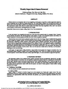
paper we keep the structure of the forest fixed and only estimate the class scores θ in the leaves from the weakly supervised segmentation dataset τ . To initialize θ, we use method of [25] on the same dataset τ . We globally rescale scores in the leaves to [0, 1] for each class over the whole training set, to ensure that infrequent classes are not overwhelmed by the frequent ones. To produce pairwise potentials φ, we use the Bags of Semantic Textons (BoST) representation produced by the STF [21]. BoST is a histogram concatenating the occurrences of tree nodes across the different trees when each pixel in a superpixel is passed through the STF. For every  pair of superj j0 pixels we can then define the similarity D xi , xi0 using a hierarchical histogram difference kernel, as in [21]. This metric D is used to define the pairwise potentials φ in eq. 2 and to connect superpixels between images in algorithms 1 and 2. We scale φ by median of maximum per superpixel contribution of all pairwise potentials to energy in MIM to make them comparable to unary potentials. Objectness potential. The classes to be segmented can be partitioned in two groups: objects such as bikes, animals and cars, and backgrounds, such as sky, grass and road. Objects have a well defined boundary and shape, as opposed to amorphous background regions. Background classes occupy most of the image and in weakly supervised case, they tend to “flood” areas belonging to objects [18], because of much higher frequency of background labels. To counter this effect, we use the objectness measure of [2], which estimates the probability that an image window contains an object of any class. Objectness combines several image cues measuring distinctive characteristics of objects, such as appearing different from their surroundings, having a closed boundary, and sometimes being unique within the image. We add to the unary potential of MIM a measure of the objectness of a superpixel. We start by sampling 104 windows using [2] according to their probability of containing an object 1 . Then we convert this measure to per-pixel probabilities by summing the objectness score over all windows covering a pixel, and globally normalizing the result over the whole training set. Finally, we convert the per-pixel probabilities to per-superpixel ones P (y ∈ Obj|x), by averaging over all pixels in a superpixel. The overall unary potential is defined as ψ (y, x, θ) = (

− log fy (x, θ) P (y ∈ Obj|x) y ∈ Obj − log fy (x, θ) (1 − P (y ∈ Obj|x)) y ∈ / Obj

(6) where Obj is the set of object classes. Note how the objectness potential for a superpixel we propose here is different 1 We used the source code released by the authors of [2] at http:// www.vision.ee.ethz.ch/˜calvin/software.html

x

w4 w w1 2

w3

3 Figure 4: Illustration of objectness. A pixel’s objectness is the average objectness over all window containing it. The normalization is global over the whole training set.

from the one in [6], which is directly the objectness probability for a window. Image kernels. For metric learning, we use three kernel types - GIST [20], color histograms and quantized SIFT [19] histograms (gray scale and color). GIST is computed over the whole image. Color and SIFT histograms are computed over the whole image and separately for three horizontal strips. SIFT histograms are also computed in spatial pyramids [16]. These spatial partitionings introduce some degree of localization in the global descriptors, making them more distinctive. To compute the distances from the descriptors we use L2 as the base metric for GIST, and χ2 for the rest.

5. Related work Semantic segmentation has attracted a lot of attention, but most works have focused on the fully supervised setting, where pixel labels are given for the training images [15, 14, 12, 21, 22, 26]. The basic approach was formulated in [22], where a conditional random field (CRF) was defined over image pixels with unary potentials learnt by a boosted decision tree classifier over texture-layout filters. The main research direction for successive publications focused on improving the CRF structure, enabling inference for multiple segmentations and introducing hierarchy with higher order potentials [14, 12, 8] and integrating label cooccurence statistics into it [15]. Another development were faster and more accurate features [21]. Towards less supervision, the extreme case is unsupervised object discovery, where unlabeled images of multiple classes are given [23]. Our weakly supervised setting is in the middle between the unsupervised and fully supervised cases (i.e. we only have image labels on the training set). To our knowledge, the same setting as ours was considered only in few previous works [25, 24, 7]. The earliest work [7] considered an image with a set of accompanying words. The authors posed the problem as machine translation and used an EM-type algorithm to solve it. In [24] a matrix factorization approach (pLSA) was proposed for estimating the per-pixel labels. In [25] a multiple instance and

Objectness

+

Original image

STF

Combined potential

Full MIM

+ ILP

Figure 5: Image illustrates the pipeline of the system on the test image - first unary potentials are produced by combining STF and objectness prior, then ILP reweights class’s scores according to global features and then result is passed onto MIM.

multitask learning modification of STF [21] was proposed. The STF structure was learnt in a multitask fashion with geometric layout estimation [10] as the auxiliary task. Multiple instance learning, specialized for semantic segmentation, was used to reconstruct the scores in the leaves of the STF. Because of the computational efficiency of the STF, we use the output of [25] to initialize the unary potentials of our MIM. However, the output of [24] could be used instead. The two weakly supervised previous works we compare to [25, 24] can be seen as special cases of our MIM model (trained in a different manner). The model [25] corresponds to omitting all connections between superpixels and training appearance models using multiple instance learning. The model [24] has connections, but only within individual images. In contrast, MIM forms a larger structure over the entire training set, connecting superpixels between images. This regularizes the training of appearance models and better recovers superpixel labels. Labeling a test image is also different from [25, 24] and most existing works. Instead of simply applying the learned appearance models, we connect the test image to the network of training images using learnt image similarities. Also related are single-class weakly supervised segmentation methods [1, 11]. They consider one class against background and typically show no test time scenario. Analog to our work, [1] also connects superpixels between images, but it does so in a predetermined fashion, encouraging superpixels at similar image positions to be either both foreground or both background. Instead, we connect in a data-driven fashion, factoring in also appearance similarity. Finally, our work is related to [6] by the use of an objectness potential. However, ours is defined on superpixels rather than windows [6]. Importantly, our task is different than that in [6]. While we consider learning a multi-class segmentation model, [6] learns a bounding-box object detector for a single class. As a consequence, our MIM model differs substantially from the one in [6]. For example, the nodes in MIM are image elements (superpixels) with class labels as states, whereas nodes in [6] are images with candidate windows as states.

6. Experimental results MSRC-21. We validate our method on the MSRC 21 dataset[22], containing 591 images of 320x213 pixels, accompanied by ground-truth segmentations of 21 classes We use standard split into training and test set as defined in [22]. This dataset is best suited for our task, as all classes are labeled in all images and there is significant co-occurrence between classes. Methods are typically compared using the total measure (percentage of correctly classified pixels) or the average per-class measure (percentage of correctly classified pixels for a class, averaged over all classes). The average criterion is preferable as it gives equal contribution to classes with large and small expected area in the images (e.g. dogs vs sky). We set the parameters for algorithms 1 and 2 as k = 21, p = 3, q = 5. For the objectness prior, classes sky, road, water, buildings and grass are considered to be background and the rest belongs to object classes. We use the objectness implementation released 2 by the authors of [2], whose parameters were estimated on a diverse set of 50 images randomly sampled from various datasets (see [2]). None of the images for training objectness come from the MSRC 21 dataset. Table 1 gives the results for our approach on this dataset. We compare to other semantic segmentation methods, both fully supervised (FS [22, 21, 14]) and weakly supervised (WS [24, 25]). Our method substantially outperforms both previous weakly supervised approaches. It achieves 17% better average per class accuracy than the next best method [24]. Interestingly, our method is even competitive with some fully supervised techniques, as it outperforms [22] and matches [21] (but it is below the recent state-of-the-art method [14]). We have also implemented a fully supervised version of our approach. In this case, the STF was trained fully supervised. There was no training stage for MIM, since the superpixel labels were known. Objectness, image similarity metric K and ILP were used in the same fashion as in weakly supervised scenario. At test time, labels of training superpixels in MIM were set to the ground-truth labels and test image was integrated using metric K. Experimenters show, that fully supervised version of our approach delivers 2 http://www.vision.ee.ethz.ch/

calvin/software.html

LabelMe [18]. To confirm our results on a second dataset, we performed additional experiments on the LabelMe subset of [18]. It contains 2500 images with 34 classes and it is more challenging than MSRC-21. As in MSRC-21, all classes are labeled in every image and there is significant co-occurrence between classes. All training parameters were kept the same as for MSRC-21. We obtain 14% average per-class accuracy with our weakly supervised method. This is better than the fully supervised TextonBoost [22] (13%) and worse than the fully supervised method of [18] (24%, see fig. 9 in [18]; do not confuse with per-pixel accuracy). To our knowledge, no weakly supervised results were reported on this dataset yet. Scalability. A modest computational complexity is important when considering scaling to thousands of images and hundreds of categories. When training our method, the largest cost is constructing the MIM. Complexity grows quadratically with the number of images per class, but linearly with the number of classes, since only images sharing a label are connected. Therefore, scaling to thousands of images distributed over many classes is possible. At test time, we first search for the k most similar images in the training set (linear time) and then connect only their superpixels to the test image (algo. 2). Most importantly, training superpixel labels are fixed, so inference is performed only on the superpixel labels of the test image (sec. 3). Inference for an image takes only 7 seconds on a 2.66 GHz 64-bit Intel processor.

7. Conclusion We presented a weakly supervised semantic segmentation method that, for the first time, can compete with fully supervised ones. Our main contribution is MIM - a graphical model for weakly supervised semantic segmentation with data-driven structure. MIM elegantly formalizes a simple intuition of weakly supervised learning - similar superpixels in images sharing a label are likely to belong to the same class. We have also introduced an objectness unary potential, that distinguishes objects from background classes. At test time, we integrated the test image into MIM by using multiple kernel metric learning.

total

average

total

train

average

test

objectness

Evaluation of components. We individually analyze the impact of using MIM (for both training and testing) and objectness on the average and total accuracy measures. As we can see in table 2, both proposed components contribute to accuracy. Note how MIM delivers most improvement on average accuracy when combined with the objectness potential, which protects smaller object regions from being flooded by background (e.g. a bird in the sky).

STF based ψ, φ on S and µ+ MIM

performance comparable to the state-of-the-art (last row of table 1). While using simpler features and no higher order potentials, it is just 3% below [14].

-

-

53

46

51

63

yes

-

55

58

66

70

-

yes

59

56

77

70

yes

yes

67

67

83

80

Table 2:

Evaluation of our proposed novel components on MSRC21. We test our technique with different components active on top of the basic weakly supervised STF with ILP and pairwise potentials only on S (top row). The two components are: inference on the full MIM (both on training and test set) and using the objectness potential. We measured total per pixel accuracy and average per class accuracy.

Future work will focus on far larger training sets, which we believe will highlight the advantage of our approach vs fully supervised ones. In principle, MIM can easily integrate different levels of supervision, which might be another interesting direction of research. We also plan to extend MIM to higher order potentials as in [14]. Acknowledgements A. Vezhnevets was supported by the SNSF under grant #200021-117946. V. Ferrari was supported by a SNSF Professorship.

References [1] B. Alexe, T. Deselaers, and V. Ferrari. Classcut for unsupervised class segmentation. In ECCV, 2010. [2] B. Alexe, T. Deselaers, and V. Ferrari. What is an object? In CVPR, 2010. [3] Y. Boykov and M.-P. Jolly. Cuts for optimal boundary and region segmentation of objects in n-d images. In CVPR, 2001. [4] Y. Boykov and V. Kolmogorov. An experimental comparison of mincut/max-flow algorithms for energy minimization in vision. TPAMI, 2004. [5] Y. Boykov, O. Veksler, and R. Zabih. Efficient approximate energy minimization via graph cuts. TPAMI, 2001. [6] T. Deselaers, B. Alexe, and V. Ferrari. Localizing objects while learning their appearance. In ECCV, 2010. [7] P. Duygulu, K. Barnard, N. de Freitas, and D. Forsyth. Object recognition as machine translation: Learning a lexicon for a fixed image vocabulary. In ECCV, 2002. [8] J. M. Gonfaus, X. Boix, J. V. de Weijer, A. D. Bagdanov, J. Serrat, and J. Gonzlez. Harmony potentials for joint classification and segmentation. In CVPR, 2010. [9] M. Guillaumin, T. Mensink, J. Verbeek, and C. Schmid. Tagprop: Discriminative metric learning in nearest neighbor models for image auto-annotation. In ICCV, pages 309–316, sep 2009. [10] D. Hoiem, a.a. Efros, and M. Hebert. Geometric context from a single image. In ICCV, 2005. [11] W. J. and J. N. Locus: learning object classes with unsupervised segmentation. In ICCV, 2005. [12] P. Kohli, L. Ladicky, and P. Torr. Robust higher order potentials for enforcing label consistency. In CVPR, 2008. [13] V. Kolmogorov and R. Zabih. What energy functions can be minimized via graph cuts? In ECCV, 2002. [14] L. Ladicky, C. Russell, and P. Kohli. Associative hierarchical crfs for object class image segmentation. In CVPR, 2009.

building

grass

tree

cow

sheep

sky

airplane

water

face

car

bicycle

flower

sign

bird

book

chair

road

cat

dog

body

58

62

98

86

58

50

83

60

53

74

63

75

63

35

19

92

15

86

54

19

62

7

[21], FS

67

49

88

79

97

97

78

82

54

87

74

72

74

36

24

93

51

78

75

35

66

18

[14], FS

75

80

96

86

74

87

99

74

87

86

87

82

97

95

30

86

31

95

51

69

66

9

[25],WS

37

7

96

18

32

6

99

0

46

97

54

74

54

14

9

82

1

28

47

5

0

0

boat

average [22], FS

[24],WS

50

45

64

71

75

74

86

81

47

1

73

55

88

6

6

63

18

80

27

26

55

8

Ours, WS

67

12

83

70

81

93

84

91

55

97

87

92

82

69

51

61

59

66

53

44

9

58

Ours, FS

72

21

93

77

86

93

96

92

61

79

89

89

89

68

50

74

54

76

68

47

49

55

Table 1: MSRC 21 results. Our method compared to the state-of-the-art in semantic segmentation. WS denotes weak supervision, FS full

Result of MIM Unary potentials Original image

Result of MIM Unary potentials Original image

supervision. Our WS approach outperforms any existing WS technique and is even competitive with some of the FS ones. In bold, classes on which our WS algorithm performs better than other methods. Note, how we are able to recognize two very hard classes (boat and bird) substantially better than any previous methods (either weakly or fully supervised). The modest result of our method on the body class in the WS case can be explained by the high co-occurrence of face and body labels in the training set.

Figure 6: Segmentations on the MSRC test set. Row 1,4: Original images with overlayed ground truth. Row 2,5: output of unary potentials (only the label with maximum score is shown). Row 3,6: results of the full system with MIM. Note how the inference with integration of test image into MIM significantly improves results on images with many classes. [15] L. Ladicky, C. Russell, P. Kohli, and P. Torr. Graph cut based inference with co-occurrence statistics. In ECCV, 2010. [16] S. Lazebnik, C. Schmid, , and J. Ponce. Beyond bags of features: Spatial pyramid matching for recognizing natural scene categories. In CVPR, 2006. [17] A. Levinshtein, A. Stere, K. N. Kutulakos, D. J. Fleet, S. J. Dickinson, and K. Siddiqi. Turbopixels: Fast superpixels using geometric flows. TPAMI, 31:2290–2297, 2009. [18] C. Liu, J. Yuen, and A. Torralba. Nonparametric scene parsing: label transfer via dense scene alignment. In CVPR, 2009. [19] D. G. Lowe. Object recognition from local scale-invariant features. In ICCV, 1999. [20] A. Oliva and A. Torralba. Modeling the shape of the scene: A holistic representation of the spatial envelope. International Journal of Computer Vision, 42:145–175, 2001.

[21] J. Shotton, M. Johnson, and R. Cipolla. Semantic texton forests for image categorization and segmentation. In ECCV, 2008. [22] J. Shotton, J. Winn, C. Rother, and A. Criminisi. Textonboost: Joint appearance, shape and context modeling for multi-class object recognition and segmentation. In ECCV, 2006. [23] T. Tuytelaars, C. H. Lampert, M. B. Blaschko, and W. Buntine. Unsupervised object discovery: A comparison. IJCV, 88(2), 2010. [24] J. Verbeek and B. Triggs. Region classification with markov field aspect models. In CVPR, 2007. [25] A. Vezhnevets and J. Buhmann. Towards weakly supervised semantic segmentation by means of multiple instance and multitask learning. In CVPR, 2010. [26] L. Yang, P. Meer, and D. J. Foran. Multiple class segmentation using a unified framework over mean-shift patches. In CVPR, 2007.